HAL Id: hal-00316235
https://hal.archives-ouvertes.fr/hal-00316235
Submitted on 1 Jan 1996
HAL is a multi-disciplinary open access
archive for the deposit and dissemination of sci-entific research documents, whether they are pub-lished or not. The documents may come from teaching and research institutions in France or abroad, or from public or private research centers.
L’archive ouverte pluridisciplinaire HAL, est destinée au dépôt et à la diffusion de documents scientifiques de niveau recherche, publiés ou non, émanant des établissements d’enseignement et de recherche français ou étrangers, des laboratoires publics ou privés.
On the seasonal effect of orbital variations on the
climates of the next 4000 years
Julián Adem
To cite this version:
Julián Adem. On the seasonal effect of orbital variations on the climates of the next 4000 years. Annales Geophysicae, European Geosciences Union, 1996, 14 (11), pp.1198-1206. �hal-00316235�
Ann. Geophysicae 14, 1198—1206 (1996) ( EGS — Springer-Verlag 1996
On the seasonal effect of orbital variations on the climates
of the next 4000 years
Julia{ n Adem
El Colegio Nacional and Centro de Ciencias de la Atmo´sfera, UNAM, 04510, Me´xico, D. F., Me´xico
Received: 10 March 1995/Revised: 20 March 1996/Accepted: 17 April 1996
Abstract. A northern hemisphere thermodynamic climate model is used to compute the effect of the insolation anomalies due to orbital variations in the climates for the next 4000 years. Berger’s mean monthly anomalies of insolation are used in the computations, which are carried out for 1000, 2000, 3000 and 4000 years after present (kyears AP). The numerical simulations show that in the climates of the next 4000 years, due to the effect of the orbital variations, springs and summers will be increasing-ly dryer and falls and winters wetter than the present climate.
1 Introduction
In a previous study (Adem, 1989), using Berger’s (1978) insolation anomalies, the effect of the orbital variations on the climates from 4000 years ago to present was investi-gated. The results show important seasonal anomalies of temperature and precipitation, despite the fact that for that period the annual average of the insolation anomalies was negligibly small. Similarly in this study I use Berger’s (1978) insolation anomalies for the next 4000 years to explore the effect of the orbital variations on future cli-mates during this period.
2 The model
The model used is the version of the thermodynamic model described in detail in previous papers (Adem, 1982, 1991). It consists of an atmospheric layer 10 km high which includes a cloud layer, an oceanic layer 50 m in depth, and a continental layer of negligible depth. The model also includes a layer of snow and ice, whose hori-zontal extent is computed internally.
The basic predicting equation is the conservation of thermal energy which applied to the atmospheric layer
and to the oceanic (or continental) layer yields two equa-tions which contain as variables the mean atmospheric temperature (¹m), and the surface ocean and continental ground temperature (¹s), as well as the heating and trans-port terms.
The other conservation laws are used diagnostically, together with semi-empirical relations, to parametrize the heating and transport components. These parametriz-ations supply additional equparametriz-ations which, combined with the thermal energy equations, give rise to a system of simultaneous equations. This is solved with an implicit integration method, yielding, besides the temperatures, the heating functions and the anomalies of wind.
The parametrizations of the heating and transport terms are those described by Adem (1982), except for the modifications used by Adem and Gardun8 o (1984) in order to incorporate the conservation of water vapor in the model. The equations and the variables are averaged over a month, so that the horizontal transport of heat in the atmosphere by transient eddies is parametrized using a horizontal exchange coefficient equal to 3]106 m2 s~1 The snow-ice boundary is determined as a variable by assuming that it coincides with the 0 °C computed surface isotherm. This is accomplished by an adjusting process between surface albedo and surface temperature by which at each grid point an albedo for snow-ice cover is assigned when the computed surface temperature is lower or equal to 0 °C. An albedo for no snow-ice on the ground is assigned when the surface temperature is larger than 0 °C, as is described by Adem (1981a). The adjusting process converges rapidly due to the snow-ice temperature feed-back.
Starting in August, when the snow—ice cover is mini-mal, the model is iterated month by month until the dif-ference between the computed anomaly of the surface temperature, each month of the last year and the same month of the previous year of the run is smaller or equal to 0.01 °C.
In the version of the model used here, the precipitation anomalies are computed externally to the model, using
a multiple regression equation by Clapp et al. (1965), in which the anomaly of precipitation depends on three terms which are the anomaly of the mid-tropospheric temperature and its derivatives in the x and y directions, where x and y are the horizontal coordinates in the polar stereographic projection used in the model. The coeffi-cients of the three terms were obtained by a multiple regression procedure and are functions of the geographic position and the season, as described in the Appendix. Therefore the precipitation anomalies do not necessarily follow a pattern similar to the temperature anomalies. Furthermore, the formula corresponds to anomalies of the present climate with respect to the normal present values, and we are applying it to compute anomalies or depar-tures of the climates of the next 4000 years with respect to the normal present climate.
The model is hemispheric, the equations are monthly averaged, and the time step is of one month. The solution is obtained after about 6 years of integration, and is presented as a set of monthly charts for the surface ocean and continental ground temperature, the mid-tropo-spheric temperature, the precipitation, and the heating and transport terms.
The equations of the model are solved first using the present insolation to simulate the present climate, and then using as forcing function the insolation computed by Berger (1978) for 1, 2, 3 and 4 kyears AP to simulate the corresponding climates. Subtracting the computed pre-sent values from the computed values for each of these periods, the corresponding anomalies are obtained.
It is assumed that for these cases the permanent ice sheet is the same as at present, however, a month-to-month variable snow-ice extent is computed, whose boundary is determined by the 0 °C computed surface ocean and continental ground isotherm, in the way de-scribed already. Water vapor and clouds feedbacks are not included in the version of the model used in these simulations.
The simulation of the present climate will not be shown here because it has been given in previous studies (Adem, 1982, 1991). The results show that the model simulates reasonably well the annual cycle of the present climate, including the snow-ice boundary. Furthermore the simu-lation of the climate for 18 kyears BP has shown that the computed anomalies of surface ocean and continental ground temperature are in relatively good agreement with the values computed for the oceans by CLIMAP (1981) and for the continents with the values published by Gates (1976a) which are based on analysis of fossil pollen and other periglacial evidence from several available sources (Adem, 1981a, b)
The northern hemisphere average continental ground temperature for July of 18 kyears BP, has been compared with the value obtained by Gates (1976b) using a general circulation model, showing very good agreement.
The northern hemisphere average continental ground temperature computed by the model for July and January for 4 kyears BP shows good agreement with the corre-sponding surface air temperature value obtained by linear interpolation from Kutzback and Guetter (1986) numer-ical experiments for 6 and 3 kyears BP.
A general discussion of the overall performance of the model has been given in a previous study (Adem, 1991). Here I have mentioned only some of the results related to the simulation of the present and past climates to support the credibility of the results on the simulation of the future climates that I undertake in this work.
3 Simulation for 4 kyears AP
Figure 1 shows the northern hemisphere (NH) monthly mean insolation anomalies (departures from present values) as given by Berger (1978) for 4 kyears AP. In this figure, the ordinate is the latitude in degrees and the abscissa is the time of the year in months. The figure shows the isolines of the insolation anomalies with respect to present values in W m~2. This figure shows that the anomalies of insolation have a strong seasonal variation and a relatively small variation with respect to latitude. The anomalies for all latitudes are positive for spring and early summer and negative for late summer and fall; in winter they are relatively small.
Although the model computes maps for the 12 months of the year, Fig. 2 only shows the maps of the computed surface ocean and continental ground temperature anomalies for May (Fig. 2a) and October (Fig. 2b), which are the months when the NH averages of the computed anomalies have the largest absolute values. This figure shows that anomalies of a magnitude as large as several degrees Celsius, appear in large areas of the continents for both months, and the difference between them are in some regions as large as 4—5 °C from May to October. Over the oceans the anomalies are much smaller than in the continents.
Similarly Fig. 3 shows the precipitation anomalies for June and November, which are the months when NH averages of the computed precipitation anomalies have
Fig. 1. The mean monthly insolation anomalies in W m~2 for 4 kyears AP, after Berger (1978)
Fig. 2a, b. Ocean surface and continental ground temperature anomalies resulting from orbital variations isotherms in 0.1 °C for 4 kyears AP. a for May, b for October
Fig. 3a, b. Precipitation anomalies resulting from orbital variations, in mm per month, for 4 kyears AP; a is for June, b for November J. Adem: On the seasonal effect of orbital variations on the climates of the next 4000 years 1201
Fig. 4. a Zonally averaged continental ground temperature anomalies and b sea surface temperature anomalies resulting from orbital variations for 4 kyears AP (isotherms in 0.1 °C)
the largest absolute values. Important anomalies appear also in these cases, especially in lower latitudes.
In Fig. 4 are shown the zonally averaged values of the continental ground temperature anomalies (Fig. 4a), and of the ocean surface temperature anomalies (Fig. 4b). Continental ground temperature values are much larger than those of ocean surface temperature. Comparison of Fig. 4a with Fig. 1 shows that the continental ground temperature values are highly correlated with the values of insolation anomalies, having positive anomalies for spring and early summer and negative for late summer and fall. Furthermore, in winter the continental ground temperature anomalies are also relatively small. The lar-gest positive continental ground temperature anomalies are in lower and higher latitudes in May, with values of about 3 °C, and the largest negative anomalies occur in August at a latitude of 70°N, and are of about !3.0 °C.
Fig. 5. Zonally averaged precipitation anomalies due to orbital variations for 4 kyears AP (isotherms in 0.1 °C)
Figure 4b shows that the computed surface ocean tem-perature anomalies for 4 kyears AP are, except for sum-mer, of a magnitude not larger than 0.2 °C, negative in fall, winter and early spring, and positive in late spring and summer. In the summer there are anomalies as large as 0.9 °C in higher latitudes and 0.5 °C in lower latitudes.
The zonally averaged precipitation anomalies in the continental areas are shown in Fig. 5 where the abscissa is the time in months, the ordinate is the latitude in degrees, and the isolines are in mm per month. This figure shows that there is a strong negative precipitation anomaly that includes spring and summer, especially in lower latitudes, with values as large as 20 mm per month in June, and a positive anomaly in fall, with values as large as 15 mm per month also in the lower latitudes.
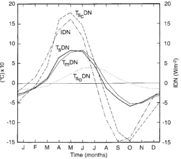
Figure 6 shows the NH averages of the ocean surface and continental ground temperature, the mean tropo-spheric temperature, and the insolation anomalies, due to the orbital variation for 4 kyears AP. The abscisa is the time of the year, in months, the ordinate on the left corresponds to surface temperature anomalies and is in 0.1 °C, and that on the right is the insolation anomalies in W m~2.
The thick continuous curve corresponds to the average value when all ocean surface and continental ground temperature anomalies are included, which will be de-noted by ¹sDN. The dashed and dotted curves corres-pond to the average values of the continental ground temperature anomalies and to the ocean surface temper-ature anomalies, separately denoted ¹scDN and ¹soDN
respectively. The dashed-dotted and thin continuous curves are the averages over the integration region (NH) of the mean tropospheric temperature and the insolation anomalies, denoted for brevity ¹mDN and IDN respec-tively.
For the case of 4 kyears AP, as shown in Fig. 6, the insolation anomalies (IDN) have positive values for the
Fig. 6. Average over the total integration region of the ocean surface and continental ground temperature anomalies together (thick
con-tinuous line), the continental ground temperature anomalies (dashed lines), the ocean surface temperature anomalies (dotted line), the
mean tropospheric temperature anomalies (thin continuous line), and the insolation anomalies (dashed-dotted line) for 4 kyears AP. The
ordinate to the left is for temperature anomalies in 0.1 °C and to the right is for insolation anomalies in W m~2
6 months from February to July, and negative for the other six months of the year, with the maximum in May and the minimum in September. The simulated sea surface temperature anomalies (¹soDN) are positive from April to
September, zero in October and negative for the rest of the year, with the maximum in July and the minimum in December-January.
Ocean effects
Comparison of ¹soDN with IDN in Fig. 6 shows that
the primary forcing function (IDN) has induced anomalies of sea surface temperature, which due to the storage of heat of the oceans have a lag of 2 months, and become a source of energy that affects the other climate variables. Figure 6 shows that due to the ocean effect the tropos-pheric temperature anomaly, ¹mDN, has a lag with re-spect to IDN of about a month, and the continental ground temperature has a lag of about two thirds of a month.
Comparison of ¹mDN with ¹sDN shows that the NH tropospheric temperature anomaly is of about the same magnitude as the average of the ocean sur-face and continental ground temperature together, having a lag of about one third of a month with re-spect to the same average. However, Fig. 7 shows that the magnitude of the tropospheric temperature anomalies is larger over the continents and smaller over the oceans than that of the surface temperature anomalies. As men-tioned before both anomalies are larger over the conti-nents than the oceans.
Fig. 7. Average over continents (thin dashed line) and over oceans (thin dotted line) of the mean tropospheric temperature anomalies; and average anomalies of continental ground temperature (thick
dashed line) and ocean surface temperature (thick dotted line)
These results show that the astronomical forcing for 4 kyears AP produces insolation anomalies computed by Berger (1978) which yield significant temperature anom-alies in the atmosphere-ocean-continent system.
Due to the storage of heat in the oceans the tem-perature anomalies have a lag compared to insolation anomalies, of about 2 months over the surface of the oceans, of about a month in the troposphere and of about two thirds of a month over the surface of the continents.
Due to the heat capacity of the ocean, and to the fact that the insolation anomalies are positive for the 6 months from February to July, and negative for the rest of the year, the ocean temperature anomalies are smaller than those over the continents. However, they become an inter-nal forcing factor that affect the tropospheric and conti-nental ground temperature as described already.
Albedo feedback
On average the albedo feedback is negligible. It is zero for December, January, February, March, June and July. However it is important in the other months at some localities due to anomalies of the snow-ice boundary, especially in spring in middle latitudes, causing an in-crease of temperature due to a more rapid melting of the snow than at present. In the late summer and early fall it causes a decrease of temperature at higher latitudes due to an excess of snow-ice condition compared to present con-ditions. These feedback effects are shown in Fig. 4a, as a positive maximum of 2 °C in middle latitudes in April, and a negative maximum of 3 °C in higher latitudes in August.
Fig. 8. Average values of continental ground temperature anomalies due to orbital variations, from present to 4 kyears AP (0.1 °C)
4 The evolution of temperature and precipitation anomalies from present to 4 kyears AP
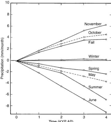
In a previous study (Adem, 1989), it has been shown that from 4 kyears BP to present the temperature deviations from today’s values decrease quasi-linearly. Something similar occurs for the deviations from present to 4 kyears AP. Simulation of the climates for 1, 2 and 3 kyears AP were also carried out. The computed maps of surface ocean and continental ground temperature, mean tropo-spheric temperature and precipitation anomalies show similar patterns to those for 4 kyears AP, with magnitudes reduced to about one quarter, one half and three quarters, respectively. Therefore the anomalies have the same sign and their magnitude shows a quasi-linear increase from present to 4 kyears AP, as shown in Figs. 8 and 9, where the average values in the NH of the continental ground temperature and precipitation anomalies are plotted re-spectively. In these figures the abscissa is the time in kyears AP, and the ordinate the mean continental ground temperature in tenths of degrees C and the mean precipi-tation anomaly in millimeters per month, respectively. The curves plotted in the figures have been constructed using the values of the simulations for 4, 3, 2 and 1 kyears AP, and show the evolution of the anomalies from present to 4 kyears AP.
5 Final remarks and conclusions
A NH thermodynamic climate model is used to compute the effect of the insolation anomalies due to orbital vari-ations in the climates for the next 4000 years. Berger’s mean monthly anomalies of insolation are used in the
Fig. 9. Average values of the precipitation anomalies due to orbital variations from present to 4 kyears AP, in mm per month
computations, which were carried out for 1000, 2000, 3000 and 4000 years after present (kyears AP). It is shown that due to the orbital variations for 4 kyears AP the climate will be warmer from March to July and colder from August to February than present. The temperature anomalies are much larger for the continents than for the oceans. For 4 kyears AP the averages of the continental ground temperature anomalies are !0.3, 1.3, 0.6 and !1.2 °C for winter, spring, summer and fall respectively. The geographic monthly distribution of these anomalies shows that they increase towards the lower latitudes with the largest positive values of about 2.0 to 3.0 °C from April to July, and the largest negative values of about 2.0 to 2.5 °C from October to November, below 20° latitude, for continental areas.
For 1, 2 and 3 kyears AP the computed surface temper-ature anomalies have a similar distribution to those for 4 kyears AP with a magnitude that increases quasilinearly from present to 4 kyears AP.
The numerical simulation shows that in the climates of the next 4000 years, due to the effect of the orbital vari-ations, springs and summers will be increasingly dryer and falls and winters wetter than the present climate.
In the numerical simulations the greenhouse gases are kept fixed, and equal to their present level, and the only forcing are the orbital variations. The results show that for the period from present to 4 kyears AP, due to the orbital variations, the average annual increase of temperature in the NH is !0.02, !0.01, 0.02 and 0.04 °C for 1, 2, 3 and 4 kyears AP, respectively, values which are negligibly small. Loutre (1995) using the two-dimensional climate model developed by Galle´e et al. (1991, 1992) in Louvain-la-Neuve, computed in a similar experiment an increase of
less than 0.2 °C of amplitude for the period from present to 5 kyears AP. Furthermore, from the results of Berger (1994), Kim et al. (1994), and Loutre (1995) it follows that for annual averages the climates from present to 4 kyears AP will be mainly affected by an increase of the greenhouse gases, and by vulcanism. The orbital vari-ations will play an important role only for longer time periods.
The purpose of this study is to show that for the near-future climates from present to 4 kyears AP the monthly and seasonal effects due to the orbital variation alone can produce significant changes in the annual cycle of these climates, despite the fact that the annual values are insignificant.
Acknowledgements. I am indebted to Jorge Zintzu´n for the
com-putational technical support, to Ma. Esther Grijalva and Thelma del Cid for their help in the preparation of the manuscript, and to Rodolfo Meza for his help in the preparation of the figures.
The Editor-in-Chief thanks T. Ledlleg and another referee for their help in evaluating this paper
Appendix A
¹he parametrization of the precipitation anomalies
To understand the limitations and the potential of the formula used for the precipitation computations it is necessary to go back to its original source. Its development is due to Clapp et al. (1965) who described the procedure to obtain the coefficients as follows: ‘‘(. . .) it has been found from extensive empirical-statistical studies (Smith, 1942; Stidd, 1954; Klein, 1963) that in specifying rainfall from mean circulation parameters (a requirement in the present case) it is better to employ statistical methods, using as independent variables easily-measured features of the large-scale circulation itself. In the present study, it was assumed that the anomaly of total monthly precipita-tion can be expressed as a simple linear funcprecipita-tion of the local anomalies of mean monthly temperature and west-east and south-north wind components at 700-mb. These three variables were chosen simply because the physical reasons for expecting them to be related to precipitation are well known, as will be clarified in the subsequent discussion. The following linear regression equation relates these variables:
R!RN"b(¹!¹N)#c(º!ºN)#d(»!»N), (1APP) where R is total monthly precipitation (inches); ¹, monthly mean temperature at 700 mb (K); and º and » the west-east and south-north wind components at 700 mb (m s~1, considered positive when from the west and south, respectively). The subscript N refers to normal or long-period averages, which in this study are the sample means.
The regression coefficients b, c and d were determined using approximately 12 years of monthly mean data (ending in March 1963) for 37 land or island stations scattered over the northern hemisphere. Data for individual stations were extracted from a va-riety of sources including WMO CLIMAT reports (US Weather Bureau II, 1963) and published climatological bulletins for indi-vidual countries. Wherever possible, monthly average temperatures and winds from upper-air (RAWIN) sounding were used, but where these were not available, temperatures and geostrophic winds were interpolated from manuscript maps of the Extended Forecast Divi-sion, US Weather Bureau.’’
‘‘(. . .) In spite of the inadequate data coverage and low correla-tions, an attempt was made to analyze the fields of the three coeffi-cients for each season. In attempting the analysis in the vast areas where there is no measured precipitation (mainly oceans) or where no computations were made, certain reasonable guidelines were
followed based on the available calculations and on synoptic experi-ence. Thus, it was concluded that the geographical pattern of the temperature coefficient (b) depends mainly on climate. Over central and northern continents in winter, precipitation tends to occur with above normal temperature, a relationship also true of high latitudes at all seasons and western oceans in summer and fall; and with below normal temperature over continents in summer, and at lower lati-tudes, along west coasts and over desert regions at all seasons. These associations are due partly to the influence of cloudiness on long-and short-wave radiation.
The distribution of the coefficients of the wind components was assumed to depend mainly on terrain and latitude. For example, where a westerly or southerly wind is directed from water to land, and especially if it is forced to ascend mountains, a strong positive relationship between rainfall and wind speed is found (west coasts of both continents). When directed downslope, these components are negatively related to rainfall. The south-north wind component tends to be positively related to rainfall almost everywhere due to the observed fact that convergence and rising motion prevails with south and the opposite with north winds (Panofsky, 1951). An interesting exception is the consistently negative coefficient at Bodo, Norway where the principal moisture source lies north of an east-west mountain chain. It was assumed that over southern oceans, at all seasons, heavy rains occur with easterly winds in conformity with observed rainfall in easterly waves and tropical storms.’’
‘‘(. . .) It is necessary to modify the regression equations for use in the model, because the latter predicts the mean temperature in mid-troposphere (approximately at 500-mb) and not the winds.
The mid-tropospheric temperature anomalies can be used dir-ectly in the first term on the right of equation 1APP, because there is probably little difference in the anomaly of monthly mean temper-ature at 500 and 700 mb. However, the two terms involving the winds must be transformed in two important respects. First, the predictions are made for a rectangular grid array of 512 points on a polar-stereographic projection whose X-axis points along the 10° E meridian and ½-axis along the 80°W meridian (Adem, 1964). Therefore, we must transform the eastward (º) and northward (») directed wind components to corresponding components º@ and »@; directed along the positive X- and ½- axes respectively. This involves a simple transformation of coordinates. The second transformation is to convert wind speed to a thermal wind (a measure of vertical wind shear), so that the wind components at 700 mb can be replaced by temperature gradients in mid-troposphere. This latter conversion is accomplished using approximations which are probably reason-ably valid for use with monthly mean charts; i.e., use is made of the well-known thermal-wind equations, together with the properties of the equivalent barotropic atmosphere (Charney, 1949), in which isotherms and isobars are parallel. The details of these transforma-tions will not be documented here.’’
The formula has been applied in monthly predictions of precipi-tation anomalies of the present climate with some success (Adem and Donn, 1981; Adem et al., 1995). The application of the formula for the next 4000 years is based on the assumption that it is valid for such a period relatively close to the present, and in which there are relatively small temperature and precipitation anomalies with re-spect to the present normal values. At present, research is being carried out to possibly improve the formula.
It is evident that the approach is realistic. However, con-siderable improvement in the results could be obtained by updat-ing the coefficients in the formula by the use of the much more complete data that is available at present. Furthermore, a similar formula has been developed by Oda-Noda (1995), which seems to improve the results, and that will be used in future numerical experiments
References
Adem, J., On the physical basis for the numerical prediction of monthly and seasonal temperatures in the troposphere-ocean-continent system, Mon. ¼eather Rev., 92, 91—103, 1964. J. Adem: On the seasonal effect of orbital variations on the climates of the next 4000 years 1205
Adem, J., Numerical simulation of the annual cycle of climate during the ice ages, J. Geophys. Res., 86, 12015—12034, 1981a. Adem, J., Numerical experiments on the ice age climates, Clim.
Change, 3, 155—171, 1981b.
Adem, J., Simulation of the annual cycle of climate with a thermo-dynamic numerical model, Geofi&s. Int., 21, 229—247, 1982 Adem, J., On the effect of the orbital variation on the climates from
4 thousand years ago to present, Ann. Geophysicae, 7, 599—606, 1989.
Adem, J., Review of the development and applications of the Adem thermodynamic climate model, Clim. Dyn., 5, 146—160, 1991. Adem, J., and W. L. Donn, Progress in monthly climate forecasting
with a physical model, Bull. Am. Meteorol. Soc., 62, 1666—1675, 1981.
Adem, J., and R. Gardun8 o, Sensitivity studies on the climatic ef-fect of an increase of atmospheric CO2, Geofi&s. Int., 23, 17—35, 1984.
Adem, J., A. Ruiz, V. M. Mendoza, and R. Gardun8 o, Recent experi-ments on monthly weather prediction with the Adem thermo-dynamic climate model, with especial emphasis in Mexico,
At-mo& sfera, 8, 23—34, 1995.
Berger, A., Long-term variations of daily insolation and quaternary climate changes, J. Atmos. Sci., 35, 2362—2367, 1978.
Berger, A., The Earth’s past and future climates, EGS Newsl., 53, 1—8, 1994.
Clapp, P. F., S. H. Scolnick, R. E. Taubensee, and F. J. Winninghoff, Parameterization of certain atmospheric heat sources and sinks for use in a numerical model for monthly and seasonal forecast-ing, Internal Report, Extended Forecast Division (available on request to Climate Analysis Center, NWS/NOAA, Washington, D.C. 20233), 1965.
Charney, J. G., On a physical basis for numerical prediction of large-scale motions in the atmosphere, J. Meteorol., 6, 371-385, 1949.
CLIMAP Project Members, Seasonal reconstruction of the Earth’s surface at the last glacial maximum, Geological Society of Amer-ica, Map and Chart series, MC-36, 1—18, 1981.
Galle´e, H., J. P. Van Ypersele, T. Fichefet, C. Tricot, and A. Berger, Simulation of the last glacial cycle by a coupled sectorially-averaged climate ice-sheet model, I. The climate model. J.
Geo-phys. Res., 96, D7, 13139—13161, 1991.
Galle´e, H., J. P. Van Ypersele, T. Fichefet, C. Tricot, and A. Berger, Simulation of the last glacial cycle by a coupled sectorially-averaged climate ice-sheet model. II. Response to insolation and CO2 variations, J. Geophys. Res., 97, D14, 15713—15740, 1992. Gates, W. L., Modelling the ice-age climate, Science, 191,
1138—1144, 1976a.
Gates, W. L., The numerical simulation of ice-age climate with a global general circulation model, J. Atmos. Sci., 33, 1844—1873, 1976b. Kim, Kwang-Y., and T. J. Crowley, Modeling the climate effect of
unrestricted greenhouse emissions over the next 10 000 years,
Geophys. Res. ¸ett., 21(8), 681—694, 1994.
Klein, W. H., Specification of precipitation from the 700-millibar circulation, Mon. ¼eather Rev., 91, 527—536, 1963.
Kutzback, J. E., and P. J. Guetter, The influence of changing orbital parameters and surface boundary conditions with climate simu-lation conditions for the past 18 000 years, J. Atmos. Sci., 43, 1726—1759, 1986.
Loutre, M.-F., Greenland ice sheet over the next 5000 years,
Geo-phys. Res. ¸ett., 22(7), 783—786, 1995.
Oda-Noda, B., Parametrizacio´n de la precipitacio´n en el Hemisferio Norte y su verificacio´n en la Repu´blica Me´xicana, Facultad de Ciencias, UNAM, Me´xico, D. F., 93 pp. (Master’s Thesis), 1995. Panofsky, H. A., Large-scale vertical velocity and divergence, in
Compendium of Meteorology. T. F. Malone, Ed., Am. Meteorol.
Soc., pp. 639—646, 1951.
Smith, K. E., Five-day precipitation patterns in the United States in relation to surface and upper-air mean charts. Massachusetts Institute of Technology, Cambridge, Mass., 144 pp. (Master’s Thesis), 1942.
Stidd, C. K., The use of correlation fields in relating precipitation to circulation. J. Meteorol., 11, 202—213, 1954.
US Weather Bureau (II), Monthly Climatic Data for ¼orld. 12 years ending vol. 16, 1963.