Testing the performance of three nonlinear methods of time seriesanalysis for prediction and downscaling of European daily temperatures

HAL Id: hal-00302675

https://hal.archives-ouvertes.fr/hal-00302675

Submitted on 9 Nov 2005

HAL is a multi-disciplinary open access

archive for the deposit and dissemination of

sci-entific research documents, whether they are

pub-lished or not. The documents may come from

teaching and research institutions in France or

abroad, or from public or private research centers.

L’archive ouverte pluridisciplinaire HAL, est

destinée au dépôt et à la diffusion de documents

scientifiques de niveau recherche, publiés ou non,

émanant des établissements d’enseignement et de

recherche français ou étrangers, des laboratoires

publics ou privés.

time seriesanalysis for prediction and downscaling of

European daily temperatures

J. Miksovsky, A. Raidl

To cite this version:

J. Miksovsky, A. Raidl. Testing the performance of three nonlinear methods of time seriesanalysis

for prediction and downscaling of European daily temperatures. Nonlinear Processes in Geophysics,

European Geosciences Union (EGU), 2005, 12 (6), pp.979-991. �hal-00302675�

SRef-ID: 1607-7946/npg/2005-12-979 European Geosciences Union

© 2005 Author(s). This work is licensed under a Creative Commons License.

Nonlinear Processes

in Geophysics

Testing the performance of three nonlinear methods of time series

analysis for prediction and downscaling of European daily

temperatures

J. Miksovsky and A. Raidl

Dept. of Meteorology, Faculty of Mathematics and Physics, Charles University, Prague, Czech Republic

Received: 16 June 2005 – Revised: 15 September 2005 – Accepted: 15 September 2005 – Published: 9 November 2005

Abstract. We investigated the usability of the method of lo-cal linear models (LLM), multilayer perceptron neural net-work (MLP NN) and radial basis function neural netnet-work (RBF NN) for the construction of temporal and spatial trans-fer functions between diftrans-ferent meteorological quantities, and compared the obtained results both mutually and to the results of multiple linear regression (MLR). The tested meth-ods were applied for the short-term prediction of daily mean temperatures and for the downscaling of NCEP/NCAR re-analysis data, using series of daily mean, minimum and max-imum temperatures from 25 European stations as predic-tands. None of the tested nonlinear methods was recognized to be distinctly superior to the others, but all nonlinear tech-niques proved to be better than linear regression in the major-ity of the cases. It is also discussed that the most frequently used nonlinear method, the MLP neural network, may not be the best choice for processing the climatic time series – LLM method or RBF NNs can offer a comparable or slightly better performance and they do not suffer from some of the practical disadvantages of MLPs.

Aside from comparing the performance of different meth-ods, we paid attention to geographical and seasonal varia-tions of the results. The forecasting results showed that the nonlinear character of relations between climate variables is well apparent over most of Europe, in contrast to rather weak nonlinearity in the Mediterranean and North Africa. No clear large-scale geographical structure of nonlinearity was iden-tified in the case of downscaling. Nonlinearity also seems to be noticeably stronger in winter than in summer in most locations, for both forecasting and downscaling.

Correspondence to: J. Miksovsky (jiri.miksovsky@mff.cuni.cz)

1 Introduction

Within the last two decades, numerous new methods of time series analysis have been developed for dealing with non-linear data (see, e.g. Abarbanel, 1996; Kantz and Schreiber, 1997; Haykin, 1999; Galka, 2000 for an overview), and a lot of them have found their place in the study of meteorologi-cal signals (see examples in Sect. 4). But it has also been shown that application of nonlinear methods does not auto-matically grant better results than use of their linear coun-terparts (e.g. Tang et al., 2000), despite the fact that the meteorological series originate from an inherently nonlinear system. Application of nonlinearity tests reveals some cli-matic data sets to appear linear (Palus and Novotna, 1994; Schreiber and Schmitz, 2000; Miksovsky and Raidl, 2005), while others may exhibit nonlinear characteristics (Palus and Novotna, 1994; Palus, 1996; Tsonis, 2001; Miksovsky and Raidl, 2005). In this paper, our intention was to address the problem of nonlinearity of the atmospheric time series from a rather practical point of view and to ascertain the per-formance of several nonlinear methods of time series analy-sis for two typical meteorological problems: construction of temporal (prediction) and spatial (downscaling) mappings at synoptic time scales. The examined methods included a non-linear technique which has already become common in the atmospheric sciences (multilayer perceptron neural network – MLP NN), as well as methods which are less common, at least to date – local linear models in the reconstructed phase space (LLM) and radial basis function neural networks (RBF NN). Performance of nonlinear methods was compared both to each other and to the results of multiple linear regression (MLR). Aside from presenting examples of the obtained re-sults, including their spatial and seasonal variances, we have tried to draw conclusions about the tested methods’ disad-vantages and strong points, as well as the pros and cons as-sociated with their implementation.

Pattern A

Pattern B

T

h

Fig. 1. The pattern of predictors used in the case of prediction

(Pat-tern A) and downscaling (Pat(Pat-tern B), displayed for the predictand series located at 50◦N, 15◦E. The grid of horizontal and vertical lines illustrates the full resolution of the NCEP/NCAR reanalysis data set.

2 Methods

2.1 Choice of predictors

The first problem which needs to be addressed before time series analysis methods can be applied is the issue of the structure of the predictor space. The climate system, as well as its local subsystems, has an infinite number of de-grees of freedom, meaning that an infinite number of vari-ables would be required for its state exact description. But there are methods by which the state can be characterized, at least approximately and locally, in a relatively low num-ber of quantities. Techniques referred to as phase space (PS) reconstruction represent a way of achieving such a descrip-tion. The most classical method of phase space reconstruc-tion, time delay reconstruction from a scalar series (Packard et al., 1980; Takens, 1981), has been applied for analysis of climatic time series at a number of occasions, from early attempts to discover some kind of climate attractor (among many e.g. Fraedrich, 1986; Keppenne and Nicolis, 1989), to its practical implementations for the forecast of meteo-rological or hydmeteo-rological variables (e.g. Abarbanel, 1996;

P´erez-Mu˜nuzuri and Gelpi, 2000; Jayawardena and Gurung, 2000). Many more examples from various climate-related disciplines can be found in the paper by Sivakumar (2004). But it also turns out that the information content in a sin-gle time series is not always sufficient for the climate sys-tem’s state characterization. This is especially true when the nonlinear component of the analyzed signal is to be studied (Miksovsky and Raidl, 2005). Fortunately, meteorological measurements (or numerical model outputs, reanalyses and similar data sets) are typically available for several variables and in numerous locations, which allows for the use of mul-tivariate phase space reconstruction (Keppenne and Nicolis, 1989). The vector in the reconstructed phase space, char-acterizing the system’s state in time t (and representing the vector of predictors), is denoted y(t ) here,

y (t) = (X1(t ) , X2(t ) , ... , Xm(t )) , t =1, . . ., L , (1) where m characterizes the dimension of the reconstructed PS and is usually referred to as the embedding dimension, L is the length of the series and Xi(t ), i=1, . . . , m, are elements of y(t). For multivariate reconstruction from m scalar series

xi(t ), elements of y(t) take the following simple form:

Xi(t ) = xi(t ) , i =1, . . ., m . (2)

An important issue is the choice of suitable predictor series, i.e. specifying which series, and how many, will be used in the role of xi(t ). We used NCEP/NCAR reanalysis series as potential predictors here, meaning that thousands of series of different quantities from numerous grid points and pressure levels were available, whereas only a few predictors were needed. Choice of predictors is a nontrivial problem and it can be done in several ways such as using step-wise regres-sion or reducing the dimenregres-sionality of the predictor space by means of principal component analysis, but no approach can generally be considered to be the absolutely best one. Also, use of different sets of predictors may sometimes result in quite different outcomes, as shown by Huth (2004) for tem-perature downscaling. We have tested several methods for predictors selection and decided to utilize a pre-set pattern of input variables, consisting of values of T1000, MSLP and h500 from different grid points (see Sect. 3 for data sets descrip-tion). Use of the pre-set pattern is fast and easy to implement; it does not favor the MLR method like the use of the step-wise linear regression could and it also gave better results (in terms of root mean squared error – RMSE) than use of the principal components as predictors, similarly to the findings of Huth (2002). Moreover, using the same type and number of predictors for different tested methods, locations and sea-sons makes intercomparison of the results easier, because the composition of the predictor space need not be taken into ac-count as one of the variables. The patterns used for prediction (Sect. 4.1) and downscaling (Sect. 4.2) both had dimension

2.2 Methods used

Mapping from the predictor vector y(t) to predictand

xP RED(t )(transfer function) can be generally expressed as

xP RED( t ) =8 (y ( t )) =8 (X1( t ) , X2( t ) , ..., Xm( t )) . (3) The exact form of 8 depends on the mapping construc-tion technique employed. We tested four methods here, one linear and three nonlinear. Their brief descriptions are in Sects. 2.2.1 (multiple linear regression), 2.2.2 (local linear models), 2.2.4 (MLP neural networks) and 2.2.5 (RBF neu-ral networks). The respective forms of 8 are represented by Eqs. (4), (5), (6) and (8).

2.2.1 Multiple linear regression

Linear methods still represent the most frequently used tool of time series analysis. They are usually less complicated than their nonlinear counterparts, with lower demands re-garding computational power, and, unlike nonlinear meth-ods, without many parameters to be determined prior to their application. We used multiple linear regression (MLR) here as a typical representative of linear techniques. The mapping had the form

xP RED(t ) = v0+

m

X

i=1

viXi(t ) , (4)

where vi, i=0, . . . , m, are the regression coefficients. 2.2.2 Method of local linear models

Origin of the method of local models dates back to the sec-ond half of the eighties and it is associated with research fo-cused on the problems of chaotic dynamics, strange attrac-tors and phase space reconstruction. The method was shown to be suitable for the prediction of low-dimensional chaotic systems (Farmer and Sidorowich, 1987), as well as simple physical (e.g. Sauer, 1993) or biological (e.g. Sugihara and May, 1990) systems. In meteorology, too, its applications have been demonstrated, for example, for cloud coverage forecast (P´erez-Mu˜nuzuri and Gelpi, 2000) or rainfall predic-tion (Sivakumar et al., 2000). A detailed descrippredic-tion of the method and more examples of its application can be found in the monographs by Abarbanel (1996) or Kantz and Schreiber (1997).

Since successful phase space reconstruction enables char-acterization of the system’s state by an m-dimensional vector like Eq. (1), it is also possible to quantify the similarity of dif-ferent states, typically by computing the Euclidian distance of their respective vectors y. In order to construct a mapping approximating the time evolution from time t or spatial rela-tion between different variables in time t , a certain number

N of states y(t, j ), j =1, . . . , N , is found in the history of the system as states with the smallest distance to y(t). From the relation between such states and the corresponding val-ues x(t, j ) of the predictand, a mapping can be constructed

which approximates some local neighbourhood of y(t ) in the phase space by a linear model:

xP RED(t ) = v0( t ) +

m

X

i=1

vi( t ) Xi( t ) . (5)

Note that, unlike in Eq. (4), coefficients vi(t )are not time-invariant and they need to be computed separately for each time t . Computation of m+1 coefficients vi(t )from N pairs of y(t, j ) and x(t, j ) is a linear regression problem, solv-able in the least-squares sense. It should be mentioned that using a fixed value of the number of nearest neighbors N is not the only possible way of defining local neighborhood in the phase space. It is also possible to work with the directly specified size of the neighborhood (e.g. Hegger et al., 1999), or to pick an individual value of N for every t , as done by Jayawardena et al. (2002). Here, however, all local models were realized using a constant N for the entire analyzed se-ries.

2.2.3 Artificial neural networks

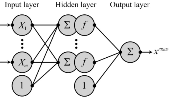
Neural networks (NNs) have become very popular in var-ious scientific areas as a convenient tool for many practi-cal tasks, including time series analysis and data process-ing. Typical artificial neural network is a complex struc-ture, consisting of some number of interconnected, simple signal processing units – artificial neurons (or, shortly, neu-rons). Neurons typically have several inputs and a single output; the information received by inputs is processed by the neuron and the outcome is then transmitted to its neigh-bors. For data processing tasks, so-called feedforward NNs are the ones most frequently applied. A typical feedforward NN consists of several layers of neurons – one, called the input layer, which receives inputs, then one or more hidden layers of signal-processing neurons, and finally, an output layer in which the results are computed to their final form. The output layer can comprise of one or more neurons (pro-ducing one or more output values simultaneously), but we only used single-output networks here. Two different types of feedforward networks were studied in this paper: Multi-Layer Perceptrons (MLPs) and Radial Basis Function (RBF) networks. For more information on NNs, see, e.g. mono-graphs by Haykin (1999) or Principe et al. (2000).

2.2.4 Multilayer perceptron neural networks

MultiLayer Perceptrons (MLPs) are by far the best known and most frequently used design of neural networks – to such an extent that they are sometimes (incorrectly) viewed as be-ing equivalent to NNs generally. The operation performed by neurons in the hidden layer of MLP is a weighted sum-mation. For MLP with one hidden layer and a single neuron in the output layer, the transfer function can be expressed as

xP RED(t ) = v0+ M X i=1 vif w0i+ m X j =1 wj iXj(t ) ! , (6)

Input layer

Hidden layer

Output layer

1

X

X

S

f

S

f

1

x

S

Fig. 2. The schematic structure of multilayer perceptron neural

net-work.

where wj i is the weight of the connection between the i-th neuron in the hidden layer and the j -th neuron in the input layer, viis the weight of the connection between the i-th neu-ron in the hidden layer and the neuneu-ron in the output layer, and

Mis the number of neurons in the hidden layer (structure of a MLP network is schematically shown in Fig. 2). Function

f (x), called the activation function, is generally nonlinear. We used the logistic function,

f (x) = 1

1 + exp (−x). (7)

Apparently, the character of the mapping in Eq. (6) is given by the values of the weights viand wj i, which have to be de-termined before the network can be used. Values of weights are computed using examples of input-output pairs from some training set (supervised learning). The basic learning technique, backpropagation of errors, is an iterative proce-dure using values of errors for the training cases to calcu-late the weights adjustments. The backpropagation technique exists in several variants, differing in their implementation complexity, needed learning time, and tendency to be trapped in a local minimum of the error function instead of reach-ing the global minimum. We have used the quasi-Newton method for MLPs training (e.g. Haykin, 1999), with weights initialized to uniformly distributed random values.

2.2.5 Radial basis function neural networks

In many aspects similar to MLPs, radial basis function neu-ral networks (RBF NNs – Fig. 3) are feedforward networks with one hidden layer and one or more neurons in the output layer. There are two principal differences between MLPs and RBF networks. First, instead of the weighted summation of the inputs, performed by the neurons in the hidden layer of MLPs, RBF networks employ radial basis functions, usually the Gaussian ones. The transfer function can be expressed as

xP RED(t ) = v0+ M X i=1 vi exp − k_{y (t) − ci}k2 2σ_i2 ! , (8)

Input layer Hidden layer Output layer

X

X

1

x

S

Fig. 3. The schematic structure of radial basis function neural

net-work.

where ci is the position of the centre of the i-th radial basis function (assigned to the i-th neuron in the hidden layer, i=1, . . . , M), σi characterizes the width of the i-th RBF, and the meaning of viand M is the same as in Eq. (6).

The second major difference between RBF and MLP neu-ral networks is in the learning algorithm. While weights in MLPs are determined in some sort of iterative learning pro-cedure, training of RBF NNs can be done in two separate phases. First, positions and shapes of the radial basis func-tions are specified (i.e. ci and σi, i=1, . . . , M). The simplest way to do this is to take M randomly chosen times t1, t2, . . . , tM from the training set and use the corresponding vectors in the input space as centres of RBFs, ci=y(ti), i=1, . . . , M. A more sophisticated way of setting ci, k-means clustering (MacQueen, 1967; Haykin, 1999), did not notably improve the results in our case. Values of σi can be set individually for each neuron, but in praxis a single value is often used,

σi=σ, i=1, . . . , M, which we followed. As soon as the po-sitions of RBF centres and sigma are set, finding the values of weights vi, i=0, . . . , M, is a linear problem which can be easily solved using the least-squares approach.

2.3 Computation settings

When testing a time series analysis method, it is important to construct the mapping from one part of the data set, and then to test its performance on an independent interval. For neural networks, the former set is usually referred to as a training set while the latter is called a testing set. We use the same convention for LLM and MLR methods, too.

All utilized nonlinear methods here need one or more pa-rameters to be determined before they can be applied (num-ber of nearest neighbors N for LLM method, num(num-ber of hid-den neurons M for both types of neural networks, width of radial functions σ for RBF networks). The parameters were chosen to give the lowest RMSE for the testing set (a range of parameter values was tested and the best performing one was then used for the actual computation). RMSE depen-dence on the above mentioned parameters typically had a broad, flat minimum and so it was relatively easy to pick

their optimal values. An exception to this rule was observed for the number of hidden neurons in MLPs, when the depen-dence of RMSE on M exhibited notable fluctuations, due to the sensitivity of the results to the initial values of the net-work’s weights. This was compensated for by repeated train-ing (see below), but even then the error curve was visibly less smooth than for RMSE as a function of N or RBF NNs’ M.

Optimization of the parameters was done for the entire year as a whole, not separately for individual seasons. For different tasks, the number of nearest neighbors for the LLM method ranged between 200 and 700. As for the MLP neural networks, the best results were typically obtained with the number of hidden neurons 8 to 12, but sometimes as high as 20. In the case of RBF NNs, the optimal number of hidden units was much higher, usually between 200 and 400. The width of radial functions was set to σ =3.2 (very little sensi-tivity of the results to its value was observed, so we kept it fixed for all tasks). Training of neural networks, both MLP and RBF, was performed 5 times from random initial weights (or RBF centres’ positions, respectively) and the presented results are an average of this five-member ensemble. In ret-rospect, repeated learning was probably not necessary for the RBF networks, since variance of the results within the en-semble was quite low. In the case of MLPs, a single realiza-tion could profoundly misrepresent the performance of the method, so using an entire ensemble was important to reduce the effect of sensitivity to the initial values of weights. Input values for all neural networks were normalized to range [0,1] by subtracting the minimum of the series and then dividing the value with the series’ max-min range. MLP networks were trained for 1500 epochs by the quasi-Newton method.

An important part of the input data is information about the season of the year. In order to introduce this informa-tion to the computainforma-tions, applicainforma-tion of the MLR and LLM methods was done separately for each season. For NNs, we did perform the training for the entire training set as a whole, and information about the season was introduced by four ex-tra neurons in the input layer, each of which was assigned to one season (the effective dimension of the input space was therefore m=18 for all neural networks). These neurons’ ac-tivations were equal to 1 for the season they controlled, and 0 otherwise (i.e. just one of these four neurons was active for a given time – the one assigned to the corresponding season). Another possibility of introducing information about the sea-son would be using sine and cosine of the Julian day (as done by Trigo and Palutikof, 1999). The usual climatological def-inition of the seasons was utilized:

Winter =December + January + February =DJF, Spring =March + April + May =MAM, Summer = June + July + August =JJA and Autumn = September + October + November = SON .

3 Data

The first data set utilized was the NCEP/NCAR reanalysis by Kistler et al. (2001), obtained from the page of

NOAA-CIRES CDC at http://www.cdc.noaa.gov. It is available for the years from 1948 on, and it covers an entire world with reanalysis of several meteorological variables in the regu-lar 2.5◦×2.5◦grid, including data for various pressure lev-els. Series of mean daily temperature at the level 1000 hPa (T1000)were used here, as well as series of mean sea level pressure (MSLP) and series of geopotential height of the 500 hPa level (h500).

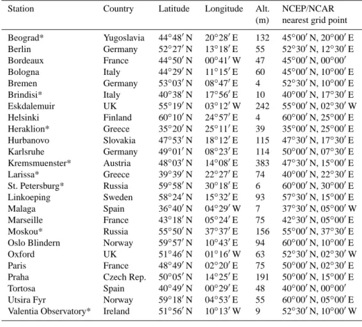
As for directly measured meteorological series, perhaps the largest publicly available data set of European tempera-ture, precipitation and pressure measurements was collected by Klein Tank et al. (2002) and it is obtainable from the In-ternet page of the European Climate Assessment and Dataset (ECA&D – http://eca.knmi.nl/). Measurements from many different sources were assembled by the authors, so series of various quality and length are part of ECA&D, and many of them contain missing values. We used series of daily mean, minimum and maximum temperature from 25 European sta-tions – see Table 1 for their list. Many more series can be obtained from ECA&D – these 3×25 were selected in order to cover most of Europe with series available for the years 1961 to 2000, or ending not too long before the year 2000, and containing as little missing values as possible.

4 Results 4.1 Prediction

Forecast of future weather is what most people view as a fun-damental purpose of meteorology’s existence. And although today’s weather forecasts are made almost exclusively by means of numerical models, there are many supplementary tasks for which time series analysis can be more suitable, for example, because the available data do not allow for use of a generally demanding NWF model, because of unsuit-able spatial or temporal scale or due to a lack of availunsuit-able computing capacity. It was shown that nonlinear methods can be applied for tasks like prediction of road temperatures (Shao, 1998), precipitation forecasting (Waelbroeck et al., 1994; Hall et al., 1999; Sivakumar et al., 2000), or forecast of cloud cover (P´erez-Mu˜nuzuri and Gelpi, 2000), although in some cases nonlinear methods do not seem to be more suit-able than the linear ones, as demonstrated, for example, by Tang et al. (2000) for Central Pacific SST forecast.

The gridded NCEP/NCAR reanalysis data set represents a suitable basis for study of spatial distribution of the pre-dictive potential of nonlinear methods. First, we performed the prediction of the T1000series one day ahead by the LLM and MLR methods for every grid point in the area between 65◦N, 25◦W and 25◦N, 45◦E, i.e. for 493 points in total. Years 1961–1990 were used as the training set, while the test-ing set consisted of the years 1991–2000. The structure of the predictor space is demonstrated in Fig. 1a for the grid point 50◦N, 15◦E (the pattern was moved to be centered on the location of the predicted series). Unlike for all the other computations in this paper, a fixed number of nearest

Table 1. A list of stations used for downscaling tests. Asterisk (*) marks the stations for which at least one of the series of daily mean,

minimum or maximum temperature did not cover the entire period 1961–2000.

Station Country Latitude Longitude Alt. NCEP/NCAR

(m) nearest grid point Beograd* Yugoslavia 44◦480N 20◦280E 132 45◦000N, 20◦000E Berlin Germany 52◦270N 13◦180E 55 52◦300N, 12◦300E Bordeaux France 44◦500N 00◦410W 47 45◦000N, 00◦000 Bologna Italy 44◦290N 11◦150E 60 45◦000N, 10◦000E Bremen Germany 53◦030N 08◦470E 4 52◦300N, 10◦000E Brindisi* Italy 40◦380N 17◦560E 10 40◦000N, 17◦300E Eskdalemuir UK 55◦190N 03◦120W 242 55◦000N, 02◦300W Helsinki Finland 60◦100N 24◦570E 4 60◦000N, 25◦000E Heraklion* Greece 35◦200N 25◦110E 39 35◦000N, 25◦000E Hurbanovo Slovakia 47◦530N 18◦120E 115 47◦300N, 17◦300E Karlsruhe Germany 49◦010N 08◦230E 114 50◦000N, 07◦300E Kremsmuenster* Austria 48◦030N 14◦080E 383 47◦300N, 15◦000E Larissa* Greece 39◦390N 22◦270E 74 40◦000N, 22◦300E St. Petersburg* Russia 59◦580N 30◦180E 6 60◦000N, 30◦000E Linkoeping Sweden 58◦240N 15◦320E 93 57◦300N, 15◦000E Malaga Spain 36◦400N 04◦290W 7 37◦300N, 05◦000W Marseille France 43◦180N 05◦240E 75 42◦300N, 05◦000E Moskou* Russia 55◦500N 37◦370E 156 55◦000N, 37◦300E Oslo Blindern Norway 59◦570N 10◦430E 94 60◦000N, 10◦000E Oxford UK 51◦460N 01◦160W 63 52◦300N, 02◦300W Paris France 48◦490N 02◦200E 75 50◦000N, 02◦300E Praha Czech Rep. 50◦050N 14◦250E 191 50◦000N, 15◦000E Tortosa Spain 40◦490N 00◦290E 48 40◦000N, 00◦000 Utsira Fyr Norway 59◦180N 04◦530E 55 60◦000N, 05◦000E Valentia Observatory* Ireland 51◦560N 10◦130W 9 52◦300N, 10◦000W

Winter Summer

Fig. 4. RMSE (◦C) of 1-day ahead prediction of temperature at the 1000 hPa level (T1000)by LLM method. Three black crosses mark the positions of the grid points from Table 2.

neighbors was used for all grid points, N =250. The results are shown in Fig. 4 (RMSE for LLM method) and 5 (RMSE for LLM method, divided with RMSE for MLR, which we will call effective nonlinearity, since it quantifies an improve-ment which can be gained from replacing linear MLR with the nonlinear method of local models).

The lowest values of RMSE were detected over the Mediterranean Sea and Atlantic Ocean, and, in summer, in the Near East. Errors in summer were generally lower than in winter. The absolute values of the errors coincide well with values of average interdiurnal temperature change, i.e. errors were higher in the areas with higher temperature vari-ability. When the spatial structure of effective nonlinearity

was analyzed, the observed pattern was more complex. In winter, most of continental Europe appears to be a region of increased nonlinearity, with the highest differences between RMSE for the LLM and MLR methods in Western Europe and Russia. Nonlinearity seems to be rather weak in the mar-itime areas, as well as in Northern Africa and the Near East. In summer, nonlinearity is weaker than in winter in most ar-eas, and there is a clear contrast between the Mediterranean area (very weak nonlinearity, except for Tunisia and North-ern Libya) and the rest of Europe (rather stronger nonlin-earity, especially in Northern France, Belgium and Nether-lands). This observed pattern bears an interesting resem-blance to the positions of the climatic zones, as nonlinearity

Table 2. RMSE (◦C) of 1-day ahead prediction of NCEP/NCAR T₁₀₀₀series for three different grid points. The values in bold indicate that the nonlinear method gave better results than multiple linear regression, according to the paired Wilcoxon test at the 95% confidence level. The values in the first row show RMSE of persistent prediction.

50◦N, 0◦E 50◦N, 15◦E 40◦N, 15◦E

DJF MAM JJA SON DJF MAM JJA SON DJF MAM JJA SON Pers. 2.12 1.8 1.73 1.74 2.73 2.41 2.31 2.31 1.42 1.15 0.99 1.23 MLR 1.75 1.48 1.3 1.5 2.3 1.9 1.65 1.86 1.11 0.98 0.83 0.99 LLM 1.41 1.28 1.07 1.21 1.93 1.57 1.44 1.54 0.96 0.88 0.83 0.88 MLP 1.52 1.35 1.18 1.24 1.9 1.54 1.46 1.57 0.98 0.92 0.81 0.89 RBF 1.39 1.26 1.07 1.15 1.87 1.52 1.38 1.54 0.95 0.87 0.79 0.88 Winter Summer

Fig. 5. Effective nonlinearity for 1-day ahead prediction of temperature at the 1000 hPa level (T₁₀₀₀), i.e. RMSE for LLM method expressed in % of RMSE for multiple linear regression (lower values indicate stronger nonlinearity). Three black crosses mark the positions of the grid points from Table 2.

seems to be stronger in the temperate zone and weaker in the subtropical and tropical areas (various climate classifications can be found in Essenwanger, 2001).

There is a comparison of 1-day ahead prediction results in Table 2 for all tested methods and all seasons of the year for three selected NCEP/NCAR grid points: 50◦N, 0◦E (a grid point which exhibited strong effective nonlinearity in both summer and winter), 50◦N, 15◦E (medium nonlinearity in both seasons) and 40◦N, 15◦E (medium nonlinearity in win-ter, very weak in summer). Positions of the respective grid points are indicated by crosses in Figs. 4 and 5. Aside from comparing RMSEs, differences between individual methods were ascertained using the paired Wilcoxon test (e.g. Wilks, 1995), applied at the absolute values of daily errors. The significance of the differences between errors from the MLR and nonlinear methods is indicated in Table 2 – values in bold signal that the nonlinear method was better than MLR at the 95% level of confidence. RBF NN typically gave the best results of all three nonlinear methods in terms of RMSE, but the difference of error medians was not significant, accord-ing to the Wilcoxon test, in most of the tested cases. On the other hand, nonlinear methods, especially LLM and RBF NNs, typically gave better results than MLR, both with re-spect to RMSE and to the significance of the difference of daily errors.

Visually, there was just little difference between the series of predictions from all four tested methods. Superiority of nonlinear techniques in the geographic areas with strong

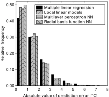
ef-0 1 2 3 4 5 6 7 8

Absolute value of prediction error [°C] 0.00 0.10 0.20 0.30 0.40 0.50 R el at iv e fr eq ue nc y

Multiple linear regression Local linear models Multilayer perceptron NN Radial basis function NN

Fig. 6. Histogram of the absolute values of the prediction errors

for 1-day ahead prediction of NCEP/NCAR T1000series at 50◦N, 15◦E (whole year).

fective nonlinearity was, however, clearly visible in the dis-tribution of errors, with residuals close to zero being rela-tively more frequent for nonlinear methods than for MLR – see example in Fig. 6. What all methods had in com-mon was a certain tendency to underestimate high values of temperature and overestimate the low ones, thus actually

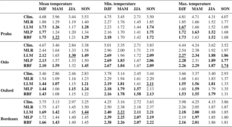
Table 3. RMSE (◦C) of NCEP/NCAR reanalysis downscaling for four European stations. The values in bold indicate that the nonlinear method gave better results than multiple linear regression, according to the Wilcoxon test at the 95% confidence level. Underline indicates that the method performed better than all the other three, according to the Wilcoxon test. The values in the first row for each station show RMSE obtained by means of mean climatology.

Mean temperature Min. temperature Max. temperature

DJF MAM JJA SON DJF MAM JJA SON DJF MAM JJA SON

Praha Clim. 4.68 3.96 3.44 3.53 4.75 3.45 2.71 3.50 4.81 4.71 4.31 4.07 MLR 1.88 1.29 1.19 1.40 2.27 1.76 1.45 1.85 1.85 1.66 1.52 1.77 LLM 1.73 1.26 1.17 1.28 2.23 1.72 1.44 1.74 1.67 1.66 1.52 1.69 MLP 1.77 1.24 1.20 1.34 2.16 1.70 1.41 1.75 1.72 1.63 1.52 1.68 RBF 1.75 1.22 1.21 1.29 2.18 1.70 1.42 1.72 1.73 1.63 1.52 1.68 Oslo Clim. 4.67 3.46 2.84 3.38 5.01 3.35 2.71 3.83 4.44 4.24 3.62 3.52 MLR 2.44 1.64 1.33 1.58 2.96 2.00 1.71 2.19 2.54 2.38 1.92 1.97 LLM 2.12 1.65 1.30 1.49 2.69 1.96 1.72 2.09 2.27 2.34 1.88 1.86 MLP 2.13 1.57 1.33 1.50 2.69 1.83 1.67 2.06 2.28 2.31 1.89 1.77 RBF 2.10 1.59 1.32 1.45 2.67 1.84 1.67 2.09 2.26 2.29 1.87 1.74 Oxford Clim. 3.46 2.86 2.46 2.83 3.78 3.14 2.45 3.44 3.66 3.37 3.40 2.93 MLR 1.54 1.09 1.16 1.23 2.29 1.94 1.61 2.20 1.68 1.61 1.83 1.37 LLM 1.44 1.07 1.15 1.21 2.19 1.81 1.61 2.11 1.55 1.56 1.81 1.33 MLP 1.44 1.06 1.15 1.24 2.18 1.79 1.57 2.13 1.60 1.59 1.79 1.35 RBF 1.43 1.08 1.15 1.22 2.16 1.78 1.58 2.13 1.53 1.55 1.79 1.31 Bordeaux Clim. 3.75 3.13 2.97 3.25 4.25 3.16 2.72 3.63 3.98 4.25 4.15 3.86 MLR 1.75 1.47 1.45 1.50 2.50 2.38 2.18 2.37 2.26 2.05 1.87 1.87 LLM 1.69 1.42 1.45 1.44 2.40 2.22 2.11 2.21 2.18 2.00 1.88 1.85 MLP 1.72 1.44 1.40 1.45 2.39 2.25 2.07 2.19 2.19 1.97 1.85 1.80 RBF 1.66 1.43 1.40 1.45 2.38 2.26 2.07 2.22 2.16 2.01 1.86 1.81

Fig. 7. Plot of the prediction residuals (the predicted temperature

minus the original observed temperature) against the original tem-perature for 1-day ahead prediction of NCEP/NCAR T1000series at 50◦N, 15◦E (whole year). Bold line represents the linear fit of the residuals.

decreasing the variance of the series of predictions compared to the original one. This kind of behavior was observed for all seasons, as well as the year as a whole, and it is demon-strated for the grid point 50◦N, 15◦E in Fig. 7. The problem of a deformed distribution of values is commonly

encoun-tered in the context of the application of empirical models in climate research, particularly in statistical downscaling, and various strategies have been proposed for handling it, such as variance inflation or partial randomization (e.g. von Storch, 1999). All results presented here are direct outputs of the transfer functions, without being subject to any form of ad-ditional postprocessing.

4.2 Downscaling

Statistical downscaling of large-scale data is another com-mon task of meteorological time series analysis, and one in which nonlinear methods are sometimes used. Several studies have been published devoted to downscaling or post-processing of temperatures by nonlinear methods, mostly MLPs (Trigo and Palutikof, 1999; Schoof and Pryor, 2001; Marzban, 2003; Casaioli et al., 2003) or neural networks based on RBF functions (Weichert and B¨urger, 1998). Here, downscaling of the gridded large-scale data was done for the predictand series of daily mean, minimum and maximum temperatures. NCEP/NCAR reanalysis series were used as predictors. The pattern of predictors (Fig. 1b) was centered on the NCEP/NCAR grid point closest to the respective sta-tion (see the last column of Table 1). Years 1961–1990 were used as the training set, and years 1991–2000 as the testing set. In some cases, the testing set was shorter than 10 years

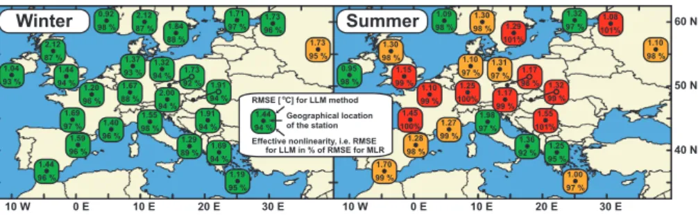
0.92 98 % 1.04 93 % 2.12 87 % 1.44 94 % 1.73 95 % 1.73 96 % 1.71 97 % 2.12 87 % 1.84 88 % 1.37 93 % 1.67 88 % 1.20 96 % 1.69 97 % 1.59 96 % 1.44 96 % 1.40 96 % 1.55 98 % 1.29 89 % 1.69 94 % 1.19 95 % 1.91 94 % 1.32 94 % 2.00 94 % 1.73 92 % 1.91 94 % 1.09 98 % 0.95 98 % 1.30 98 % 1.15 99 % 1.10 98 % 1.08 101% 1.32 97 % 1.30 98 % 1.29 101% 1.10 97 % 1.25 100% 1.10 99 % 1.45 100% 1.28 98 % 1.70 99 % 1.27 99 % 1.98 97 % 1.36 92 % 1.25 95 % 1.00 97 % 1.55 101% 1.31 97 % 1.17 99 % 1.17 98 % 1.32 99 % Winter Summer

Effective nonlinearity, i.e. RMSE for LLM in % of RMSE for MLR

1.44

94 % Geographical location of the station RMSE [ C] for LLM methodo

60 N

50 N

40 N

10 W 0 E 10 E 20 E 30 E 10 W 0 E 10 E 20 E 30 E

Fig. 8. Results of NCEP/NCAR reanalysis downscaling by LLM and MLR methods for 25 European stations – daily mean temperature.

Color of the station’s background shows the result of the test of the hypothesis that the absolute values of daily errors were the same for both methods, against the alternative that errors were smaller for LLM – red means that the hypothesis was not rejected at the level of confidence of 95%, yellow that it was rejected at 95%, but not at 99%, and green means that the difference or errors was significant at the 99% level of confidence (one-sided paired Wilcoxon test was used).

Winter 1.13 Summer 98 % 1.79 94 % 2.53 92 % 2.19 95 % 2.65 96 % 2.63 97 % 2.41 96 % 2.69 91 % 2.78 91 % 2.15 98 % 2.43 94 % 1.56 94 % 2.40 96 % 2.22 93 % 2.32 95 % 1.84 93 % 2.26 98 % 2.07 92 % _{97 %}2.79 2.48 96 % 2.15 100% 1.92 100% 2.49 98 % 2.23 98 % 2.77 100% 1.22 98 % 1.56 98 % 2.22 98 % 1.61 100% 1.66 100% 1.47 100% 1.57 98 % 1.72 101% 1.99 99 % 1.96 98 % 1.64 99 % 1.21 99 % 2.11 97 % 1.36 99 % 1.80 101% 1.47 98 % 1.63 98 % 1.72 98 % _100%2.03 1.87 100% 1.57 97 % 1.71 99 % 1.64 99 % 1.44 99 % 1.77 98 %

Effective nonlinearity, i.e. RMSE for LLM in % of RMSE for MLR

1.44 94 %

Geographical location of the station RMSE [ C] for LLM methodo

60 N

50 N

40 N

10 W 0 E 10 E 20 E 30 E 10 W 0 E 10 E 20 E 30 E

Fig. 9. Same as Fig. 8, for daily minimum temperature.

because the predictand temperature series was not available for the whole interval (such stations are marked with an as-terisk in Table 1). Moreover, some of the series contained missing values – in those cases, the respective days were ex-cluded from the computation. The number of missing values was, however, always very small in comparison with the total size of the data set, so their presence should not have caused any major shift in the results.

For all 25 stations from Table 1, results of downscaling by MLR and LLM methods for daily mean (Fig. 8), mini-mum (Fig. 9) and maximini-mum (Fig. 10) temperature in win-ter and in summer are presented. Aside from computing the relative differences between RMSE for the LLM and MLR methods, we also tested the statistical significance of the dif-ference of the medians of the absolute values of daily errors for the LLM and MLR methods. The testing was done by the one-sided paired Wilcoxon test, and its outcomes are repre-sented by different colors of the respective station’s back-ground in Figs. 8 to 10. Full results for the four stations are shown in Table 3. Situations when nonlinear method gave better results than MLR at the 95% level of confidence are indicated by bold print. To compare the results to outcomes of a low-skill method, the table also contains RMSE obtained by means of mean climatology (i.e. when monthly mean val-ues of the predictand were used in the role of xP RED(t )from Eq. (3)).

Nonlinear methods generally performed better than MLR, but there were distinct differences between the seasons – most profoundly nonlinear behavior was typical for winter,

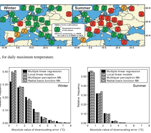
while in summer, nonlinear techniques seemed to grant just a very small, if any, improvement in the comparison with MLR at most stations. This can be easily seen from Fig. 11, where histograms of the absolute values of downscaling er-rors are shown for mean daily temperature from Oslo (a sta-tion, where the contrast between winter and summer was par-ticularly clear). A tendency was observed in all methods to underestimate high temperatures and overestimate the low ones, as in the case of the forecasts in Sect. 4.1.

Situations when one of the methods was superior to all the others, according to the Wilcoxon test, were rather rare, and they are marked with an underline in Table 3. None of the nonlinear methods could be identified as the best one in all cases, or the majority of the cases. However, when one of the methods was tested as the best performing one, it was usually either the method of local models or the RBF neural network.

Unlike the forecasts studied in Sect. 4.1, results of down-scaling were influenced by local conditions of individual sta-tions and by eventual problems with series quality (shorter length of some series, as well as the fact that the series in ECA&D were collected from many different sources, and they may not be mutually as easily comparable as NCEP/NCAR reanalysis data). Thus, we have not tried to draw any detailed conclusions about the geographical struc-ture of errors or nonlinearity based on the behavior of indi-vidual stations. A few points can be made, nonetheless:

Winter 1.00 Summer 96 % 0.95 94 % 1.51 93 % 1.55 92 % 1.83 97 % 1.80 96 % 1.84 96 % 2.27 89 % 1.55 92 % 1.46 96 % 2.14 96 % 1.74 98 % 2.18 97 % 2.07 98 % 1.51 98 % 1.61 99 % 3.42 98 % 1.32 95 % _{93 %}2.23 1.57 97 % 2.66 94 % 1.49 96 % 2.16 90 % 1.67 90 % 2.49 94 % 1.30 96 % 1.18 94 % 1.82 95 % 1.81 99 % 1.75 100% 1.65 101% 1.35 99 % 1.88 98 % 1.70 102% 1.59 100% 1.94 101% 1.89 99 % 1.88 100% 1.99 98 % 2.49 99 % 1.79 100% 2.80 98 % 1.75 94 % 1.44_{98 %} 1.48 97 % 1.96 102% 1.63 99 % 1.60 100% 1.52 100% 1.85 102%

Effective nonlinearity, i.e. RMSE for LLM in % of RMSE for MLR

1.44 94 %

Geographical location of the station RMSE [ C] for LLM methodo

60 N

50 N

40 N

10 W 0 E 10 E 20 E 30 E 10 W 0 E 10 E 20 E 30 E

Fig. 10. Same as Fig. 8, for daily maximum temperature.

0.00 0.10 0.20 0.30 0.40 0.50 0 1 2 3 4 5 6 7 8 Multiple linear regression Local linear models Multilayer perceptron NN Radial basis function NN

0 1 2 3 4 5 6 7 8 0.00

0.10 0.20 0.30

0.40 Multiple linear regression Local linear models Multilayer perceptron NN Radial basis function NN

Absolute value of downscaling error (°C)

R el at iv e fr eq ue nc y _Winter

Absolute value of downscaling error (°C)

R el at iv e fr eq ue nc y _Summer

Fig. 11. Histogram of the absolute values of downscaling errors for mean daily temperature from Oslo, Norway, in winter (left) and summer

(right).

– Values of RMSE were higher in winter than in summer at most stations, for mean and minimum temperatures; for maximum temperature, almost half of the stations showed higher values of error in summer. The effec-tive nonlinearity was typically stronger in winter than in summer for all three types of temperature. In sum-mer, nonlinear methods even performed a little worse than MLR sometimes, and for many stations, the differ-ence in the medians of errors was not conclusive at the confidence level of 95%.

– Errors were lower for daily mean temperatures than for maximum or minimum ones in most locations. This is not surprising as mean values are already averaged in time, and therefore smoother. The extreme temperatures represent values in a single moment during the day, hence they are more prone to be affected with a noise component of the atmospheric dynamics, and more dif-ficult to determine.

– In Sect. 4.1, we pointed out that nonlinearity in the Mediterranean area seems to be significantly weaker than for the rest of Europe. Here, a similar rule does not apply and there is no clear connection between the geographic position of the station and the degree of ex-hibited nonlinearity, as even geographically close sta-tions exhibited quite a different behavior in a number of cases.

5 Discussion

The presented analyses, carried out for different tasks and various series, do not identify any of the tested nonlinear methods to be definitely superior to the others. It is, however, obvious that in most cases the LLM, MLP NN and RBF NN methods outperformed multiple linear regression. Applica-tion of nonlinear methods seems, therefore, to be useful for meteorological time series analysis at synoptic time scales, but the issue remains as to which one of them should be used preferably. Aside from the performance itself, attention should also be paid to the application properties of the con-testants. Advantages and drawbacks of individual methods may be summarized as follows:

– Method of local linear models’ advantage is that its use need not be preceded by the potentially time-consuming training of weights. On the other hand, the execution itself takes longer than for the already trained NNs, due to the search for nearest neighbors, which needs to be carried out for every processed state. This method is faster than both types of NNs when applied just once for a given setting, as we did in order to obtain the results for Figs. 4 and 5. Its speed also makes estimation of suitable parameters (specifically, N ) by a trial-and-error technique easier.

– MLPs are the most frequently used nonlinear technique of the tested ones, which is an advantage by itself, due

to support in many existing software applications. Their features are well documented and thoroughly discussed by a number of authors (among others Haykin, 1999; Principe et al., 2000). Perhaps the most severe draw-back of MLPs is the possibility that the learning proce-dure will end in a local minimum of the error function instead of reaching the global one. The seriousness of this problem can be reduced by means of repeated train-ing or by application of a global minimum search tech-nique (such as the one used by Casaioli et al., 2003), but usually at the cost of increased training time. There is also the possibility of overtraining, when the learn-ing procedure runs for too long a time, and the network becomes overoptimized for the description of the cases from the learning set, thus losing its ability to gener-alize. None of these problems is unsolvable, but they cause the application of MLPs to be potentially tricky, with many nontrivial decisions to be made and the learn-ing process which needs to be supervised.

– RBF NNs do not suffer from the “local minimum trap” problem (at least not their form that we used here), be-cause the supervised optimization of the weights to the output layer can be treated as a linear problem. Certain variations of the results can arise from the random se-lection of the RBF centers, but these were very small in our case. There is also no need to worry about the net-work becoming overtrained. Nonetheless, it is still pos-sible to overfit the network in the sense of too many free parameters (when too many hidden neurons are used). Training of RBF NNs is usually faster than that of MLPs (especially considering the need for repeated training of MLPs).

Therefore, the RBF NNs and LLM method can offer better application properties than MLPs in many respects. Consid-ering their relatively easy implementation, we believe that these methods can be recommended as a worthy alternative to MLPs.

The error and nonlinearity maps in Figs. 4, 5 and 8 to 10 offer some insight into the geographic structure of spatiotem-poral relations between the atmospheric variables, but they should be interpreted carefully. For prediction (Figs. 4 and 5), the fact that the reanalysis and not measured data was used may be partly responsible for the character of the ob-served structures. There is also an issue of selection of the input variables – the presented results were obtained for one specific pattern of predictors, and it can be argued that the maps could change if a different one was used. We repeated the tests for various sets of predictors, differing in both type and number of variables used, and although the details of the maps changed, the basic geographic structure of nonlinearity seemed quite robust and unaffected by the modification of the computation settings. There still was an area of distinct nonlinearity over continental Europe, more apparent in win-ter than in summer, while over the Mediwin-terranean and North-ern Africa, nonlinearity was weaker. These results suggest

that the nonlinear character of the climate system is strongly reflected in the atmospheric time series in the midlatitudes, and that the relations between them cannot be fully described by linear mappings. In the tropical areas south of Europe, a purely linear description seems more sufficient.

Interpretation of the downscaling tests needs to be done with respect to their possible dependence on the tested sta-tions’ local conditions. The observed profound differences between even close stations suggest that conclusions about the skill and suitability of time series analysis methods, ob-tained for a limited area or a single station, cannot be au-tomatically generalized and applied to different locations. Noteworthy is the seasonal variance of the results, which im-plies the presence of a strong detectable nonlinear component in the relations between predictors and predictand in winter, and a rather linear character of these relations in summer.

It is also interesting that the effective nonlinearity is gener-ally weaker for downscaling than for forecasting tasks (com-pare results in Figs. 5 and 8). This does not necessarily mean that the relations between predictors and predictand are in-trinsically more linear in the case of downscaling. The reason for this difference may lie in the fact that while the forecast-ing tests were done solely on reanalysis data, which are rel-atively smooth by construction, downscaling predictands are local measurements. They reflect the situation in just a very small area, so it is possible for them to contain a stronger high-dimensional component, which may be nonlinear in its nature, but has a character of noise and is too complex to be described by any time series analysis method, even a nonlin-ear one.

6 Conclusions

Our primary intention was to make a comparison of three nonlinear methods and to identify the one most suitable for the analysis of climatic data at synoptic time scales. It turned out that the most commonly applied nonlinear method, multi-layer perceptron neural network, may not necessarily be the best possible choice. The other two tested nonlinear tech-niques, method of local linear models and radial basis func-tion neural network, performed equally well, even better in many cases, they do not suffer from MLPs’ drawbacks, such as the problem of local minima of the error function or the danger of overtraining, and their implementation is relatively easy. We can therefore recommend them as a worthy alter-native to MLPs.

The constructed maps of the geographical structure of er-rors and effective nonlinearity revealed profound spatial vari-ations of the results. In case of prediction, a distinct con-trast between the temperate zone (stronger nonlinearity) and the subtropical and tropical zones (weaker nonlinearity) was found, especially in summer. As for downscaling tests, we were not able to identify any apparent large-scale geograph-ical distribution of nonlinearity, probably because the results for individual stations were influenced by the local condi-tions at least as much as by the large-scale climate dynamics.

For both forecasting and downscaling, profound seasonal dependence of the results was observed, with errors being larger and nonlinearity being stronger in winter than in sum-mer in most locations.

Acknowledgements. This work was supported by the Grant Agency

of Charles University, grant 227/2002/B-GEO/MFF, Ministry of the Environment of the Czech Republic, grant VaV/740/2/03 and Research project 113200004. We would also like to express our gratitude to B. Sivakumar for his valuable comments on the manuscript, and to thank the two anonymous reviewers of the previous version of the manuscript.

Edited by: A. Tsonis Reviewed by: B. Sivakumar

References

Abarbanel, H. D. I.: Analysis of Observed Chaotic Data. Springer, New York, 272 pp., 1996.

Casaioli, M., Mantovani, R., Scorzoni, F. P., Puca, S., Speranza, A., and Tirozzi, B.: Linear and nonlinear post-processing of numer-ically forecasted surface temperature, Nonlin. Processes Geo-phys., 10, 373–383, 2003,

SRef-ID: 1607-7946/npg/2003-10-373.

Essenwanger, O. M.: General Climatology: Classification of Cli-mates (World Survey of Climatology, Vol. 1 Part C), Elsevier, Amsterdam, 113 pp., 2001.

Farmer, J. D. and Sidorowich, J. J.: Predicting Chaotic Time Series, Phys. Rev. Lett., 59, 845–847, 1987, reprinted in Ott et al. (1994). Fraedrich, K.: Estimating the Dimensions of Weather and Climate

Attractors, J. Atmos. Sci., 43, 419–432, 1986.

Galka, A.: Topics in Nonlinear Time Series Analysis – With Im-plications for EEG Analysis, World Scientific Publishing, Singa-pore, 342 pp., 2000.

Hall, T., Brooks, H. E., and Doswell, C. A.: Precipitation Forecast-ing UsForecast-ing a Neural Network, Weather Forecast., 14, 338–345, 1999.

Haykin, S.: Neural networks: A comprehensive foundation (2nd edition), Prentice Hall, Upper Saddle River, New Jersey, 842 pp., 1999.

Hegger, R., Kantz, H., and Schreiber, T.: Practical implementa-tion of nonlinear time series methods: The TISEAN package, CHAOS, 9, 413–435, 1999.

Huth, R.: Statistical Downscaling of Daily Temperature in Central Europe, J. Climate, 15, 1731–1742, 2002.

Huth, R.: Sensitivity of Local Daily Temperature Change Estimates to the Selection of Downscaling Models and Predictors, J. Cli-mate, 17, 640–652, 2004.

Jayawardena, A. W. and Gurung, A. B.: Noise reduction and predic-tion of hydrometeorological time series: dynamical systems ap-proach vs. stochastic apap-proach, J. Hydrol., 228, 242–264, 2000. Jayawardena, A. W., Li, W. K., and Xu, P.: Neighbourhood

se-lection for local modelling and prediction of hydrological time series, J. Hydrol., 258, 40–57, 2002.

Kantz, H. and Schreiber, T.: Nonlinear time series analysis. Cam-bridge University Press, CamCam-bridge, 304 pp., 1997.

Keppenne, C. L. and Nicolis, C.: Global Properties and Local Struc-ture of the Weather Attractor over Western Europe, J. Atmos. Sci., 46, 2356–2370, 1989.

Kistler, R., Kalnay, E., Collins, W., Saha, S., White, G., Woollen, J., Chelliah, M., Ebisuzaki, W., Kanamitsu, M., Kousky, V., van den Dool, H., Jenne, R., and Fiorino, M.: The NCEP–NCAR 50– Year Reanalysis: Monthly Means CD-ROM and Documentation, B. Am. Meteorol. Soc., 82, 247–268, 2001.

Klein Tank, A. M. G., Wijngaard, J. B., K¨onnen, G. P., et al.: Daily dataset of 20th-century surface air temperature and precipitation series for the European Climate Assessment, Int. J. Climatol., 22, 1441–1453, 2002.

MacQueen, J.: Some methods for classification and analysis of multivariate observations, Proceedings of the 5th Berkeley Sym-posium on Mathematical Statistics and Probability, 1, 281–297, 1967.

Marzban, C.: A Neural Network for Post-processing Model Output: ARPS, Mon. Weather Rev., 131, 1103–1111, 2003.

Miksovsky, J. and Raidl, A.: Testing for nonlinearity in European climatic time series by the method of surrogate data, Theor. Appl. Climatol., in press, 2005.

Ott, E., Sauer, T., and Yorke, J. A. (eds.): Coping with chaos: Anal-ysis of chaotic data and the exploitation of chaotic systems, John Wiley & Sons, New York, 418 pp., 1994.

Packard, H. N., Crutchfield, J. P., Farmer, J. D., and Shaw, R. S.: Geometry from a time series, Phys. Rev. Lett., 45, 712–716, 1980, reprinted in Ott et al. (1994).

Palus, M.: Detecting nonlinearity in multivariate time series, Phys. Lett. A, 213, 138–147, 1996.

Palus, M. and Novotna, D.: Testing for nonlinearity in weather records, Phys. Lett. A, 193, 67–74, 1994.

P´erez-Mu˜nuzuri, V. and Gelpi, I. R.: Application of nonlinear fore-casting techniques for meteorological modeling, Ann. Geophys., 18, 1349–1359, 2000,

SRef-ID: 1432-0576/ag/2000-18-1349.

Principe, J. C., Euliano, N. R., and Lefebvre, W. C.: Neural and Adaptive systems: Fundamentals through Simulations, John Wi-ley & Sons, New York, 656 pp., 2000.

Sauer, T.: Time Series Prediction by Using Delay Coordinate Em-bedding., in: Time Series Prediction: Forecasting the Future and Understanding the Past, Santa Fe Institute Studies in the Science of Complexity XV, edited by: Weigend, A. S. and Gershenfeld, N. A., Addison-Wesley, Reading, 643 pp., 1993, reprinted in Ott et al. (1994).

Schoof, J. T. and Pryor, S. C.: Downscaling temperature and precip-itation: A comparison of regression-based methods and artificial neural networks, Int. J. Climatol., 21, 773–790, 2001.

Schreiber, T. and Schmitz, A.: Surrogate time series, Physica D, 142, 346–382, 2000.

Shao, J.: Improving Nowcasts of Road Surface Temperature by a Backpropagation Neural Network, Weather Forecast., 13, 164– 171, 1998.

Sivakumar, B.: Chaos theory in geophysics: past, present and fu-ture, Chaos Soliton. Fract., 19, 441–462, 2004.

Sivakumar, B., Berndtsson, R., Olsson, J., Jinno, K., and Kawa-mura, A.: Dynamics of monthly rainfall-runoff process at the G¨ota basin: A search for chaos, Hydrol. Earth Syst. Sci., 4, 407– 417, 2000,

SRef-ID: 1607-7938/hess/2000-4-407.

Sugihara, G. and May, R. M.: Nonlinear forecasting as a way of dis-tinguishing chaos from measurement error in time series, Nature, 344, 734–740, 1990, reprinted in Ott et al. (1994).

Takens, F.: Detecting Strange Attractors in Turbulence, in: Dynami-cal Systems and Turbulence, Lecture Notes in Mathematics, Vol. 898, edited by: Rand, D. A and Zouny, L. S., Springer, New

York, 366–381, 1981.

Tang, B., Hsieh, W. W., Monahan, A. H., and Tangang, F. T.: Skill Comparisons between Neural Networks and Canonical Correla-tion Analysis in Predicting the Equatorial Pacific Sea Surface Temperatures, J. Climate, 13, 287–293, 2000.

Trigo, R. M. and Palutikof, J. P.: Simulation of daily temperatures for climate change scenarios over Portugal: a neural network model approach, Climate Res., 13, 45–59, 1999.

Tsonis, A. A.: Probing the linearity and nonlinearity in the transi-tions of the atmospheric circulation, Nonlin. Processes Geophys., 8, 341–345, 2001,

SRef-ID: 1607-7946/npg/2001-8-341

von Storch, H.: On the Use of “Inflation” in Statistical Downscal-ing, J. Climate, 12, 3505–3506, 1999.

Waelbroeck, H., L´opez-Pe˜na, R., Morales, T., and Zertuche, F.: Pre-diction of Tropical Rainfall by Local Phase Space Reconstruc-tion, J. Atmos. Sci., 51, 3360–3364, 1994.

Weichert, A. and B¨urger, G.: Linear versus nonlinear techniques in downscaling, Climate Res., 10, 83–93, 1998.

Wilks, D. S.: Statistical methods in the atmospheric sciences, Aca-demic Press, San Diego, 467 pp., 1995.