HAL Id: hal-00296545
https://hal.archives-ouvertes.fr/hal-00296545
Submitted on 9 May 2008
HAL is a multi-disciplinary open access
archive for the deposit and dissemination of
sci-entific research documents, whether they are
pub-lished or not. The documents may come from
teaching and research institutions in France or
abroad, or from public or private research centers.
L’archive ouverte pluridisciplinaire HAL, est
destinée au dépôt et à la diffusion de documents
scientifiques de niveau recherche, publiés ou non,
émanant des établissements d’enseignement et de
recherche français ou étrangers, des laboratoires
publics ou privés.
column ozone and geopotential height anomalies in
January
P. Braesicke, C. Brühl, M. Dameris, R. Deckert, V. Eyring, M. A. Giorgetta,
E. Mancini, E. Manzini, G. Pitari, J. A. Pyle, et al.
To cite this version:
P. Braesicke, C. Brühl, M. Dameris, R. Deckert, V. Eyring, et al.. A model intercomparison analysing
the link between column ozone and geopotential height anomalies in January. Atmospheric Chemistry
and Physics, European Geosciences Union, 2008, 8 (9), pp.2519-2535. �hal-00296545�
Atmos. Chem. Phys., 8, 2519–2535, 2008 www.atmos-chem-phys.net/8/2519/2008/ © Author(s) 2008. This work is distributed under the Creative Commons Attribution 3.0 License.
Atmospheric
Chemistry
and Physics
A model intercomparison analysing the link between column ozone
and geopotential height anomalies in January
P. Braesicke1, C. Br ¨uhl2, M. Dameris3, R. Deckert3, V. Eyring3, M. A. Giorgetta4, E. Mancini5, E. Manzini6, G. Pitari5, J. A. Pyle1, and B. Steil2
1NCAS-Climate, Department of Chemistry, University of Cambridge, Cambridge, UK 2Max-Planck-Institut f¨ur Chemie, Mainz, Germany
3DLR Oberpfaffenhofen, Institut f¨ur Physik der Atmosph¨are, Wessling, Germany 4Max-Planck-Institut f¨ur Meteorologie, Hamburg, Germany
5University of L’Aquila, L’Aquila, Italy
6Istituto Nazionale di Geofisica e Vulcanologia e Centro Euro-Mediterraneo per i Cambiamenti Climatici, Bologna, Italy Received: 27 August 2007 – Published in Atmos. Chem. Phys. Discuss.: 2 November 2007
Revised: 28 February 2008 – Accepted: 23 April 2008 – Published: 9 May 2008
Abstract. A statistical framework to evaluate the
perfor-mance of chemistry-climate models with respect to the inter-action between meteorology and column ozone during north-ern hemisphere mid-winter, in particularly January, is used. Different statistical diagnostics from four chemistry-climate models (E39C, ME4C, UMUCAM, ULAQ) are compared with the ERA-40 re-analysis. First, we analyse vertical co-herence in geopotential height anomalies as described by lin-ear correlations between two different pressure levels (30 and 200 hPa) of the atmosphere. In addition, linear correla-tions between column ozone and geopotential height anoma-lies at 200 hPa are discussed to motivate a simple picture of the meteorological impacts on column ozone on interan-nual timescales. Secondly, we discuss characteristic spatial structures in geopotential height and column ozone anoma-lies as given by their first two empirical orthogonal func-tions. Finally, we describe the covariance patterns between reconstructed anomalies of geopotential height and column ozone. In general we find good agreement between the mod-els with higher horizontal resolution (E39C, ME4C, UMU-CAM) and ERA-40. The Pacific-North American (PNA) pat-tern emerges as a useful qualitative benchmark for the model performance. Models with higher horizontal resolution and high upper boundary (ME4C and UMUCAM) show good agreement with the PNA tripole derived from ERA-40 data, including the column ozone modulation over the Pacfic sec-tor. The model with lowest horizontal resolution does not
Correspondence to: P. Braesicke
show a classic PNA pattern (ULAQ), and the model with the lowest upper boundary (E39C) does not capture the PNA re-lated column ozone variations over the Pacific sector. Those discrepancies have to be taken into account when providing confidence intervals for climate change integrations.
1 Introduction
To understand chemistry-climate interactions we have to un-derstand the intricate coupling between meteorology and ozone. Here, we will focus on the period 1980–1999, assess-ing the ability of chemistry-climate models (CCMs) to repro-duce the observed interannual variability in monthly mean fields on selected pressure levels in the northern hemisphere during mid-winter, in particular January. This period is cru-cial for setting up the spring dilution of ozone and therefore the dynamical ozone trend in spring (e.g. Braesicke and Pyle, 2003). In addition, chemical ozone loss at the vortex edge will start during January and the overall relationship between the volume of low temperatures (below around 195 K) and ozone loss over the winter will start to develop (Rex et al., 2004). The ozone trend resulting from dilution and chemical loss is an important quantity in the context of policy mak-ing, which needs to be informed by modelling of the future development of the ozone layer.
Here, we use a form of model evaluation which attempts to identify processes and their linkages (e.g. Eyring et al., 2005; as compared to a classical climatological approach, e.g. Ran-del et al., 2004) looking at links between ozone and mete-orology. There are many ways to reveal those linkages in
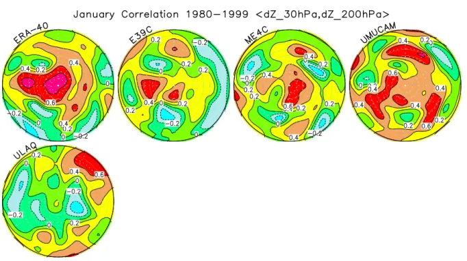
Fig. 1. Correlation between January monthly mean geopotential height anomalies at 200 and 30 hPa during the time period 1980–1999 in the
northern hemisphere. Absolute values larger 0.44 can be considered to be significant at the 95% confidence level. The Greenwich meridian is at 6 o’clock and the southernmost latitude is at 20◦N.
idealised model experiments, but quite often the experimen-tal design is necessarily guided by the needs of assessments and not by our aim to understand the working of our mod-els. Many additional sensitivity studies are often not possible due to time and computational constraints. We are aiming to use existing “scenario”/“typical climate” runs of models and to compare them within a unified statistical framework, diagnosing local correlations/covariances to look at the link between column ozone and meteorology in terms of inter-annual variability on the northern hemisphere during mid-winter. There are two levels of insight we can gain from this exercise: How does the coupling between meteorology and column ozone work in a single model? How do the models and a “proxy of observation” (re-analysis data) compare to each other? What can we learn about the coupling by look-ing at the discrepancies?
The use of monthly mean data, the pre-selection of month (January) and pressure levels (mostly 200 hPa and 30 hPa) used in this analysis are largely guided by the experience gained in the validation and use of the Met Offices Uni-fied Model (UM) with parameterised stratospheric chemistry (UMUCAM, e.g. Braesicke and Pyle, 2003). The 200 hPa level is the lowest upper tropospheric level in which signifi-cant zonal mean changes in ozone and heat flux changes are just detectable in idealised 20 year climate change experi-ments in the UMUCAM (see e.g. Figs. 2b and 6 in Braesicke and Pyle, 2004). In addition Braesicke et al. (2003) estab-lished a robust relation between 200 hPa geopotential heights
and column ozone in UMUCAM and the SLIMCAT CTM column ozone driven by ECMWF analysis for January in the Atlantic/European sector. The impact of vortex strength on high latitude column ozone in UMUCAM during January is strong and is a precondition for spring ozone anomalies in middle latitudes (Braesicke and Pyle, 2003). Even though the initial motivation for choosing the month and levels are largely based on UMUCAM, there is no evidence that this choice disadvantages one of the other participating models. In addition, for the data sets used the separation of the as-sociated Eigenvalues (discriminable and strictly monotonic decreasing between empirical orthogonal functions (EOFs) 1, 2 and 3 in a singular value decomposition sense) is mon-itored to assure the separation, correct order and linear in-dependence of the EOFs. Compared to other winter months this separation is best in January, the month for which we will present our analysis.
A small number of different underlying mechanisms deter-mine the correlation (covariance) patterns between geopoten-tial height anomalies at 200 hPa and column ozone for differ-ent latitude regimes. In middle latitudes we expect a strong modulation of column ozone by the height of the tropopause, which in our case is approximated using geopotential height anomalies at 200 hPa. A high/low tropopause will relate to low/high column ozone and will therefore lead to a nega-tive correlation (e.g. Dobson, 1930; Orsolini et al., 1998 and Steinbrecht et al., 1998). In high latitudes we expect the reverse. Negative/positive geopotential height anomalies
P. Braesicke et al.: Link between column ozone and geopotential height anomalies 2521
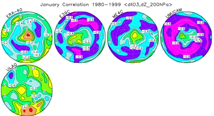
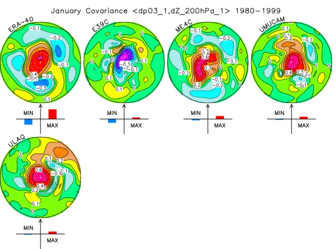
Fig. 2. Correlation between January monthly mean geopotential height anomalies at 200 hPa and monthly mean total column ozone anomalies
during the time period 1980-1999. Absolute values larger 0.44 can be considered to be significant at the 95% confidence level.
at 30 hPa will relate to stronger/weaker vortices which are linked to lower/higher column ozone and thus a positive cor-relation should occur (e.g. Braesicke and Pyle, 2003). This is a combined effect of a suppressed/enhanced meridional cir-culation and a larger/smaller potential of chemical destruc-tion due to lower/higher temperatures. A local high lati-tude impact from dynamics on column ozone is mediated by potential vorticity anomalies (e.g. Ambaum et al. , 2001 and Orsolini and Doblas-Reyes, 2003). For example a posi-tive potential vorticity anomaly (in conjunction with a strong stratospheric vortex) is conjoined with upward bulging isen-tropes, a higher tropopause and lower column ozone. This ef-fect counteracts the previous efef-fect and positive correlations should be weak and small in spatial extent. To test for the link between column ozone and geopotential height anoma-lies we will calculate simple correlation maps first.
To advance our analysis, we have to establish the existence of known and well described leading modes of variability in the model systems analysed. Using northern hemisphere Jan-uary monthly mean anomalies of geopotential height at 200 and 30 hPa and column ozone we derive the leading EOFs and their temporal evolution. EOF1 for geopotential height anomalies is also known as the annular mode and is a well described structure in observations and in some model sys-tems (Baldwin, 2001; Thompson and Wallace, 2001). Near the surface the annular mode shows some distinct asymme-tries relating it to some classical meteorological indices like e.g. the North Atlantic Oscillation (NAO) (Wallace, 2000; Kodera and Kuroda, 2003). Higher up the name “annular
mode” becomes more obvious because of the “very annular” nature of this mode of variability in the stratosphere. EOF2 in geopotential height anomalies in the free troposphere should reveal a tripole structure over the Pacific-North American (PNA) sector, which relates to the so-called PNA pattern (e.g. Wallace and Thompson, 2002) and a wave one struc-ture (one maximum and one minimum in geopotential height anomalies along a longitude line) in the stratosphere. The existence of those spatial structures in the models is a pre-requesit for successfully modelling the link between column ozone and geopotential height anomalies.
There is an ongoing debate about the physical nature of the statistically derived spatial patterns (EOFs) in the free troposphere. Christiansen (2002) argues for their physical nature, based on rotated EOFs at 500 hPa and the fact that positive zonal mean wind anomalies in the stratosphere re-sult in a larger probability for a positive annular mode phase at the surface 30 days later. This is in contrast to Ambaum et al. (2001) where the surface annular mode is described as a product of a mathematical method, and the NAO and PNA pattern are highlighted as the more physical relevant concepts. Even though this situation complicates the under-standing of the physical causes of the differences in charac-teristic spatial patterns, it does not invalidate the attempt to use the patterns in comparing models and to judge them as similar or different.
Subsequently pointwise covariance maps of anomalies as-sociated with EOFs 1 and 2 are calculated; between geopo-tential height anomalies at 200 and 30 hPa and between
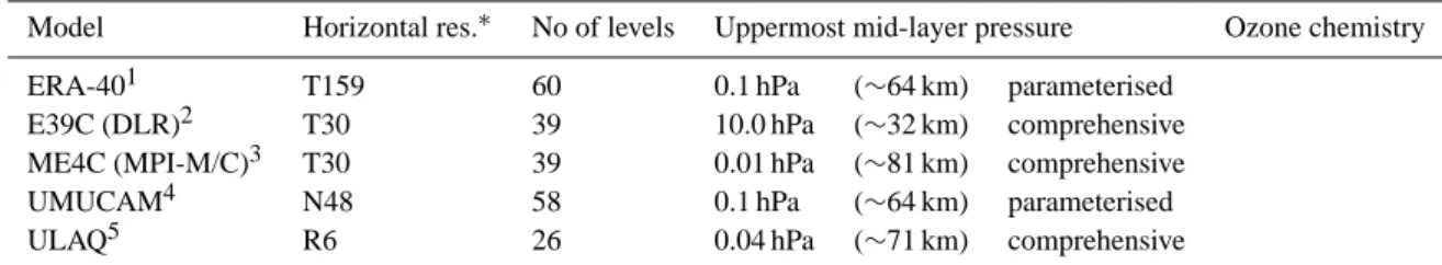
Table 1. Summary of models in this comparison.
Model Horizontal res.∗ No of levels Uppermost mid-layer pressure Ozone chemistry
ERA-401 T159 60 0.1 hPa (∼64 km) parameterised E39C (DLR)2 T30 39 10.0 hPa (∼32 km) comprehensive ME4C (MPI-M/C)3 T30 39 0.01 hPa (∼81 km) comprehensive UMUCAM4 N48 58 0.1 hPa (∼64 km) parameterised ULAQ5 R6 26 0.04 hPa (∼71 km) comprehensive
∗The original spectral (T/R) or regular (N) grid resolution is cited. The analysis grid is N48, see text. 1European Centre for Medium-Range Weather Forecasts (ECMWF) Re-Analysis
2Deutsches Zentrum f¨ur Luft- und Raumfahrt-Institut f¨ur Physik der Atmosph¨are 3Max-Planck-Institut (MPI) f¨ur Meterologie and MPI f¨ur Chemie
4Unified Model University of Cambridge 5Universit`a degli Studi dell’Aquila
geopotential height anomalies at 200 hPa and column ozone anomalies. In conjunction with the corresponding anomaly correlations we will be able to assess the relative strength of the mechanisms discussed above. There are two indicators we will compare:
– The spatial patterns of the scaled hemispheric
covari-ance maps. How similar are the patterns between mod-els and re-analysis data?
– The amplitude (absolute hemispheric maximum minus
minimum) of the covariance patterns derived. How strong is the maximum local coherence/covariance be-tween two levels/quantities?
This will help us to understand which leading modes of vari-ability might be linked, either in terms of height or in terms of different quantities and how the relative importance of lead-ing modes of variability differs in different model systems.
Section 2 details the models and data-sets used in this study and Sect. 3 will provide some more details about the chosen methodology and how it compares to other stud-ies. After establishing the relation described above (Sect. 4) a comparison of characteristic spatial patterns (as approxi-mated by the EOFs 1 and 2) for geopotential height anoma-lies at 200 and 30 hPa and column ozone anomaanoma-lies is pre-sented in Sect. 5. The covariances between reconstructed anomalies between different levels or quantities are dis-cussed in Sect. 6. Section 7 will provide a summary and conclusions.
2 Models and data
For the period considered, 1980–1999, we compare four dif-ferent CCMs and the largely consistent assimilated ERA-40 data-set (Uppala et al., 2005). To some extent we have to consider ERA-40 as a “proxy of observations” because it assimilates meteorology and ozone during the time pe-riod of interest, but there are particularly some limitations
to the assimilation of ozone (Dethof and Holm, 2004). The main ozone constraint is derived from TOMS column mea-surements, therefore a lot of a-priori profile information is maintained and during polar night ozone in high latitudes is not constraint by observations due to a lack of measure-ments. Nevertheless, by the very nature of the assimila-tion scheme used, column ozone (where measured) is nearly identical to TOMS. Problems may arise in high latitudes on the winter hemisphere, when the model relies on the pa-rameterised ozone chemistry alone (a Cariolle scheme, Car-iolle and D´equ´e, 1986) in conjunction with a simple tem-perature dependent parameterisation representing additional ozone loss due to chlorine activation on polar stratospheric clouds). Due to this uncertainty it is not possible to interpret ECMWF fully as an observational data set, but it can be used as a largely well constraint climate model.
The CCM data-sets used in this study are the result of model integrations attempting to represent the time period from 1980–1999 (note that we use a subset of models fea-tured in Eyring et al., 2006). Table 1 presents a brief model summary. As can be seen from the table the range of mod-els is quite diverse (in this context we refer to ERA-40 as a model as well, even though it will be used as an observa-tionsal proxy). To make the intercomparison easier we use a common diagnostic grid for all calculations (note that tests using the original model grids showed no depence of the re-sults on the grid). All model data is interpolated to the N48 grid used by the UMUCAM model, which corresponds to a resolution of 3.75◦in longitude by 2.5◦in latitude on the required pressure levels.
All CCMs we are assessing here treat ozone in the strato-sphere as an interactive trace gas. Some other gases (like CFCs) might be prescribed. The models have either per-formed fully transient runs (E39C, ME4C, ULAQ) or they include a transient component and fix certain other parame-ters to typical 1990s values (UMUCAM). The E39C, ME4C and ULAQ runs have been designed to be as realistic as pos-sible in their representation of the 1980–1999 time period
P. Braesicke et al.: Link between column ozone and geopotential height anomalies 2523
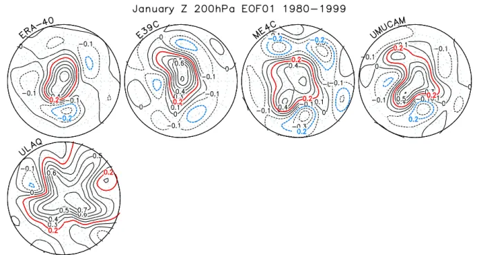
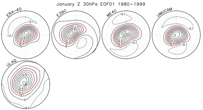
Fig. 3. EOF1 in geopotential height at 200 hPa for January.
using a multitude of specified time varying external forcings. The UMUCAM run was deliberately not designed as a typ-ical scenario integration and uses time varying sea surface temperatures only (other external forcings are set to typi-cal 1990s values) to allow for the easier assessment of se-lected sensitivities. Note that all models prescribe observed monthly mean sea surface temperatures and calculate sur-face pressure, except the ULAQ model, where the sursur-face pressure is fixed to 1000 hPa. This difference is linked to the form of model equations solved, with all models being based on the full set of primitive equations, except the ULAQ model which uses a quasi-geostrophic form of the primitive equations. Details of the models are given in the following papers: E39C (DLR): Dameris et al. (2005, 2006); ME4C (MPI-M/C): Manzini et al. (2003) and Steil et al. (2003); UMUCAM: Braesicke and Pyle (2003, 2004); ULAQ: Pitari et al. (2002). It is interesting to note that most models here are spectral models, solving the equations of motion in wavenumber space. Only UMUCAM is a gridpoint model and does not employ transformations between wavenumber and gridpoint space. In addition, it should be noted that E39C and ME4C are based on the same original model and have mainly deviated by the employed transport scheme and de-velopments of the vertical domain modelled. Here, we assess the interannual variability under the assumption that details of the boundary forcings are not important and that changes in time varying boundary forcings will more stronlgy affect trends. We will return to this assumption later in the conclu-sions.
Table 2. Pattern correlations for geopotential height EOF1 and
EOF2 at 200 hPa. The upper triangle (light gray shading) is for EOF1, the lower triangle (unshaded) is for EOF2. The exact thresh-old for statistical significance is hard to establish, because the cor-rect number of degrees of freedom cannot be established easily. Therefore a subjective highlighting (values above ≥0.5 are in bold) is used as a crude measure of similarity.
Model ERA-40 E39C ME4C UMUCAM ULAQ EOF1 ERA-40 1.0 0.85 0.83 0.89 0.40 ERA-40 E39C 0.26 1.0 0.81 0.83 0.55 E39C ME4C 0.26 0.19 1.0 0.85 0.49 ME4C UMUCAM 0.41 0.66 0.06 1.0 0.65 UMUCAM
ULAQ −0.12 −0.24 −0.19 −0.14 1.0 ULAQ
EOF2 ERA-40 E39C ME4C UMUCAM ULAQ Model
3 Methodology
One simple mechanism for varying column ozone is the change of tropopause heights in middle latitudes (e.g. Dob-son, 1930; Orsolini et al., 1998 and Steinbrecht et al., 1998). The change in tropopause heights is also mirrored in geopo-tential height anomalies at a pressure surface close to the tropopause (e.g. 200 hPa). Even though this effect is most pronounced in middle latitudes, a correlation between col-umn ozone and geopotential height anomalies can be derived anywhere. This concept of “vertical coherence” (e.g. high tropopause/low column ozone or vice versa) can also be ex-tended towards geopotential height anomalies at different pressure levels. Note that this differs from other approaches
looking into interrelations between geopotential heights on pressure levels as e.g. used by Perlwitz et al. (2000).
Note that the methodology does not enable us to find a physical rationale for the characteristic spatial patterns de-rived (e.g. Wallace, 2000; Ambaum et al., 2001; Wallace and Thompson, 2002). We are focusing on the comparison of re-sults between a data assimilation system (as our best guess of observed interannual variability between 1980-1999, with the above mentioned limitations in ozone) and models try-ing to capture the characteristics of interannual variability between 1980 and 1999. Unlike Steinbrecht et al. (2006) we do not attempt the attribution of interannual variability to forcing parameters in a regression model, but we try to unravel the functioning of the coupled variability (between different height regimes) in the models. We assume that si-miliarities in interannual variability will manifest themselves in similar patterns and that deviations from the patterns are linked to deficits or differences in the model systems.
We use monthly mean anomalies of geopotential height and column ozone (in addition we diagnose partial column ozone between 380 and 550 K isentropic temperature levels) and evaluate the relationship between geopotential height and column ozone anomalies by statistical means. As already mentioned in the introduction, we will go through a three step process to assess the links between column ozone and meteorology: First, we will use point-by-point correlations between monthly mean anomalies of geopoptential heights at selected pressure levels and ozone columns to discuss the idea of vertical coherence as explained above. To establish the overall relation of different anomaly time-series, corre-lation coefficients are more intuitive. For the reconstructed anomalies discussed later the standard deviations can be-come regionally very small due to the fixed position of zero lines (given by the characterisitc spatial patterns, EOFs) and therefore correlation coefficients are no longer well defined. Correlations and covariances are related through a scaling with the product of the standard deviations and therefore co-variances are shown. This deliberately simple approach is not limiting the ability to discuss pattern similarities between models, or to pinpoint regions where the concept of local co-herence holds very well or not at all for a given large scale feature. We will make this clear by contrasting our approach with results from literature. Secondly, a detailed investiga-tion of characteristic spatial patterns for the anomaly fields will use the two leading EOFs of geopotential height anoma-lies at different pressure levels and column ozone. We use all anomalies available on the northern hemisphere, unweighted but interpolated to a common horizontal grid (see above). A sensitivity check applying latitudinal weighting left our con-clusions unchanged. Thirdly, a detailed discussion of the point-by-point covariance patterns of reconstructed anoma-lies in geopotential heights and ozone columns using the two leading modes of interannual variability (EOFs 1 and 2) fol-lows. Note that we focus solely on the interannual variability. No assessment of trends (which are removed prior to the
fur-ther analysis) or shifts in climate regimes will be conducted. We assume that the first two EOFs are the same over the time period evaluated (20 years) and assess whether the re-lation between interannual changes in meteorology and col-umn ozone is reproduced in a similar way in the CCMs and the re-analysis data.
4 Anomaly correlations
To illustrate the general behaviour of the models in terms of vertical coherence and their relationship between column ozone and meteorology (as represented by the interannual variation of 200 hPa geopotential height) we will discuss lin-ear correlations between monthly mean anomalies. The cor-relation maps are only used to give us some indication of overall behaviour; they are certainly no measure of cause and effect, but with an underlying idea of how meteorology is linking different levels of the atmosphere and how column ozone is affected by changes in e.g. tropopause height or vor-tex strength (see introduction), we will be able to interpret and compare the resulting patterns.
Figure 1 shows the correlation between January monthly mean geopotential height anomalies at 200 and 30 hPa dur-ing the time period 1980–1999. We know that the interan-nual variability at 30 hPa relates to the characteristics of the winter vortex and there is an amount of coherence between the mid-winter vortex in the stratosphere and the geopoten-tial height anomalies in the upper troposphere. We find rea-sonable agreement between the model data (E39C, ME4C and UMUCAM) and the analysis (ERA-40). All show high positive correlations in high latitudes but the annularity and the absolute amplitude of the patterns are different, with the analysis showing the highest correlations. The ULAQ model shows a very weak signal only in high latitudes with only a small area of positive correlation.
Figure 2 shows the correlation between January monthly mean geopotential height anomalies at 200 hPa and monthly mean column ozone anomalies during the time period 1980– 1999. There are two distinct regimes visible in the correla-tions: a middle latitude one with negative correlation and a polar one with positive correlation. The patterns are more pronounced in the CCMs solving the primitive equations with prescribed boundary forcings than in the analysis or in the ULAQ model (see above). Nevertheless the overall agreement between ERA-40 and E39C, ME4C and UMU-CAM is good.
As mentioned in the introduction, the reason for these two regimes can be understood physically: In middle latitudes column ozone variability on many timescales is to some ex-tent controlled by the tropopause height which is correlated to the height anomaly at 200 hPa. A positive height anomaly (a higher than average tropopause) is related to lower than average column ozone and vice versa leading to a negative correlation. In high latitudes meridional transport and the
P. Braesicke et al.: Link between column ozone and geopotential height anomalies 2525
Fig. 4. EOF1 in geopotential height at 30 hPa for January.
strength of the polar vortex are more important in control-ling the column ozone abundance. A stronger than average vortex (linked to a negative polar height anomaly, see above) is likely to suppress meridional transport and leads therefore to lower polar column ozone and vice versa. This control mechanism is then indicated by a positive correlation pattern in high latitudes (see Sect. 1 for further details).
Using the partial ozone column between 380 and 550 K (most ozone contributing to the total column will be located in this region) instead of the total ozone column does not change the overall behaviour as discussed in conjunction with Fig. 2. A small amount of noise becomes apparent due to the fact that the partial ozone column is derived from pres-sure gridded ozone mixing ratios.
In this section we have confirmed a general picture of the vertical coherence of the models during January on the north-ern hemisphere and a conceptual interpretation of the simple link between column ozone and meteorology (as represented by 200 hPa geopotential height anomalies). In the following we attempt to split this general overall behaviour into com-ponents related to the leading modes of variability in each model system using an EOF analysis.
5 Leading EOFs of heights and column ozone
5.1 EOFs in geopotential heights
As motivated in section 1 we focus on January and discuss the spatial patterns of the EOFs for geopotential height and column ozone anomalies. Thereafter we discuss the spa-tial patterns and amplitudes of covariances calculated using reconstructed anomalies of geopotential height and column ozone for individual leading modes of variability (the focus will be on EOFs 1 and 2 and their associated time evolution and weights).
5.1.1 The vertical structure of the annular mode
We find in the lower free troposphere an annular structure centred over the pole with a marked asymmetry over the Atlantic-West European sector in all models (not shown). The asymmetry is related to the NAO. Schnadt and Dameris (2003) discuss the relationship between the NAO and col-umn ozone recovery in E39C and find a decrease of the NAO index in a future climate in conjunction with a stronger dy-namical heating in the stratosphere. In addition, Braesicke et al. (2003) analyses the NAO signature in column ozone for two different models, including UMUCAM. There is an-other asymmetry in most models (including ERA-40) to-wards the Pacific sector. This asymmetry is most pronounced in ME4C. The asymmetries are generally weak in the ULAQ model, presumably related to the fixed surface pressure and the lower horizontal resolution.
Figure 3 shows EOF1 in geopotential height at 200 hPa for January. The polar annular structure is already smoother
compared to further down but pronounced asymmetries can be seen. The one identified in the Atlantic-West European sector is still apparent and there is a pronounced anomaly in the Pacific-Asian sector. The CCMs with a resolution above or equal to T30 compare well with the ERA-40 anomalies.
Figure 4 shows EOF1 in geopotential height at 30 hPa for January. The two models with a higher upper boundary and higher horizontal resolution (ME4C and UMUCAM) show two distinct minima in middle latitudes, whereas only one minimum is seen in ERA-40. In general this plot reveals the climatological position of the polar vortex during Januray in the models. Note that all troposphere-resolving CCMs show a clear shift of the polar vortex towards the Atlantic/West Eu-ropean sector, but E39C shows a displacement of the annular mode pattern towards the North American sector.
The models with variable surface pressure (E39C, ME4C and UMUCAM) show a good comparison with observations (ERA-40). The model with a fixed surface pressure (ULAQ) has some problems with the tropospheric annular mode and the NAO related asymmetries, but does perform well in the stratosphere.
5.1.2 EOF2 at selected pressure heights
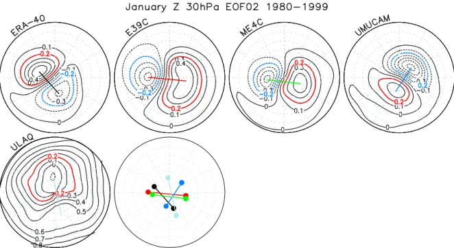
Figure 5 shows EOF2 in geopotential height at 200 hPa for January. Much more small scale stucture is obvious as com-pared to EOF1. A prominent feature is a tripole over the Pacific-North American sector, which relates to the so-called PNA pattern (e.g. Wallace and Thompson, 2002). Wal-lace and Thompson (2002) discussed this pattern in their Fig. 4, derived by regressing the second principal component (PC2) of surface level pressure anomalies onto geopotential height anomalies at 500 hPa. Because we focus on geopoten-tial height changes and their local impact on column ozone amounts, we focus on lower pressures (larger altitudes) com-pared to Christiansen (2002) (see Sect. 1) to better approx-imate local tropopause changes. In addition our data base is sparser (monthly mean data compared to daily 30-day low pass filtered) and we therefore focus clearly on the interan-nual timescale and not on smoothly and continuously varying data. Given the nature of our data and the chosen pressure surface we do not require a rotation of the EOFs to reveal the PNA pattern. To highlight the relative position of the PNA patterns in each model the strongest maxima relating to the tripole structure are marked out with connecting lines, which are repeated on a common map in Fig. 5. The agreement between ME4C and UMUCAM is quite striking, given that they are very different models in terms of their model formu-lation (spectral versus gridpoint, different choice of prognos-tic variables, etc.). E39C displays a slightly more elongated tripole structure reaching more into the Atlantic sector (see comparison of positions of extrema in the lower right part of Fig. 5). In addition to the tripole/PNA structure ERA-40 also indicates a second tripole structur in the Atlantic-European sector which cannot be so readily identified in E39C, ME4C
P. Braesicke et al.: Link between column ozone and geopotential height anomalies 2527
Fig. 6. EOF2 in geopotential height at 30 hPa for January and position markers for the minimum and maximum of EOF2 (repeated in the
lower right plot).
and the UMUCAM model. The ULAQ model also shows smaller scale features in EOF2, but the position of the fea-tures do not relate well to the observations or other CCMs.
As illustrated in Table 2, area weighted spatial correlations for a simple (more annular) spatial structure like EOF1 are generally high between the models. In contrast, the correla-tions for EOF2 are generally much smaller, with UMUCAM and E39C being the most similar. Even though the agreement in the North American/Pacific sector is very good between ME4C and UMUCAM, the correlation is brought down by the out-of-phase (but low amplitude) behaviour in other sec-tors. Note also that the wavetrain for the ULAQ model is very different from ERA-40 and correlations are therefore weakly negative.
Figure 6 shows EOF2 in geopotential height at 30 hPa for January. All models show a strong “wavenumber 1” struc-ture (one minimum and one maximum along a longitude line), apart from the ULAQ model where the “wavenumber 1” structure is only unincisive. The phase of the anoma-lies (position of the absolute minimum and maximum, see the lower right plot in Fig. 6) differ substantially between all CCMs and ERA-40, with E39C and ME4C displaying some agreement.
5.2 EOFs in total and partial column ozone
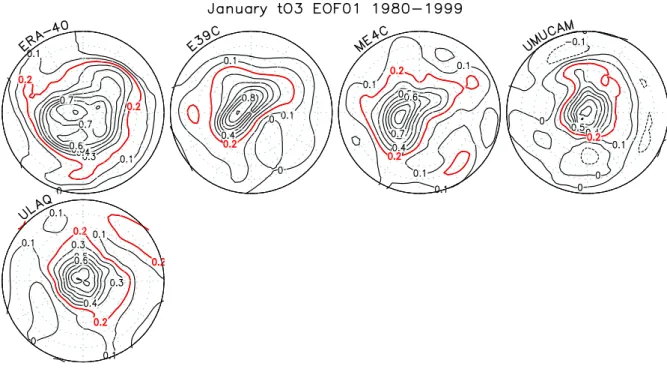
Figure 7 shows EOF1 in column ozone for January. Note, that even though the ERA-40 column ozone data in lower lat-itudes is constrained by the assimilation of column ozone ob-served from the TOMS instrument that constraint is not
avail-able during polar night in high latitudes where the TOMS in-strument cannot measure due to the unavailability of light (see detail above about the parameterised ozone scheme used). EOF1 in column ozone as provided by the ERA-40 data shows a very wide annular mode with a strongly con-fined outer gradient region. This feature might be partially due to the assimilation system, switching over from an area with TOMS data to an area without TOMS data assimila-tion. All models do have an annular mode structure in col-umn ozone as well, but slightly more confined towards polar latitudes. E39C and ME4C do show a more elongated pattern than the UMUCAM and ULAQ models.
EOF1 in partial column ozone (380–550 K) for January (not shown) compares well to Fig. 7 showing column ozone. The ERA-40 pattern appears to widen and an elongated core region appears. Interestingly, in E39C and ME4C the annu-lar pattern shrinks and the elongation of the dominant pat-tern is more apparent, whereas the UMUCAM and ULAQ models are still fairly annular. Certainly those features de-pend crucially on the modelled ozone profiles and their rel-ative positions with respect to the isentropic levels chosen. There is some kind of family similarity between the E39C and ME4C models, both using the same dynamical core and similar chemistry, implying that the result depends more on the troposphere and is not influenced by the different choice of upper boundaries. Interestingly, the UMUCAM model with complex dynamics but simple chemistry and the ULAQ model with simple dynamics and complex chemistry show a similar more annular pattern compared to E39C and ME4C. The ERA-40 result is difficult to interpret; the pattern widens
Fig. 7. EOF1 in total ozone for January.
P. Braesicke et al.: Link between column ozone and geopotential height anomalies 2529
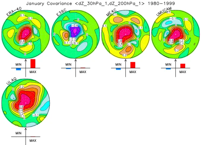
Fig. 9. Covariance of reconstructed geopotential height anomalies at 30 (EOF1) and 200 hPa (EOF1) for January.
and even though it does show some elongation the pattern is less well defined and shows a different orientation to E39C and ME4C results. In addition, the pattern reaches far out into low latitudes, which is not seen in any of the models. As mentioned earlier, this behaviour may be caused in part by the assumptions made in the data assimilation scheme on how to distribute the measured TOMS column ozone data vertically. Note that these differences have not affected the correlations between geopotential height and (partial) col-umn ozone anomalies as discussed in Sect. 4.
Figure 8 shows EOF2 in column ozone for January. ERA-40 and the ULAQ model seem to show some compensation pattern with respect to EOF1 which is still fairly annular, whereas E39C and ME4C show a well defined dipole struc-ture with a very similar orientation. The UMUCAM model indicates a tripole structure leading from North America over the Pacific towards Russia.
EOF2 in partial column ozone for January (not shown) re-veals a largely similar behaviour compared to the column ozone. E39C still shows a clear dipole structure whereas ME4C now indicates a tripole structure reaching from the American sector towards the Atlantic-West European sector. A very similar pattern is found in the UMUCAM model with
a weaker second tripole adjacent to the dominant one. For EOF1 in column ozone the four CCMs are similar. All show a fairly annular mode confined to polar latitudes. In-terestingly, ERA-40 indicates a much wider annular mode. For the partial column ozone the ERA-40 structure widens even more, but the models are now clearly in two groups, either showing a confined elongated pattern (E39C, ME4C) or a more annular behaviour (UMUCAM, ULAQ). The be-haviour for EOF2 is less conclusive and more varied.
6 Covariances for reconstructed anomalies
A simple measure of vertical coherence as explained in Sect. 3 is explored. The covariance between two reconstructed time series (as given by the product of EOF (spatial), princi-pal component (PC, temporal) and weight) is calculated and presented as a map. In addition, we compare this approach to coupled mode analysis available in the literature. To provide the important information in a compact form we will only show maps for EOF1-EOF1 covariances; the other possible combinations are summarised in bar charts showing ampli-tudes only.
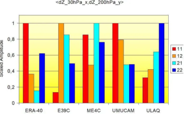
Fig. 10. Amplitudes of geopotential height covariance patterns scaled with the maximum amplitude found in each model.
6.1 Covariances for height anomalies at different pressures Figure 9 shows the covariance of reconstructed geopotential height anomalies at 30 (EOF1) and 200 hPa (EOF1) for Jan-uary. As expected from the straightforward covariance ap-proach discussed earlier we find a polar annular region of positive covariance in ERA-40 with a significant amplitude. This feature is also seen in ME4C and the UMUCAM model (both resolving the stratosphere), but with a slightly weaker amplitude. The ULAQ model indicates a larger area of pos-itive covariance but with no significant amplitude, whereas E39C shows a small polar region of negative covariance sur-rounded by small areas of positive correlations but similar to the ULAQ model the amplitude is very low. All models including a comprehensive stratosphere show a positive co-herence/covariance between the 30 and 200 hPa levels (but with the ULAQ model not showing a significant amplitude). E39C with a low upper lid displays a pattern of opposite sign but shows also a very low amplitude, hinting towards a very weak coherence.
Figure 10 compares the relative amplitude distribution for the covariance patterns in each model system. Note that the bars are now scaled against the maximum amplitude found in each individual model. The numbers in the legend to the right refer to the x and y place holders in the bar graph title, identifying the pair of EOFs used to calculate the covariance amplitudes with respect to the earlier figures. ERA-40 shows the largest amplitudes for covariance patterns calculated with the same order (e.g. EOF1-EOF1 (11) or EOF2-EOF2 (22)) at the two different heights considered. This is in good agree-ment with Perlwitz and Graf (1995) and their description of two coupled natural modes during NH winter, one describ-ing the link between stratospheric vortex strength and tro-pospheric circulation over the North Atlantic (11) (this link has been recently re-examined by Walter and Graf, 2005 and Graf and Walter, 2005) and the other linking the stratospheric zonal wavenumber 1 with a PNA-like pattern in the strato-sphere (22). None of the models reproduce this clear
sepa-ration in the amplitude distribution. E39C has strongest am-plitudes for the mixed modes (12) and (21). This is less ob-vious in ME4C which shows a stronger (11) covariance am-plitude. UMUCAM shows the strongest amplitude for (11) as in ERA-40, but drops of towards higher orders, whereas ULAQ shows the converse behaviour.
In general, most models display a reasonable amount of vertical coupling (e.g. a significant amplitude in the covari-ance), with the ULAQ model showing the weakest vertical coherence. E39C tends towards coupling involving higher tropospheric EOFs (EOF1-EOF2 coupling) to reproduce the overall positive correlation in polar latitudes between tro-pospheric and stratospheric polar height anomalies, whereas ME4C and the UMUCAM model both show a clear EOF1-EOF1 coupling.
6.2 Covariances for column ozone and height anomalies Here, we will evaluate the relationship between (partial) col-umn ozone anomalies and geopotential height anomalies at 200 hPa.
Figure 11 shows the covariance of reconstructed geopoten-tial height anomalies at 200 hPa (EOF1) and pargeopoten-tial column ozone anomalies (EOF1) for January. Even though the par-tial column ozone EOF1 derived from ERA-40 data is wide, a well defined annular region of positive covariance in polar latitudes surrounded by some smaller negative anomalies is apparent. The shape of the anomalies in the CCMs is largely determined by the column ozone EOF1 pattern. The covari-ances are fairly annular for UMUCAM and ULAQ and elon-gated for E39C and ME4C. The phase problem identified ear-lier in the geopotential height analysis is now apparent again in the E39C results. Note that all CCMs have a much smaller amplitude than ERA-40. The weak negative covariances in low latitudes seem to support the idea that the meridional motion in conjunction with the vortex strength (EOF1 for geopotential heights should be a good proxy of the overall vortex strength, see descussion of annular modes above) is regulating high latitude ozone on interannual timescales, but does not hugely affect lower latitudes where “tropospheric weather” (tropopause height as e.g. approximated by 200 hPa geopotential height anomalies) is more important. This mod-ulation of the poleward meridional transport might be less well represented in E39C due to the lower upper boundary. This is also in agreement with Braesicke and Pyle (2003), in which the best proxy for the UMUCAM vortex strength with respect to column ozone in high latitudes was identfied as the 60◦N, 10 hPa zonal-mean zonal wind, indicating that transport processes in and around this level are important to maintain the correlation.
Figure 12 compares the relative amplitude distribution for the covariance patterns in each model system. It is organised like Fig. 10, but shows the covariance amplitudes for partial ozone columns and geopotential heights at 200 hPa. ERA-40 shows the largest amplitude for the covariance pattern
calcu-P. Braesicke et al.: Link between column ozone and geopotential height anomalies 2531
Fig. 11. Covariance of reconstructed geopotential height anomalies at 200 hPa (EOF1) and partial column ozone anomalies (EOF1) for
January.
lated with the leading order (EOF1-EOF1) at the two differ-ent variables with a continuous drop in amplitude to higher orders. This behaviour is not reproduced in the other mod-els. They show generally higher amplitudes for higher order covariances, within the amplitude range modelled by each model.
A particularly interesting example is the amplitude calcu-lated for EOF2s in geopotential heights and column ozone. Orsolini (2004) describes seesaw fluctuations of column ozone related to North Pacific and North Atlantic surface pressure differences during February and compares those to the AO modulation of column ozone. The Aleutian-Icelandic Index (AII) (as discussed in e.g. Honda and Nakamura (2001)) used in this paper correlates highly with the PNA pattern and the AII regressed column ozone shows more pro-nounced out-of-phase extremas over both, the North Pacific and North Atlantic, compared to an surface annular mode regressed February column ozone map. The covariance for column ozone (EOF2) and geopotential height anomalies at 200 hPa (EOF2) (Fig. 13) reveal pronounced maxima over the Pacific sector for ERA-40, ME4C and UMUCAM. The pattern is similar to the one revealed by the AII regression on
Fig. 12. Amplitudes of ozone/geopotential height covariance
pat-terns scaled with the maximum amplitude found in each model sys-tem.
Fig. 13. Covariance of reconstructed geopotential height anomalies at 200 hPa (EOF2) and partial column ozone anomalies (EOF2) for
January.
column ozone for February (Fig. 5 in Orsolini, 2004). The hemispheric agreement between ERA-40 and ME4C is best, with more small scale structures visible in UMUCAM Even though E39C has a strong signal the extrema are very close to the pole.
The agreement between CCMs with higher horizontal res-olution and ERA-40 data is generally good with respect to the overall pattern, even though there are differences in the relative amplitude of the pattern. The model with the lowest upper lid (E39C) displays a preference for the tropospheric EOF2 being more important compared to ME4C and the UMUCAM model. The ULAQ model agrees well for EOF1-EOF1 covariances only and shows, in all cases discussed, the weakest amplitude.
The agreement between CCMs with higher horizontal res-olution and ERA-40 data is generally good with respect to the overall pattern, even though there are differences in the relative amplitude of the pattern. The model with the lowest upper lid (E39C) displays a preference for the tropospheric EOF2 being more important compared to ME4C and the UMUCAM model. The ULAQ model agrees well for EOF1-EOF1 covariances only and shows, in all cases discussed, the weakest amplitude.
6.3 Vertical polar temperature profiles
The importance of the vertical descretization in numerical models of the atmosphere has been discussed extensively (e.g. Simmons and Burridge, 1981. In addition, care has to be taken in selecting the right upper boundary condition (in-cluding the spacing of the vertical levels and damping mech-anisms) to avoid arbitrary reflection of vertically propagating waves. A simple measure for buoyancy controlled waves is the vertical temperature gradient. It provides some insight in how the vertical layering of the model and the chosen upper boundary condition affect the (thermo-)dynamic structure of a model.
Figure 14 shows January polar mean temperature profiles averaged over 70◦N northward (left) and corresponding ver-tical temperature gradients (right) for all four CCMs and ERA-40. Note that the area for the averaging is somehow ar-bitrarily chosen. The following discussion will only attempt to illustrate the points made above in terms of two very basic quantities: an averaged temperature profile and the associ-ated vertical gradient. There are three points to note:
– The UMUCAM model is the coldest in the middle
P. Braesicke et al.: Link between column ozone and geopotential height anomalies 2533 190 195 200 205 210 215 220 Temperature [K] 8 12 16 20 24 28 32 Altitude [km] ERA-40 E39C ME4C UMUCAM ULAQ -5 -4 -3 -2 -1 0 1 2 dT/dz [K/km] 8 12 16 20 24 28 32 30hPa 200hPa
Fig. 14. Left: January polar mean temperature profiles averaged
over 70. N northward. Right: Vertical temperature gradients de-rived from interpolated temperature profiles (dashed lines, left).
lowermost stratosphere, where ULAQ and UMUCAM are reasonably matched to ERA-40.
– The vertical temperature gradient reverses in E39C
above 26 km. This feature is quite certainly related to the lower upper boundary and seems to be con-sistent with the stronger impact of tropospheric lower wavenumbers/higher order EOFs as revealed by the above analysis.
– Even though the ULAQ model matches the
tempera-tures in the stratosphere well compared to ERA-40, it has a less pronounced tropospheric local maximum in the temperature gradient.
Even though this is a very simple diagnostic and not indepen-dent from the flowfield and the resolution of the models, the results are consistent with the overall behaviour of the mod-els as shown by the covariance analysis. It is encouraging to note that all troposphere resolving CCMs with a strato-sphere do show some similarities in the coupled interannual variability of column ozone and geopotential heights.
7 Summary, conclusions and outlook
We applied a statistical analysis framework to analyse some aspects of the combined interannual variability of north-ern hemisphere column ozone and meteorology during mid-winter (January) in four CCMs and in ERA-40.
We confirmed a general picture of the vertical coherence of the models during January on the northern hemisphere and a conceptual interpretation for a simple link between column ozone and meteorology (as represented by 200 hPa geopoten-tial height anomalies) during January, discussing the com-bined effect of meridional transport towards high latitudes,
vortex strength and variations in tropause height in middle latitudes.
The statistical significance of many of our results is low, not withstanding the fact that some quantities will show significant differences on a decadal timescales in idealised model simulations (Braesicke and Pyle, 2003). Neverthe-less, it is encouraging that understanding, based on physi-cal processes, is consistent with many aspects of the correla-tion/covariance structures which we diagnose.
For the spatial patterns of the geopotential height EOF1 at different pressure levels (the annular mode) we find good agreement between the models with variable surface pres-sure (E39C, ME4C and UMUCAM) and the re-analysis data (ERA-40). The model with a fixed surface pressure (ULAQ) has some problems with the tropospheric annular mode and the NAO related asymmetries, but does perform reasonably well in the lower stratosphere. Note that a recent study by Stenchikov et al. (2006) analysed the Arctic Oscillation (AO) response to volcanic eruptions as simulated by IPPC AR4 models and found a general underestimation of the AO vari-ability, which is in general agreement with the low CCM amplitudes of the EOF1-EOF1 covariances between 30 and 200 hPa (not shown).
Most models in this study display a reasonable amount of vertical coupling (e.g. a significant amplitude in the co-variance) in their geopotential height anomalies, with the ULAQ model showing the weakest vertical coherence. E39C seems to prefer a coupling involving higher tropospheric EOFs (EOF1-EOF2 coupling) to reproduce the overall pos-itive correlation in polar latitudes between tropospheric and stratospheric polar height anomalies, whereas ME4C and the UMUCAM model both show a clear EOF1-EOF1 coupling.
For the covariances between column ozone and geopoten-tial height anomalies at 200 hPa we find good agreement be-tween the CCMs with higher horizontal resolution and ERA-40 data with respect to the overall pattern, even though there are differences in the relative amplitudes of the pattern. The model with the lowest upper lid (E39C) displays again a preference for the tropospheric EOF2 being more important compared to ME4C and the UMUCAM model. The ULAQ model agrees well for the EOF1-EOF1 covariance only and shows in all cases discussed the weakest amplitude.
The PNA pattern emerges as a useful qualitative bench-mark for the model performance. Models with higher hor-izontal resolution and high upper boundary (ME4C and UMUCAM) show good agreement with the PNA tripole de-rived from ERA-40 data, including the column ozone modu-lation over the Pacific sector. The model with lowest horizon-tal resolution does not show a classic PNA pattern (ULAQ), and the model with the lowest upper boundary (E39C) does not capture the PNA related column ozone variations over the Pacific sector.
The above has implications for the use of CCMs in cli-mate predictions. The findings presented here should be kept in mind when analysing model simulations for the near and
far future. As long as we are sure that the modes of vari-ability stay similar under climate change (as prescribed by chosen boundary conditions) the troposphere resolving mod-els should perform well (the assumption about similar modes is only save for the near future, assuming that we are not to close to a critical threshold). Note that other model assump-tions may need adjusting, e.g. the parameterised ozone chem-istry in UMUCAM (depending on the application). Simpler models need to restrict their interpretation of future climate to sensitivity studies.
Future work will also focus on the spring season, analysing the ability of models to simulate the dynamical control of ozone during and after the stratospheric vortex break-up in middle latitudes on the northern hemisphere (e.g. Orsolini and Doblas-Reyes, 2003) and the same methodology can be used to assess climate change integrations.
Acknowledgements. The authors would like to acknowledge the
support of the EU integrated project SCOUT-O3. In addition, P. Braesicke and J. A. Pyle would like to thank NERC for support through NCAS. We would like to thank two anonymous reviewers for their supportive and constructive comments.
Edited by: W. T. Sturges
References
Ambaum, M. H. P., Hoskins, B. J., and Stephenson, D. B.: Arc-tic oscillation or North AtlanArc-tic oscillation?, J. Climate, 14(16), 3495–3507, 2001.
Baldwin, M. P.: Annular modes in global daily surface pressure, Geophys. Res. Lett., 28, 4115–4118, 2001.
Baldwin, M. P. and Dunkerton, T. J.: Propagation of the Arctic Os-cillation from the stratosphere to the troposphere, J. Geophys. Res.-Atmos., 104(D24), 30 937–30 946, 1999.
Braesicke, P., Jrrar, A., Hadjinicolaou, P., and Pyle, J. A.: Variabil-ity of total ozone due to the NAO as represented in two different model systems, Met. Z., 12, 203–208, 2003.
Braesicke, P. and Pyle, J. A.: Changing ozone and changing circu-lation in northern mid-latitudes: Possible feedbacks?, Geophys. Res. Lett., 30, 1059, doi:10.1029/2002GL015973, 2003. Braesicke, P. and Pyle, J. A.: Sensitivity of dynamics and ozone to
different representations of SSTs in the Unified Model, Q. J. R. Meteorol. Soc., 130, 2033–2045, 2004.
Cariolle, D. and D´equ´e, M.: Southern hemisphere medium-scale waves and total ozone disturbances in a spectral general circula-tion model, J. Geophys. Res., 91, 10 825–10 846, 1986. Christiansen, B.: On the physical nature of the Arctic Oscillation,
Geophys. Res. Lett., 29(16), doi:10.1029/2002GL015208, 2002. Cohen, J. and Saito K.: A test for annular modes, J. Climate, 15(17),
2537–2546, 2002.
Dameris, M., Grewe, V., Ponater, M., Deckert, R., Eyring, V., Mager, F., Matthes, S., Schnadt, C., Stenke, A., Steil, B., Br¨uhl, C., and Giorgetta, M. A.: Long-term changes and variability in a transient simulation with a chemistry-climate model employing realistic forcing, Atmos. Chem. Phys., 5, 2121–2145, 2005, http://www.atmos-chem-phys.net/5/2121/2005/.
Dameris, M., Matthes, S., Deckert, R., Grewe, V., and Ponater, M.: Solar cycle effect delays onset of ozone recovery, Geophys. Res. Lett., 33, L03806, doi:10.1029/2005GL024741, 2006.
Dethof, A. and Holm, E. V.: Ozone assimilation in the ERA-40 reanalysis project, Q. J. Roy. Meteorol. Soc., 130, 2851–2872, 2004.
Dobson, G. M. B.: Observations of the amount of ozone in the Earth’s atmosphere and its relations to other geophysical con-ditions, Proc. Soc. London Ser. A, 129, 411–433, 1930. Eyring, V., Harris, N. R. P., Rex, M., et al.: A strategy for
process-oriented validation of coupled chemistry-climate models, Bull. Am. Meteorol. Soc., 86(8), 1117–1133, 2005.
Eyring, V., Butchart, N., Waugh, D. W., et al.: Assessment of temperature, trace species, and ozone in chemistry-climate model simulations of the recent past, J. Geophys. Res., D22308, doi:10.1029/2006JD007327, 2006.
Graf, H.F., and K. Walter: Polar vortex controls coupling of North Atlantic Ocean and Atmosphere, Geophys. Res. Lett., 32(1), L01704, doi:10.1029/2004GL020664, 2005.
Honda, M., and Nakamura, H.: Interannual seesaw between the Aleutian and Icelandic lows. Part II: Its significance in the in-terannual variability over the wintertime Northern Hemisphere, Journal of Climate, 14(24), 4512–4529, 2001.
Kodera, K. and Kuroda, Y.: Regional and hemispheric circulation patterns in the northern hemisphere winter, or the NAO and the AO, Geophys. Res. Lett., 30, 1934, doi:10.1029/2003GL017290, 2003.
Manzini, E., Steil, B., Br¨uhl, C., Giorgetta, M. A., and Kr¨uger, K.: A new interactive chemistry-climate model. 2. Sensitivity of the middle atmosphere to ozone depletion and increase in greenhouse gases: Implications for recent stratospheric cooling, J. Geophys. Res., 108, 4429, doi:10.1029/2002JD002977, 2003. Orsolini, Y.J.: Seesaw fluctuations in ozone between the North Pa-cific and North Atlantic, J. Met. Soc. Japan, 82(3), 941–949, 2004.
Orsolini, Y. J., Stephenson, D. B., and Doblas-Reyes, F. J.: Storm track signature in total ozone during northern hemisphere winter, Geophys. Res. Lett., 25, 2413–2416, 1998.
Orsolini, Y. J. and Doblas-Reyes, F. J.: Ozone signatures of climate patterns over the Euro-Atlantic sector in the spring, Q. J. R. Me-teorol. Soc., 129, 3251–3263, 2003.
Perlwitz, J. and Graf, H. F.: The statistical connection be-tween tropospheric and stratospheric circulation of the northern-hemisphere in winter, J. Climate, 8(10), 2281–2295, 1995. Perlwitz, J., Graf, H. F., and Voss, R.: The leading variability mode
of the coupled troposphere-stratosphere winter circulation in dif-ferent climate regimes, J. Geophys. Res.-Atmos. 105(D5), 6915-6926, 2000.
Pitari, G., Mancini, E., Rizi, V., and Shindell, D. T.: Impact of fu-ture climate and emission changes on stratospheric aerosols and ozone, J. Atmos. Sci., 59, 414–440, 2002.
Pyle, J. A., Braesicke, P., and Zeng, G.: Dynamical variability in the modelling of chemistry-climate interactions – Faraday Discuss., 130, 27–39, doi:10.1039/b417947c, 2005.
Randel, W., Udelhofen, P., Fleming, E., et al.: The SPARC in-tercomparison of middle-atmosphere climatologies, J. Climate, 17(5), 986–1003, 2004.
Rex M., Salawitch R. J., von der Gathen P., Harris N. R. P., Chip-perfield M. P., and Naujokat B.: Arctic ozone loss and climate
P. Braesicke et al.: Link between column ozone and geopotential height anomalies 2535
change, Geophys. Res. Lett., 31, L04116, 2004.
Schnadt, C. and Dameris, M.: Relationship between NAO changes and stratospheric ozone recovery in the northern hemi-sphere in a chemistry-climate model, Geophys. Res. Lett., 30, doi:10.1029/2003GL017006, 2003.
Simmons, A. J. and Buridge, D.M.: An energy and angular-momentum conserving vertical finite-difference scheme and hy-brid vertical-coordinate, Monthly Weather Review, 109(4), 758– 766, 1981.
Steil, B., Br¨uhl, C., Manzini, E., Crutzen, P. J., Lelieveld, J., Rasch, P. J., Roeckner, E., and Kr¨uger, K.: A new interactive chemistry-climate model. 1. Present day climatology and inter-annual variability of the middle atmosphere using the model and 9 years of HALOE/UARS data, J. Geophys. Res., 108, 4290, doi:10.1029/2002JD002971, 2003.
Steinbrecht, W., Claude, H., Kohler, U., et al.: Correlations between tropopause height and total ozone: Implications for long-term changes, J. Geophys. Res.-Atmos., 103, 19 183–19 192, 1998. Steinbrecht, W., Haßler, B., Br¨uhl, C., Dameris, M., Giorgetta, M.
A., Grewe, V., Manzini, E., Matthes, S., Schnadt, C., Steil, B., and Winkler, P.: Interannual variation patterns of total ozone and lower stratospheric temperature in observations and model sim-ulations, Atmos. Chem. Phys., 6, 349–374, 2006,
http://www.atmos-chem-phys.net/6/349/2006/.
Stenchikov, G., Hamilton, K., Stouffer, R. J., Robock, A., Ramaswamy, V., Santer, B., and Graf, H.-F.: Arctic Os-cillation response to volcanic eruptions in IPCC AR4 cli-mate models, J. Geophys. Res.-Atmos., 111(D7), D07107, doi:10.1029/2005JD006286, 2006.
Thompson, D. W. J. and Wallace, J. M.: The Arctic Oscillation signature in the wintertime geopotential height and temperature fields, Geophy Res. Lett., 25, 1297–1300, 1998.
Thompson, D. W. J., Baldwin, M. P., and Wallace, J. M.: Strato-spheric connection to Northern Hemisphere wintertime weather: Implications for prediction, J. Climate, 15(12), 1421–1428, 2002.
Uppala, S. M., Kallberg, P. W., Simmons, A. J., et al.: The ERA-40 re-analysis, Q. J. R. Meteorol. Soc., 131, 2961–3012, 2005. Wallace, J. M. and Gutzler, D. S.: Teleconnections in the
geopoten-tial height field during the northern hemisphere winter, Monthly Weather Rev., 109(4), 784–812, 1981.
Wallace, J. M.: North Atlantic Oscillation/annular mode: Two paradigms – one phenomenon, Q. J. R. Meteorol. Soc., 126, 791– 805, 2000.
Wallace, J. M. and Thompson, D. W. J.: The Pacific center of action of the northern hemisphere annular mode: Real or artifact?, J. Climate, 15, 1987–1991, 2002.
Walter, K. and Graf, H. F.: The North Atlantic variability struc-ture, storm tracks, and precipitation depending on the polar vor-tex strength, Atmos. Chem. Phys., 4, 6127–6148, 2005, http://www.atmos-chem-phys.net/4/6127/2005/.