Sensitivity analysis by the adjoint chemistry transport model DRAISfor an episode in the Berlin Ozone (BERLIOZ) experiment

HAL Id: hal-00295941

https://hal.archives-ouvertes.fr/hal-00295941

Submitted on 20 Jun 2006

HAL is a multi-disciplinary open access

archive for the deposit and dissemination of

sci-entific research documents, whether they are

pub-lished or not. The documents may come from

teaching and research institutions in France or

abroad, or from public or private research centers.

L’archive ouverte pluridisciplinaire HAL, est

destinée au dépôt et à la diffusion de documents

scientifiques de niveau recherche, publiés ou non,

émanant des établissements d’enseignement et de

recherche français ou étrangers, des laboratoires

publics ou privés.

model DRAISfor an episode in the Berlin Ozone

(BERLIOZ) experiment

K. Nester, H.-J. Panitz

To cite this version:

K. Nester, H.-J. Panitz. Sensitivity analysis by the adjoint chemistry transport model DRAISfor an

episode in the Berlin Ozone (BERLIOZ) experiment. Atmospheric Chemistry and Physics, European

Geosciences Union, 2006, 6 (8), pp.2091-2106. �hal-00295941�

www.atmos-chem-phys.net/6/2091/2006/ © Author(s) 2006. This work is licensed under a Creative Commons License.

Chemistry

and Physics

Sensitivity analysis by the adjoint chemistry transport model

DRAIS for an episode in the Berlin Ozone (BERLIOZ) experiment

Institut f¨ur Meteorologie und Klimaforschung (IMK), Forschungszentrum Karlsruhe/Universit¨at Karlsruhe, Hermann-von-Helmholtz-Platz 1, 76344 Eggenstein-Leopoldshafen, Germany

Received: 2 May 2005 – Published in Atmos. Chem. Phys. Discuss.: 13 September 2005 Revised: 16 January 2006 – Accepted: 19 April 2006 – Published: 20 June 2006

Abstract. The Berlin Ozone Experiment (BERLIOZ) was carried out in summer 1998. One of its purposes was the evaluation of Chemistry Transport Models (CTM). CTM

KAMM/DRAIS was one of the models considered. The

data of 20 July were selected for evaluation. On that day, a pronounced ozone plume developed downwind of the city. Evaluation showed that the KAMM/DRAIS model is able to reproduce the meteorological and ozone data observed, ex-cept at farther distances (60–80 km) downwind of the city. In that region, the DRAIS model underestimates the measured ozone concentrations by 10–15 ppb, approximately.

Therefore, this study was conducted to detect possible rea-sons for this deviation. A comprehensive sensitivity analysis was carried out to determine the most relevant model param-eters. The adjoint DRAIS model was developed for this pur-pose, because for this study the application of this model is the most effective method of calculating the sensitivities. The least squares of the measured and simulated ozone concen-trations between 08:00 UTC and 16:00 UTC at two stations 30 km and 70 km downwind of the city centre were chosen as distance function. The model parameters considered in this study are the complete set of initial and boundary species concentrations, emissions, and reaction rates, respectively. A sensitivity ranking showing the relevance of the individ-ual parameters in the set is determined for each parameter set.

In order to find out which modification in the parameter sets most reduces the cost function, simplified 4-D data as-similation was carried out. The result of this data assimila-tion shows that modificaassimila-tions of the reacassimila-tion rates provide the best agreement between the measured and the simulated ozone concentrations at both stations. However, the modified reaction rates seem to be unrealistic for the whole simulation period. Therefore, the good agreement should not be

overes-Correspondence to: H.-J. Panitz

([email protected])

timated. The agreement is still acceptable when the parame-ters in the other sets are modified together. The investigation demonstrates that an analysis of this type can help to explain inconsistencies between observations and simulations. But in the case considered here the inconsistencies cannot be ex-plained by an error in only one parameter set.

1 Introduction

The Berlin Ozone (BERLIOZ) Experiment (Becker et al., 1999) was carried out in the period between 13 July and 9 August 1998, as part of the German Tropospheric Research Programme (TSF). The experimental domain comprised the city of Berlin and an area within a radius of about 100 km around the city. The experiment mainly served to study the transport and chemical transformation processes in the urban plume of Berlin under photo-smog conditions. The study fo-cused on the production of ozone and other oxidants. How-ever, the data were also used for evaluating Chemistry Trans-port Models (CTM). As the chemical production of oxidants, especially ozone, depends on a large number of parameters, many experiments have been carried out to analyze the rele-vance of the processes involved. Urban plumes are of special interest because of their limited extension and the possibil-ity to relate the plume to the emissions from the cpossibil-ity. Unlike other experimental sites in Europe located in complex terrain, e.g. Athens (Peleg et al., 1997), Madrid (Plaza et al., 1997), Milan (Prevot et al., 1997), and Vienna (Wotava et al., 1998), Berlin was selected because of its location in a flat environ-ment extending approximately 100 km around the city. The urban plume is not influenced by any other major sources in many directions.

In an earlier study, a simulation using the KAMM/DRAIS model was conducted for 20 July (Nester et al., 2000). Its results were compared with measured meteorological and chemical data. As in the investigation by Memmesheimer

et al. (1997), additional mass budget calculations were per-formed (Panitz and Nester, 2002) to determine the relevant processes as function of time and space. Those evaluations showed the KAMM/DRAIS model to be able to reproduce the observed data, except the ozone concentrations at greater distances (60–80 km) downwind of the city of Berlin. In this region, the model underestimated the observed ozone con-centrations by 10–15 ppb. Statistical investigation of the un-certainties inherent in the DRAIS model (Nester and Panitz, 2004) with respect to ozone shows that such deviations oc-cur during daytime in some 25% of the cases compared. Al-though this is not a rare incidence, there seems to be a defect in the model proper or in the model parameters, because this deviation is restricted to one particular region.

The main purpose of this investigation is to identify possi-ble reasons for the deviations between the observed and the calculated ozone concentrations in the city plume at greater distances. Also, it is of general interest to quantify those model parameters which could most likely be responsible for the deviations. In order to determine the most relevant para-meters, a sensitivity analysis was carried out.

Sensitivity studies for CTM’s have already been carried out in order to quantify the impact of parameter modifica-tions on air quality, especially the peak ozone concentration. Usually, these studies are based on emissions and/or bound-ary conditions as model parameters (Palacios et al., 2002; Hogrefe et al., 2004; Dufour et al., 2005). These studies are based on different parameter scenarios. They do not calcu-late sensitivities recalcu-lated to individual species at certain grid points of the model. In order to perform such detailed sen-sitivity analysis usually adjoint modelling is applied often together with data assimilation. A fundamental sensitivity study using the adjoint method with emissions as parame-ter was published by Elbern et al. (2000). Sensitivity studies with distance functions based on ozone concentrations were carried out by Elbern and Schmidt (2001), using the initial species concentrations as model parameter, and by Schmidt and Martin (2003) with the emissions as parameter. Other studies of this kind were published by Vautard et al. (2000) and Vautard et al. (2003), based on data from the Paris re-gion. Menut (2003) investigated the sensitivity of a greater number of relevant parameters on the ozone concentration in Paris.

The aim of the sensitivity analysis and data assimilation presented in this paper differs from those of the studies men-tioned above. It is based on a distance function related to the ozone concentrations at two stations located in the city plume of Berlin and four different parameter sets. The latter are the initial and the boundary conditions of the species concentra-tions, emissions, and reaction rates. The sensitivities are cal-culated at each grid point and for all species considered in the model. This study goes into more details than investigations carried out so far.

The most effective method to determine sensitivities of a distance function with respect to a great number of

para-meters is the application of the adjoint DRAIS model, which had been developed for this specific purpose. Besides de-termining sensitivities, simplified 4-D data assimilation was carried out to identify those parameter uncertainties, which probably cause the discrepancies between the measured and the simulated ozone concentrations.

2 Simulations by the KAMM/DRAIS model and results

2.1 The KAMM/DRAIS model system

The KAMM/DRAIS model system (Fig. 1) consists of the meteorological model KAMM (Adrian and Fiedler, 1991) and the dispersion model DRAIS (Nester and Fiedler, 1992). KAMM is a non-hydrostatic Eulerian model solving the Navier-Stokes equations of motion, the continuity equation, and the heat equation. It calculates the space and time de-pendent distributions of the wind-, temperature-, humidity, and turbulence fields in a terrain following coordinate sys-tem, which allows better resolution close to the ground than at higher levels. The model is driven by a geostrophic, hydro-static basic state representing the large-scale synoptic con-ditions. Furthermore, nudging fields of wind and temper-ature can be incorporated into the KAMM model. A soil-vegetation model (Sch¨adler et al., 1990) describes the in-teraction between the soil and the atmosphere. It calculates the fluxes of heat and humidity in the soil, between the soil and the vegetation, and between the vegetation and the atmo-sphere as well as the momentum flux to the ground.

The model DRAIS solves the diffusion equation on an Eu-lerian grid using the same terrain following coordinate sys-tem as the KAMM model. It calculates the concentration distributions of all chemical species considered in the gas phase reaction mechanism RADM2 (Stockwell et al., 1990). This mechanism takes into account 158 reactions among 62 species, 21 of them are photolytic reactions. It explicitly in-tegrates 41 species concentrations. Eighteen short-lived sub-stances are considered to be in a quasi steady state. Methane, oxygen, and nitrogen are held constant with appropriate val-ues. The dry deposition distributions of the different species are calculated using their dry deposition velocities (Baer and Nester, 1992), which are parameterized by a big-leaf multi-ple resistance model.

A local first order approach is chosen for vertical diffu-sion in the stable and neutral boundary layer. A non-local similarity approach is used in the convective boundary layer (Degrazia, 1988).

Initial and boundary conditions for the DRAIS model can be derived either from concentration measurements or from the results of larger scale models. The necessary emission data comprise anthropogenic and biogenic emissions. The anthropogenic emissions are input data, whereas the biogenic ones, which depend on land-use, temperature and radiation,

Large scale data from EURAD model Equation of motion energy equation 'KAMM' Soil- vegetation model Balance equation of the reactive species

'DRAIS' Deposition model Chemical model 'RADM2' Photolysis rates Topography height Land-use data Biogenic emissions Anthropogenic emissions

Wind, temperature, humidity, turbulence, radiation Concentration, deposition and mass budgets of the species

Mass budget module

Fig. 1. Schematic representation of the KAMM/DRAIS model system.

are calculated in the model for each time step (Vogel et al., 1995).

A special module can be employed to calculate the compo-nents of the mass budget (emissions, advective and turbulent fluxes, deposition, and chemical transformations) in prede-fined volumes for all species considered in the model (Panitz et al., 1997).

2.2 Simulations

Simulations with the KAMM/DRAIS model system were carried out for 20 July 1998. The model domain had a size of 200 km×200 km. The city of Berlin was located in the centre of the domain. Horizontal grid resolution was 2 km. The external forcing for the KAMM model and the initial-and boundary conditions for the species concentrations in the DRAIS model were determined from the results of the European scale model EURAD (Ebel et al., 1997). The grid size for this simulation was 18 km. Only the ozone profile at the upper levels (1.5–5 km) was modified in line with the measurements carried out by the IBUF aircraft (Corsmeier et al., 2002). The emission data for this episode were pro-vided by IER, Stuttgart. Land use and topography data were taken from the database supplied by IMK-IFU, Garmisch-Partenkirchen.

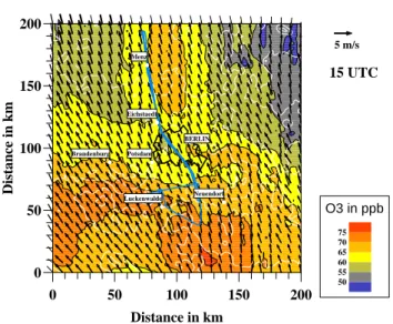
The ozone concentration distribution near ground level at 15:00 UTC on 20 July 1998, shows a pronounced ozone plume downwind of the city of Berlin (Fig. 2). The maxi-mum ozone concentration in this plume is 68 ppb. It occurs at a distance of about 70 km. Air masses with high ozone concentrations are transported over the southern boundary of the model domain.

0 50 100 150 200 Distance in km 0 50 100 150 200 Distance in km 50 55 60 65 70 75 O3 in ppb 15 UTC Brandenburg

.

.

.

.

.

.

Fig. 2. Wind and ozone concentration fields near ground level for 20 July 1998 and afternoon flight track of the IBUF aircraft.

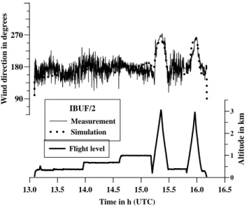
The diurnal ozone concentration cycles at two stations are presented in Fig. 3. At the Eichstaedt station, roughly 30 km downwind of the city centre of Berlin, the simulated ozone concentrations fit measurements quite well. However, at Menz station, about 70 km downwind of the city centre, the simulated ozone concentrations underestimate the mea-sured ones. A similar result is obtained when comparing the ozone concentrations measured along the flight track of the IBUF aircraft (see Fig. 2) with the corresponding simulated concentrations. The flight track begins on the upwind side about 50 km southwest of Berlin, crosses the city, and it ends

0 2 4 6 8 10 12 14 16 18 20 Time in UTC 0 10 20 30 40 50 60 70 80

Ozone concentration in ppb Measurement_{Simul. K/D - 2km}

Simul. K/D - 20km

Eichstaedt

Ozone concentration in ppb Measurement_{Simul. K/D - 2km}

Simul. K/D - 20km

Menz

Fig. 3. Diurnal cycle of ozone concentration measured at ground level for the Eichstaedt and Menz stations compared to the results simulated with 2 km and 20 km grid resolution (see Sect. 3.2).

90 180 270

Wind direction in degrees

Measurement Simulation IBUF/2 13.0 13.5 14.0 14.5 15.0 15.5 16.0 16.5 Time in h (UTC) 0 1 2 3 Altitude in km Flight level

Fig. 4. Comparison of wind direction along the flight track of IBUF.

about 100 km downwind. Along this flight track, the air-craft flew at different altitudes. As can be seen from Fig. 4, the wind direction measured during the flight is simulated well by the model. A similar agreement is found for the wind speed, the temperature and the humidity. The simu-lated ozone concentration along the flight track also agrees quite well with the observations, except for two time periods (13.8 UTC and 15.1 UTC). During these two periods the air-craft flew in the area around and north of Menz where the model underestimates the measured ozone values by about 10–15 ppb (Fig. 5), while the meteorological conditions are simulated well. 50 60 70 80 Ozone concentration in ppb Measurement Simulation IBUF/2 13.0 13.5 14.0 14.5 15.0 15.5 16.0 16.5 Time in h (UTC) 0 1 2 3 Altitude in km Flight level

Fig. 5. Comparison of ozone concentration along the flight track of IBUF.

2.3 Mass budget components of ozone in four layers over three regions

The mass budget module in the KAMM/DRAIS model cal-culates the contributions of different processes to the change in the mean concentration in a predefined volume (Fig. 6). Production and loss terms are marked P and L, respectively. More details are published in Panitz et al. (2002).

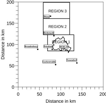
The calculations were performed for three regions (Fig. 7). The first region comprises the city of Berlin, two others are located north of the city. The ozone plume of the city crosses

Chemical Transformation Chemical Transformation LCH advective und turbulent Fluxes Temporal Change of Mass

Emission PE Deposition LD in vertical advective and turbulent Fluxes

out PCH t M ∂ ∂ advective and turbulent Fluxes PADV + PTRB LADV + LTRB

Fig. 6. Illustration of mass budget components.

these two regions during the afternoon. The atmospheric column over each region was divided into four vertical layers:

Layer 1: 2000 m–5000 m (free troposphere) Layer 2: 1200 m–2000 m (upper boundary layer) Layer 3: 75 m–1200 m (lower boundary layer) Layer 4: ground–75 m (surface layer)

These layers have been chosen with respect to the boundary layer structure during the afternoon, when the aircraft measurements took place. They have to be the same over the whole simulation period in order to allow a comparison of the results. Although all mass budget components were determined, only the changes in ozone concentration due to chemical transformations are presented. Determining this quantity was one of the purposes of the experiment. Figure 8 shows the hourly change in the chemical ozone net production rate in layer 3 above all regions. During the afternoon hours, the net production rates are nearly the same in the regions 1 and 2, whereas the rate is obviously lower in region 3.

During the afternoon the ozone net production in the ur-ban plume reaches a level of about 6.5±1.0 ppb/h, as derived from aircraft measurements on the downwind side of the city (Corsmeier et al., 2002). The aircraft flew at different levels in the lower mixing layer (layer 3 in our mass balance cal-culations), and it crossed regions 2 and 3 several times. The simulated ozone net production rate has been averaged over the time periods when the aircraft crossed the two regions, resulting in 5.1 ppb/h and 3.5 ppb/h for regions 2 and 3, re-spectively. For region 2 this is still in acceptable agreement with the value derived from the aircraft measurements. The ozone net production rate in region 3 is obviously too low. For the city region, values of 4.5±1.0 ppb/h and 5.0 ppb/h are calculated for the measured and the simulated ozone net production rates, respectively.

The results of this comparison give an indication that the reason for the underestimation of the observed ozone

con-0 50 100 150 200 Distance in km 0 50 100 150 200 Distance in km REGION 1 REGION 2 REGION 3 Brandenburg

.

.

.

.

.

.

Fig. 7. Arrangement of regions.

Fig. 8. Diurnal cycle of ozone production rate caused by chemical reactions in layer 3 over three regions.

centrations at Menz by the model might be caused by too low ozone net production rate in the city plume at farther distances.

3 Sensitivity analysis

A sensitivity study was performed to find the reasons of the discrepancies identified in ozone concentrations. In our case, sensitivity is defined as the parameter derivative ∂J /∂p of a distance function, J . This function is defined as

J = 2 X l=1 16 X i=8 (Cs,i−Cm,i)2l (1)

with:

Cs,i: simulated ozone concentration for the time i (UTC),

Cm,i: measured ozone concentration for the time i (UTC),

l=1: at Eichstaedt station (see Figs. 2 and 3), l=2: at Menz station (see Figs. 2 and 3).

The value of the distance function describes the qual-ity of the agreement between the measured and the calculated ozone concentrations at the stations Eichstaedt and Menz during daytime. The lower the value is, the better the agreement. The ozone concentrations at both stations were selected as representative for the ozone concentrations in the plume closer and farther away from the city of Berlin.

Four parameters are selected for the analysis: – Emissions,

– initial species concentrations,

– boundary values of species concentrations, – reaction rates

Meteorological variables are not considered as model para-meters, because, on one hand, we put much effort into the modelling of the meteorological conditions. In order to get a good agreement between measured and simulated meteoro-logical quantities, several simulations with the meteorologi-cal model KAMM have been carried out using the nudging procedure being part of the model system. Wind speed and direction as well as temperature and humidity along the flight route of the IBUF aircraft are well simulated. The bound-ary layer height derived from the aircraft measurements may vary between 1500 m and 1800 m compared to the modelled value of about 1600 m.

On the other hand, from the model’s underestimation of the net ozone production rate in the city plume at farther dis-tances it can be assumed, that parameters of the chemistry model are probably responsible for the ozone deficits found at Menz station.

Furthermore, the BERLIOZ episode we are considering has also been modelled with the EURAD model. This model uses the same chemical mechanism as the DRAIS model does. But the parameterizations in the meteorological part are different from those in the KAMM model. However, the results of both model systems show similar ozone concentra-tions at the station Menz. This is an additional indication that the deficit, we are looking for, is not caused by the meteoro-logical model.

Several possibilities exist to calculate the sensitivities de-scribed before. Since we are interested in the sensitivities of the distance function related to a large number of parame-ters at all grid points of the model domain, it is necessary to have a methodology that allows calculating these sensitivities simultaneously. Such an effective way of calculating the sen-sitivities is the application of an adjoint model. Although the

development of such a model is not easy and a long lasting task, it has been carried out resulting in the adjoint DRAIS model.

3.1 The adjoint DRAIS model

The sensitivities described before can be calculated with the tangent linear model, which is determined by building the derivative of the variables of the original model related to a model parameter, ∂C/∂p. Because the sensitivities of the distance function depend on these variables, they can be cal-culated using the results of the tangent linear model. The dis-advantage of this method is the fact that for each parameter a separate simulation has to be carried out. It would be much more effective if the sensitivities of the distance function re-lated to many parameters can be calcure-lated simultaneously. Using the adjoint model instead of the tangent linear model allows such an effective calculation. The adjoint model can be derived from the tangent linear model by applying the re-lation between both model operators and variables, which is given by Eq. (2).

< g∗;M0g >=< M0∗g∗;g > (2) where

<A;B> is the symbol of the inner product of the expressions

Aand B.

g= gradient, (∂C/∂p), which is the variable in the tangent linear DRAIS model

g∗= adjoint gradient, which is the variable in the adjoint DRAIS model

M0= model operator of the tangent linear DRAIS model M0∗= model operator of the adjoint DRAIS model.

The derivation of the adjoint model equations is not the task of this paper. There are several publications (Talagrand and Courtier, 1987; Pudykiewicz, 1998; Ustinov, 2001), where the procedures are presented in more detail.

Although programmes exist for automatic transformation of the original code into the tangent linear and the adjoint codes (TAMC, Giering and Kaminski, 1998; Odyssee, Ros-taing et al., 1993), the adjoint DRAIS model was developed manually. Unlike the adjoint CHIMERE model (Schmidt and Martin, 2003), however, it is not coded line by line in accordance with the principles of automatic transformation. The adjoint DRAIS model is derived from the tangent linear model of DRAIS, which uses the same difference approx-imations as the original model. Equation (2) is applied to determine the adjoint DRAIS model equations as in the pro-cedure given by Ustinov (2001). Instead of differential equa-tions, difference equations are used to obtain the adjoint dif-ference equations. This is advantageous because the results of the sensitivity analysis using the adjoint model can be bet-ter compared with those achieved when applying the tangent linear and the original models. The structure of the adjoint DRAIS model is similar to that of the original model and

the tangent linear model. Of course, the subprograms are ar-ranged in inverse order. As far as possible the subprograms are coded corresponding to the original model. These man-ually coded programmes offer the advantage of clear struc-tures and can be optimized with respect to storage require-ments and computing time (Elizondo et al., 2002).

3.1.1 Advection scheme

In the original DRAIS model, a second-order non-oscillatory Flux Corrected Transport (FCT) advection scheme with lim-iters is implemented. In addition, divergence correction is used. To avoid problems in the adjoint scheme (Thuburn and Haine, 2001), this scheme was used without limiters. It is now linear and of second order, but no longer monotone. The results of the original and the modified advection schemes differ only slightly. The distance function (Eq. 1) decreases by only approx. 3%. The adjoint advection term was derived from Eq. (2) with the modified difference scheme used for advection. It differs slightly from the tangent linear advec-tion scheme with inverse velocities. The divergence correc-tion term is omitted in the adjoint adveccorrec-tion scheme.

3.1.2 Diffusion scheme

Diffusion is approximated in the original and the tangent lin-ear model by central differences. This approximation can also be applied in the adjoint DRAIS model using the adjoint deposition velocity.

3.1.3 Chemical reaction terms

The chemical reaction terms in the original DRAIS model are non linear. They are linearized in the tangent linear model. The linearized chemical reaction terms can be written as an n×n matrix, where n is the number of variables, ∂ Ck/∂ p, in

the tangent linear model.

d(∂ Ck/∂ p)/dt = n

X

i=1

Ak,i∂ Ck,i/∂p k =1, n (3)

These variables are the model parameter derivatives of the chemical species concentrations in the original DRAIS model. In the DRAIS model, 41 transported and 18 di-agnosed species are considered, thus, n=59. In the adjoint DRAIS model, the transpose of this matrix is employed. The procedure to solve Eq. (3) is the same in both models and cor-responds to the QSSA method used to integrate the RADM2 chemical mechanism (Chang et al., 1987).

3.1.4 Test calculations

The correctness of the adjoint DRAIS model was tested by sensitivity calculations for a large number of model parame-ters at different grid points. The sensitivities of the distance function calculated by applying the adjoint DRAIS model are compared with the sensitivities derived from two simulations

with the original model using the parameter values, p±1p. The comparisons have been performed not only at those grid points with the highest sensitivity values, but also at a lot of other grid points. Of course, the results were not identical. After the test calculations the relative error between both re-sults was less than 1%, at least for the higher sensitivity val-ues.

3.2 Results of sensitivity analysis

The sensitivity of the distance function relative to the para-meters mentioned above is calculated for each grid point. For these calculations, the grid size was increased by a factor of 10 because of the large number of data to be stored. In ad-dition, the simplified data assimilation (Sect. 4) takes a lot of computing time. The increase in grid size allows a large number of simulations to be run with acceptable storage and run times. Also, more test calculations can be performed. The KAMM/DRAIS simulations (Sect. 2.2) were repeated with a coarse horizontal resolution of 20 km. During the day, differences between the diurnal cycles of ozone concentra-tions resulting from simulaconcentra-tions with grid resoluconcentra-tions of 2 km and 20 km are rather small at both stations, Eichstaedt and Menz (Fig. 3). Therefore, it may be sufficient to calculate sensitivities with the coarser grid.

The sensitivity, Sp, of the distance function, J , relative to

a model parameter p is defined as:

Sp=∂J /∂p (4)

In the analysis below, the parameter, p, is replaced by the reference value, po, multiplied by a factor, fp, which is the

new parameter replacing p. p = p0×fp

po is constant representing the original value applied in the

reference DRAIS model simulation. This transformation is helpful for those parameters, which are time dependent like the emissions. By using fp instead of p, the sensitivity

de-pends only on the level and not on the shape of the diurnal variation of parameter p. For a better comparison of the sen-sitivities this transformation was applied to all parameters.

The sensitivity (Eq. 4) is now defined as: Sp=(∂J /∂fp)/p0=Sfp/p0

with

Sfp=∂J /∂fp. (5)

The sensitivity, Sfp, used below, is now related to the

param-eter, fp.

The simulation starts at 00:00 UTC and runs till 05:00 UTC. The results of this first run are used as initial conditions for a second one running from 05:00 UTC till 21:00 UTC. The time of initialization for the calculation of the sensitivities is 05:00 UTC. This initialization time was

0 5 10 15 20 Species emitted -50 0 50 100 150 200

Max. sensitivity of the distance function in ppb

2 SO2 SULF NO2 NO ALD HCHO ORA2 NH3 HC3 HC5 HC8 ETH CO OL2 OLT OLI TOL XYL KET CSL ISO

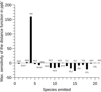
Fig. 9. Maximum sensitivity of the distance function related to the emissions.

chosen, because it is short after sunrise, when daytime chem-istry is activated. Additionally, the ozone concentration cal-culated at the station Menz is still close to the measured value. Deviations occur only later during the day.

3.2.1 Emissions

The sensitivity of the distance function related to emissions,

Sf e=∂J /∂fe (6)

is calculated for all grid points where emissions occur, and for all species emitted. The local maximum of Sf efor each

species, integrated over the time between 05:00 UTC and 16:00 UTC, is plotted in Fig. 9 arranged by the numbers they posses in the emission inventory of the original DRAIS model (see Appendix A). Negative sensitivity means that an increase in emissions of this species reduces the distance function, thus furnishing better agreement of the measured and the simulated ozone concentrations at the stations Eich-staedt and Menz. As the distance function, J , depends on the ozone concentrations, it is no surprise that NO is the most sensitive species. High values of positive sensitivity related to NO emissions occur in the area of the city of Berlin close to the ground and also in higher levels. Negative sensitivities occur also close to the ground but upwind of the city. But the highest absolute value occurring in these regions is more than a factor 10 lower than the maximum sensitivity of about 160 ppb2that is found in the city of Berlin.

The main sensitivities related to the hydrocarbons appear close to the ground in and around the city of Berlin. Only negative sensitivities are calculated. The maximum values of the sensitivities relative to hydrocarbons are located at the

same grid point in the centre of the model domain. If the peak values are summed up, the absolute value is about 10% lower than the maximum sensitivity relative to NO. This means that the influence of the hydrocarbon emissions on the distance function is nearly the same as the influence of the NO emis-sions, but with inverse sign. The peak sensitivity related to alkenes emissions is higher than those of alkanes, carbonyls, and aldehydes. The sensitivity related to CO emissions cor-responds to that of aldehydes. To obtain a lower distance function, NO emissions must be reduced while hydrocarbon and CO emissions must be increased. Beside the local maxi-mum sensitivities those integrated over the whole domain are calculated. Based on absolute values, the sensitivity ranking does not change. It is the same as for the consideration of local maxima. But the sensitivity relative to NO emissions is nearly a factor of two higher than the absolute value of the sensitivity related to the hydrocarbon emissions.

3.2.2 Initial species concentrations

The sensitivity of the distance function relative to initial species concentrations is defined as in the previous case:

Sf i=∂J /∂fi (7)

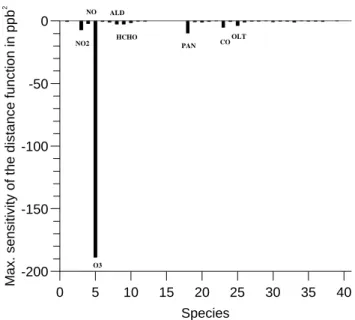
The sensitivities are calculated at each grid point for all 41 species listed in Appendix A. Again, the local maximum sensitivity for each species integrated over the time between 05:00 UTC and 16:00 UTC is considered (Fig. 10). As the distance function depends on the ozone concentration, ozone is expected to be the most sensitive species. The local peak sensitivity for ozone (−123 ppb2) is really the dominant sen-sitivity. The peak value occurs west of the city centre in a height of about 750 m above ground. Further considerable values are found upwind of the city, also at higher levels. The second species in the ranking list is PAN. Its peak sensi-tivity value is about a factor of 20 lower than that for ozone. Thus, it can be concluded that modifications of the concen-trations of all non ozone species have only a minor influence on the distance function. This statement is confirmed by the sensitivities integrated over the model domain. A special role plays the sensitivity with respect to NOxwhose peak value

is positive in contrast to the sensitivities for all other species. Considerable positive sensitivities related to NOxare found

in and around Berlin up to a height of 500 m. In still higher levels the sensitivities are negative. Close to the ground the sensitivities related to the initial NOx concentrations show

the same positive sign as for the NOxemissions. But in the

upper levels there is another regime, where an increase of the NOxconcentration causes a production of ozone downwind

of the city. Because of these two different regimes, the sen-sitivity for NOx integrated over the model domain does not

reflect the real importance of this species compared to the other non ozone species. Therefore, its place in the ranking (absolute values) of the integrated sensitivities is below that of the ranking list based on the local peak sensitivities.

0 5 10 15 20 25 30 35 40 Species -150 -100 -50 0

Max. sensitivity of the distance function in ppb

2 NO2 NO O3 HCHO PAN CO OLT

Fig. 10. Maximum sensitivity of the distance function related to the initial conditions.

3.2.3 Boundary species concentrations

The sensitivity with respect to the boundary species concen-trations is defined in the same way as for the previous para-meters.

Sf b=∂J /∂fb (8)

Boundary values are taken into account for those 41 species listed in Appendix A. Figure 11 shows the maximum sen-sitivity related to all these species. As expected, the most sensitive species again is ozone. Two maxima occur at the western and southern boundary. The negative peak value (−189 ppb2) is located in a height of 1900 m above ground at the western boundary, about 80 km north of the south-west corner of the model domain. An absolute sensitivity max-imum in such an altitude at the western boundary is only found for ozone. It can only be explained by the fact that ozone is transported to the area of Menz in the upper lay-ers, and then mixed down to the ground. The secondary peak value for ozone (−98 ppb2) is located 60 km east of the south-west corner in a height of 1100 m. Between these two peaks, further sensitivities with rather high values occur along the western and southern boundary. Corresponding to the results for the initial conditions, the maximum sensitivity for PAN is about a factor of 20 lower than that for ozone. It is located at the southern boundary, 80 km east of the south-west corner in a height of about 700 m above ground. The maximum sensitivity related to the hydrocarbons is lower than that for the initial hydrocarbons. The peak sensitivity values are also located at the southern boundary in altitudes between 100 and 700 m. Different to the result for the initial conditions is the sensitivity for NOx. No positive sensitivities

0 5 10 15 20 25 30 35 40 Species -200 -150 -100 -50 0

Max. sensitivity of the distance function in ppb

2 O3 NO2 NO CO HCHO ALD OLT PAN

Fig. 11. Maximum sensitivity of the distance function related to the boundary conditions.

are calculated and the shape of the distribution of the sensitiv-ities at the southern boundary is similar to that of PAN. At the southern boundary there is a low NOxconcentration regime

resulting in negative sensitivity values for NOx. If we look

to the sensitivities for the different species concentrations in-tegrated over the model domain, the ranking of the absolute values is similar to that for the local peak sensitivities. This means that the integrated sensitivities provide no important further information. The sensitivity values for all species are negative. Therefore, a decrease of the distance function re-quires an increase of the concentrations at the western and southern boundary.

3.2.4 Photolysis rates

The sensitivities of the distance function with respect to the photolysis rates,

Sfp=∂J /∂fp (9)

are calculated at all grid points and for all 21 photolysis reac-tions (Stockwell, 1990). The local maximum values for each photolysis rate integrated over the time between 05:00 UTC and 16:00 UTC are plotted in Fig. 12. Reaction (1) describes the photolysis of NO2to NO and O3(see Table 1). This is

the most important photolysis reaction influencing the pro-duction of ozone. Therefore, it is not astonishing that the peak sensitivity for this reaction rate is the dominant one in Fig. 12. The local maximum sensitivity (−172 ppb2)is lo-cated close to the ground in the area of Menz. Further high sensitivity values are found up to a height of 750 m. Lower sensitivities are calculated at grid points south of the Menz area in the same layer, The next important reaction is the

2100 K. Nester and H.-J. Panitz: Sensitivity analysis for BERLIOZ

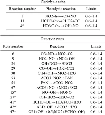
Table 1. Parameters modified in simplified data assimilation together with the lower and upper limits of fp(*reactions additionally considered

in the assimilation process).

18 K. Nester and H.-J. Panitz: Sensitivity analysis for BERLIOZ

Table 11. Parameters modified in simplified data assimilation together with the lower and upper limits of fp(*reactions additionally

consid-ered in the assimilation process).

Emissions

Classes Species group Species name Limit

1 SO2 Sulfur dioxide 0.66–1.5

2 NO2 Nitrogen dioxide 0.66–1.5

3 NO Nitric oxide 0.66–1.5 4 ALD+HCHO+KET Carbonyls 0.5–2.0 5 HC3+HC5+HC8+ETH Alkanes 0.5–2.0 6 CO Carbon monoxide 0.5–2.0 7 OL2+OLT+OLI+ISO Alkenes 0.5–2.0 8 TOL+XYL+CSL Aromatics 0.5–2.0

Initial concentrations and boundary concentrations

Species number Species Limits of Limits of

in the model init. conc. bound. conc.

3 NO2 0.75–1.3 0.6–1.4 4 NO 0.66–1.5 0.6–1.4 5 O3 0.83–1.2 0.6–1.4 9 HCHO 0.66–1.5 0.6–1.4 18 PAN 0.66–1.5 0.6–1.4 23 CO 0.66–1.5 0.6–1.4 25 OLT 0.66–1.5 0.6–1.4 Photolysis rates

Reaction number Photolysis reaction Limits

1 NO2+hv→O3+NO 0.6–1.4

11 HCHO+hv→2HO2+CO 0.6–1.4

4* HONO+hv→OH+NO 0.6–1.4

Reaction rates

Rate number Reaction Limits

6 O3+NO→NO2+O2 0.6–1.4 9 HO2+NO→NO2+OH 0.6–1.4 24 OH+NO2→HNO3 0.6–1.4 29 CO+OH→HO2+CO2 0.6–1.4 30 CH4+OH→MO2+H2O 0.6–1.4 53 ACO3+NO2→PAN 0.6–1.4 54 PAN→ACO3+NO2 0.6–1.4 67 ACO3+NO→MO2+NO2 0.6–1.4 15* NO+OH→HONO 0.6–1.4 27* OH+HO2→H2O+O2 0.6–1.4 41* HCHO+OH→HO2+CO+H2O 0.6–1.4 42* ALD+OH→ACO3+H2O 0.6–1.4 47* OP1+OH→0.5(MO2+HCHO+OH) 0.6–1.4

Atmos. Chem. Phys., 6, 1–18, 2006 www.atmos-chem-phys.net/6/1/2006/

Table 11. Parameters modified in simplified data assimilation together with the lower and upper limits of fp(*reactions additionally

consid-ered in the assimilation process).

Emissions

Classes Species group Species name Limit 1 SO2 Sulfur dioxide 0.66–1.5 2 NO2 Nitrogen dioxide 0.66–1.5 3 NO Nitric oxide 0.66–1.5 4 ALD+HCHO+KET Carbonyls 0.5–2.0 5 HC3+HC5+HC8+ETH Alkanes 0.5–2.0 6 CO Carbon monoxide 0.5–2.0 7 OL2+OLT+OLI+ISO Alkenes 0.5–2.0 8 TOL+XYL+CSL Aromatics 0.5–2.0

Initial concentrations and boundary concentrations Species number Species Limits of Limits of

in the model init. conc. bound. conc. 3 NO2 0.75–1.3 0.6–1.4 4 NO 0.66–1.5 0.6–1.4 5 O3 0.83–1.2 0.6–1.4 9 HCHO 0.66–1.5 0.6–1.4 18 PAN 0.66–1.5 0.6–1.4 23 CO 0.66–1.5 0.6–1.4 25 OLT 0.66–1.5 0.6–1.4 Photolysis rates

Reaction number Photolysis reaction Limits 1 NO2+hv→O3+NO 0.6–1.4 11 HCHO+hv→2HO2+CO 0.6–1.4 4* HONO+hv→OH+NO 0.6–1.4

Reaction rates

Rate number Reaction Limits 6 O3+NO→NO2+O2 0.6–1.4 9 HO2+NO→NO2+OH 0.6–1.4 24 OH+NO2→HNO3 0.6–1.4 29 CO+OH→HO2+CO2 0.6–1.4 30 CH4+OH→MO2+H2O 0.6–1.4 53 ACO3+NO2→PAN 0.6–1.4 54 PAN→ACO3+NO2 0.6–1.4 67 ACO3+NO→MO2+NO2 0.6–1.4 15* NO+OH→HONO 0.6–1.4 27* OH+HO2→H2O+O2 0.6–1.4 41* HCHO+OH→HO2+CO+H2O 0.6–1.4 42* ALD+OH→ACO3+H2O 0.6–1.4 47* OP1+OH→0.5(MO2+HCHO+OH) 0.6–1.4

Atmos. Chem. Phys., 6, 1–18, 2006 www.atmos-chem-phys.net/6/1/2006/

0 5 10 15 20

Number of photolysis reaction -200

-150 -100 -50 0

Max. sensitivity of the distance function in ppb

2

Fig. 12. Maximum sensitivity of the distance function related to the photolysis rates.

photolysis of formaldehyde (CH2O) to HO2and CO

(Reac-tion 11, Table 1), The peak sensitivity related to this photol-ysis rate occurs in the area of Menz in an altitude of 400 m

above ground. Further high sensitivities are calculated be-tween the ground and 750 m in the area of Menz and south of it. The third place in the ranking of maximum sensitivi-ties belongs to reaction number 10, the photolysis of HCHO to H2and CO. It is the largest positive maximum sensitivity.

However, this peak sensitivity is already a factor of 10 lower than that for the photolysis rate number 11. The sensitivi-ties for the photolysis rates integrated over the model domain show the same ranking (Reaction 1, followed by 11 and 10). Only the ratios between the absolute values of the three in-tegrated sensitivities are reduced by about 35% compared to the corresponding ratios of the local peak sensitivities.

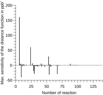
3.2.5 Reaction rates

140 non photolytic reactions are considered in the RADM2 chemical mechanism. The sensitivities of the distance func-tion related to these reacfunc-tions rates

Sf r =∂J /∂fr (10)

integrated over the time between 05:00 UTC and 16:00 UTC are calculated at each grid point. The resulting local maxi-mum sensitivities are plotted in Fig. 13. The eight dominant reactions are listed in Table 1 (the first eight reactions). As expected, the rate of the reaction between O3and NO shows

the area of Menz close to the ground. High values are also found up to an altitude of about 1500 m. In this layer remark-able sensitivity values are also located south of the Menz area. As can be seen from Table 1, the dominant sensitiv-ities are related to reactions with NO, NO2, PAN, and OH.

Out of the eight peak sensitivities, three have a positive sign (rate numbers 6, 24, and 53). They lead to a loss of ozone or NO2. The other reactions produce NO2or other species

being relevant in ozone production. The distributions of the sensitivities in the model domain related to the eight reac-tions show a shape similar to that belonging to the reaction between O3and NO.

The most relevant eight reactions based on the sensitivities integrated over the model domain and also their signs are the same as those derived from the local peak sensitivity values. Most of these reactions are also considered in the sensitivity study by Menut (2003).

4 Variation of relevant parameters

After calculation of the sensitivities it is possible to select the most relevant parameters that influence the distance function. The selection can be based on the peak sensitivities or on the sensitivities integrated over the model domain. In most cases both data bases provide the same result. But in those cases where the sensitivity distribution shows larger negative and larger positive values, the ranking of the integrated sen-sitivities does not represent the real importance of the corre-sponding parameter. Therefore, a ranking of the parameter relevance based on the absolute values of the local peak sen-sitivities is more reliable. The parameters selected are sum-marized in Table 1.

From the data in Table 1 it cannot be decided, which pa-rameter is most likely responsible for the observed discrep-ancies in the ozone concentrations at the station Menz. In order to answer this question, we carried out simplified 4-D data assimilation. It was conducted to find out which pa-rameter modifications are able to diminish discrepancies in ozone concentrations in the city plume of Berlin observed at greater distances. In this context simplified means that a background term in the distance function is not considered. This simplified data assimilation provides a lower distance function compared to one which takes a background term into account.

The main reason for using simplified data assimilation is the lower expenditure and the not (well) known error corre-lation matrix in the background term. The modified distribu-tion of the relevant parameters in the model domain is less smooth than that calculated by data assimilation with back-ground term. Because the main variations should be similar, the answer of the question risen before can be found also with the results of the simplified data assimilation. In order to avoid completely unrealistic results, parameter variation is

0 25 50 75 100 125 Number of reaction -50 0 50 100 150 200

Max. sensitivity of the distance function in ppb

2

Fig. 13. Maximum sensitivity of the distance function related to the reaction rates.

limited. The limits for the different parameters are also listed in Table 1.

The limits for emissions are estimated from evaluations of the Augsburg project (Slemr et al., 2002). For SO2, NO and

NO2 emissions, the same uncertainty factor of 1.5 is used.

Thus, the lower limit of fpis 1/1.5=0.66 and the upper limit

is 1.5. Hydrocarbon and CO emissions are more uncertain. Therefore, a value of 2.0 is chosen, which corresponds to a lower limit of 0.5.

The limits for the initial concentrations are estimated in a similar way. For the initial NO concentration, the same limits are used as for the NO emissions, because the NO concentra-tions mainly depend on local emissions. Nester and Panitz (2004) showed that differences of 20% can occur between the measured and the simulated ozone concentrations. There-fore, an uncertainty factor of 1.2 is taken for ozone. The uncertainty in the initial NO2concentration lies between the

values for NO and those for ozone because it is influenced more by chemical processes and long range transport than the NO concentration. The uncertainty factor for the initial hydrocarbon concentrations should be lower than that of the emissions. Therefore, a value of 1.5 is chosen. This value is taken also for the initial concentrations of PAN and CO.

As it is very difficult to define individual limits for the dif-ferent parameters, the same limitations were chosen for the boundary conditions and the reaction rates. For both param-eter sets, a variation of ±40% is allowed (Menut, 2003). In order to avoid unrealistic parameter modifications, this rough estimate of the limits seems to be acceptable.

All simulations with the modified parameters started at 05:00 UTC and ran till 21:00 UTC in the evening. 05:00 UTC was chosen as initialization time, because it is

0 5 10 15 20 25 30 Iteration steps 0 500 1000 1500 2000 2500 3000

Value of the distance function in ppb

2

Emi+ini.cond. with limits Reaction rates with limits Bound.cond. with limits

Fig. 14. Iterative reduction of the distance function.

short after sunrise, when daytime chemistry is activated. Ad-ditionally, the ozone concentration calculated at the station Menz is still close to the measured value. The assimilation window began at 08:00 UTC and ended at 16:00 UTC. Only in this time period, improved agreement between the mea-sured and the simulated ozone concentrations at the stations of Eichstaedt and Menz is assured. It is interesting to see whether there is better agreement also between 05:00 UTC and 08:00 UTC as well as after 16:00 UTC.

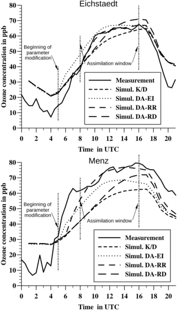
Simplified data assimilation is carried out separately with i) the initial conditions together with the emissions, as rec-ommended by Elbern and Schmidt (2002), ii) the boundary conditions, and iii) the reaction rates including photolysis rates., respectively. Iterative reduction of the distance func-tion is performed by the conjugate gradient method using limits. The convergence of the distance function is plotted in Fig. 14.

The boundary conditions furnish the highest minimum of the distance function. This result is not surprising, because it takes more than 3 h that modifications in the boundary con-ditions cause modifications in ozone concentrations at the two stations considered in the distance function. Moreover, ozone concentrations are modified similarly at both stations. At Menz agreement cannot be improved significantly with-out overestimating the ozone concentrations at Eichstaedt. This effect is reflected in the modified diurnal cycles of the ozone concentration for both stations drawn in Fig. 15.

The lowest minimum of the distance function is calculated for the reaction rates. Ozone concentrations at the Menz and Eichstaedt stations based on the modified reaction rates agree quite well with the observations in the assimilation window (Fig. 15). This indicates that uncertainties in the reaction rates may be the cause of the discrepancies in ozone con-centration. The sensitivity analysis of the photolysis rates shows that in the area of Menz and south of it high

nega-0 2 4 6 8 10 12 14 16 18 20 Time in UTC 0 10 20 30 40 50 60 70 80 Ozone concentration in ppb Measurement Simul. K/D Simul. DA-EI Simul. DA-RR Simul. DA-RD Assimilation window Beginning of modification parameter

Eichstaedt

Menz

Fig. 15. Diurnal cycle of the ozone concentration at ground level for the stations of Eichstaedt and Menz (K/D: Reference case with 20 km resolution, DA: Data assimilation, EI: Emissions and Initial concentrations; RR: Photolysis – and other Reaction Rates; RD: Boundary concentrations).

tive sensitivity values are calculated up to a height of about 750 m. After the data assimilation, the NO2photolysis rate

in this volume is increased by the limiting factor of 1.4. Be-cause the NO2photolysis rates used in the basic simulation

are valid for standard conditions without clouds, such a great increase is not probable over the whole day. Similar results are found for the modified CH2O photolysis rate and other

relevant reaction rates. This means that the good agreement of the ozone concentrations at the Eichstaedt and Menz sta-tions are probably caused by unrealistic modificasta-tions of the photolysis and reaction rates.

Varying the emissions together with the initial conditions furnishes less satisfactory agreement than modifying the re-action rates does. In the volume around and above Berlin, which is the most sensitive region, the emissions can reach also their maximum possible modifications after the simpli-fied data assimilation. Although these modifications may be more realistic than in the previous case, the observed dis-crepancies in the ozone concentration can only be partly ex-plained. It seems that errors in only one type of parameter cannot explain the ozone discrepancies at Menz station.

In the late afternoon, after 16:00 UTC (the end of assimi-lation), the ozone concentrations in the KAMM/DRAIS ref-erence simulation and in all runs with modified parameters converge relatively fast. Especially, the increased ozone con-centration at the station Menz after 16:00 UTC is simulated properly neither by the reference run nor by the runs with modified model parameters. This is an indication that addi-tional reasons could still be responsible for the discrepancies between the measured and the calculated ozone concentra-tions at Menz station. In order to check the results discussed above, corresponding comparisons have been carried out based on the ozone concentrations at the stations Lotharhof and Neuglobsow, which are located 15 km west-south-west of Menz and 12 km north-north-west of Eichst¨adt, respec-tively. The results for the station Lotharhof confirm those for the station Menz. For Neuglobsow the results are similar to those for the station Eichst¨adt. But the best agreement is not found for the modified reaction rates. This is an additional indication that the modified reaction rates may not be realis-tic.

5 Conclusions

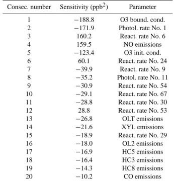
On 20 July 1998, a day in the BERLIOZ experiment, an ozone plume developed downwind of the city of Berlin. Al-though the meteorological conditions and ozone concentra-tions on the upwind side of the city are well simulated by the model, the maximum increase in ozone concentration as observed in the plume is underestimated by 10–15 ppb at dis-tances of 60–80 km downwind from the city. In this area, the ozone net production rate calculated by the model is lower than that derived from aircraft measurements. A sensitivity analysis was carried out to find the reason for this underes-timation. It is based on a distance function defined as the sum of the least squares between the measured and the sim-ulated ozone concentrations at the stations of Eichstaedt and Menz during the period from 08:00 UTC until 16:00 UTC. The emissions, initial conditions and boundary conditions, and the reaction rates are taken as model parameters. The highest sensitivities are listed in Table 2 arranged by abso-lute values.

Only five parameters show a sensitivity of more than ±100 ppb2. The others are a factor of two or more lower. The first five parameters are directly related to the concentration

Table 2. Ranking of sensitivities.

Consec. number Sensitivity (ppb2) Parameter 1 −188.8 O3 bound. cond. 2 −171.9 Photol. rate No. 1 3 160.2 React. rate No. 6 4 159.5 NO emissions 5 −123.4 O3 init. cond. 6 60.1 React. rate No. 24 7 −39.9 React. rate No. 9 8 −35.2 Photol. rate No. 11 9 −30.9 React. rate No. 54 10 −29.1 React. rate No. 67 11 −28.8 React. rate No. 30 12 28.8 React. rate No. 53 13 −26.8 OLT emissions 14 −21.6 XYL emissions 15 −18.9 React. rate No. 29 16 −18.0 OL2 emissions 17 −16.9 HC5 emissions 18 −16.4 HC3 emissions 19 −14.3 HC8 emissions 20 −10.2 CO emissions

or the production of ozone. It was to be expected that other parameters, such as the hydrocarbon and CO emissions, also show relevant sensitivities (Table 2). However, their place in the ranking list and their sensitivity values depend on the problem considered.

In addition, simplified 4-D data assimilations were per-formed. The simulation with the modified reaction rates shows a remarkable reduction of the distance function. But these reaction rates seem to be unrealistic for the whole sim-ulation period. Therefore, the good agreement of the mea-sured and simulated ozone concentrations at Eichstaedt and Menz stations should not be overestimated.

The simulation with the modified emissions and initial conditions also produces a remarkable better agreement be-tween the measured and the simulated ozone concentrations compared to the reference simulation. But the high ozone concentrations in the afternoon are not completely repro-duced.

The simulation with boundary conditions modified by data assimilation cannot describe the increase of the ozone con-centration in the morning hours.

From all these results it can be concluded that the week agreement between the measured and simulated ozone con-centration at Menz station cannot be explained by an error in only one parameter set of the reference run.

Strictly speaking, the results of this study are of course ap-plicable only to the DRAIS model and the specific episode. Although we could not clearly decide which parameters are responsible for the observed discrepancies, the procedure is also applicable to other models and episodes. Discrepan-cies between measured and simulated speDiscrepan-cies concentrations are often found and they are not a typical behaviour of the KAMM/DRAIS model system. In other cases the results of

such a study may give more evidence than the results of this study. The ranking of sensitivities for other chemistry trans-port models and other questions in context with ozone con-centrations may be different, but the relevant parameters are largely the same, because they mainly determine the ozone chemistry in such type of models. Therefore, it is not neces-sary to repeat the whole sensitivity calculations. They can be restricted to the relevant ones derived in this study.

Appendix A

List of RADM2 transported and emitted chemical species

Species Species name Chemical formula Symbol used Number in number in the model Emission inventory 1 Sulfur dioxide SO2 SO2 1

2 Sulfuric acid H2SO4 SULF 2 3 Nitrogen dioxide NO2 NO2 3

4 Nitric oxide NO NO 4

5 Ozone O3 O3

6 Nitric acid HNO3 HNO3 7 Hydrogen peroxide H2O2 H2O2

8 Acetaldehyde R-CHO ALD 5 9 Formaldehyde CH2O HCHO 6 10 Methyl hydrogen peroxide CH3OOH OP1

11 Other organic peroxides R-OOH OP2 12 Peroxyacetic acid CH3COOOH PAA 13 Formic acid HCOOH ORA1

14 Acetic acid CH3COOH ORA2 7

15 Ammonia NH3 NH3 8

16 Dinitrogen pentoxide N2O5 N2O5 17 Nitrogen trioxide NO3 NO3 18 Peroxyacetylnitrate CH3CO3NO2 PAN

19 C3 to C5 alkanes C3H8–C5H12 HC3 9 20 C6 to C8 alkanes C6H14–C8H18 HC5 10 21 Other alkanes >C10H22 HC8 11 22 Ethane C2H6 ETH 12 23 Carbon monoxide CO CO 13 24 Ethene C2H4 OL2 14

25 Terminal alkenes (propene) e.g. C3H6 OLT 15 26 Internal alkenes (butene) e.g. C4H8 OLI 16 27 Toluene CH3C6H5 TOL 17 28 Xylene (CH3)2C6H4 XYL 18 29 Acetyl peroxyl radical CH3–CO3 ACO3

30 other PAN CHOCH=CHCO3NO2 TPAN 31 Nitrous acid HNO2 HONO 32 Pernitric acid HNO4 HNO4

33 Ketones CH3COCH3, CH3COC2H5 KET 19 34 Glyoxal (CHO)2 GLY

35 Methylglyoxal CH3COCHO MGLY 36 Other dicarbonyls R-(CHO)2 DCB 37 Other organic nitrate R-ONO2 ONIT

38 Cresol HOC6H4-CH3 CSL 20

39 Isoprene C5H8 ISO 21

40 Hydroxy radical HO HO 41 Hydroperoxy radical HO2 HO2

Edited by: A. Hofzumahaus

References

Adrian, G. and Fiedler, F.: Simulation of unstationary wind and temperature fields over complex terrain and comparison with ob-servations, Contrib. Atmos. Phys., 64, 27–48, 1991.

Baer, M. and Nester, K.: Parametrization of trace gas dry de-position velocities for a regional mesoscale diffusion model, Ann. Geophys., 10, 912–923, 1992, mboxhttp://www.ann-geophys.net/10/912/1992/.

Becker, K. H., Donner, B., and G¨ab, S.: BERLIOZ: A field experi-ment within the German Tropospheric Research Programme, in: Proc. of EUROTRAC Symposium 98, vol. 2, edited by: Borrell, P. M. and Borrell, P., WIT-Press, Southampton, 669–672, 1999. Chang, J. S., Brost, A., Isaksen, I. S. A., Madronich, S., Middleton,

P., Stockwell, W. R., and Walceck, C. J.: A three-dimensional Eulerian acid deposition model: Physical concepts and formula-tion, J. Geophys. Res., 92, 14 618–14 700, 1987.

Corsmeier, U., Kalthoff, N., Vogel, B., Hammer, M.-U., Fiedler, F., Kottmeier, Ch., Volz-Thomas, A., Konrad, S., Glaser, K., Neininger, B., Lehning, M., Jaeschke, W., Memmesheimer, M., Rappengl¨uck, B., and Jakobi, G.: Ozone and PAN formation in-side and outin-side of the BERLIN plume-Process analysis and nu-merical process simulation, J. Atmos. Chem., 42, 289–321, 2002. Degrazia, G. A.: Anwendung von ¨Ahnlichkeitsverfahren auf die turbulente Diffusion in der konvektiven und stabilen Grenz-schicht, Dissertation, Fakult¨at f¨ur Physik der Universit¨at Karls-ruhe, Institut f¨ur Meteorologie und Klimaforschung, 1988. Dufour, A., Amodel, M., Ancellet, G., and Peuch, V. H.: Observed

and modelled “chemical weather” during ESCOMPTE, Atmos. Res., 74, 161–189, 2005.

Ebel, A., Elbern, H., Feldmann, H., Jakobs, H. J., Kessler, C., Memmesheimer, M., Oberreuter, A., and Piekorz, G.: Air pol-lution studies with the EURAD model system (3): EURAD-European air pollution dispersion model system, Mitteilungen aus dem Institut f¨ur Geophysik und Meteorologie der Universit¨at K¨oln, Heft 120, p. 172, 1997.

Elbern, H., Schmidt, H., Talagrand, O., and Ebel, A.: 4D-variational data assimilation with an adjoint air quality model for emission analysis, Environ. Modelling & Software, 15, 539–548, 2000. Elbern, H. and Schmidt, H.: Ozone episode analysis by

four-dimensional variational chemistry data assimilation, J. Geophys. Res., 106(D4), 3569–3590, 2001.

Elbern, H. and Schmidt, H.: The development of a 4d variational chemistry data assimilation scheme for initial value and emission rate estimates, in: Proceedings of the 6th GLOREAM Workshop, Aveiro, Portugal, 4–6 September, edited by: Borego, C., Built-jes, P., Miranda, A. I., Santos, P., and Carvalho, A. C., 123–132, 2002.

Elizondo, D., Cappelaere, B., and Faure, Ch.: Automatic ver-sus manual model differentiation to compute sensitivities and solve non-linear inverse problems, Computers & Geosciences, 28, 309–326, 2002.

Giering, R. and Kaminski, T.: Recipes for adjoint code construc-tion, ACM Transactions on Mathematical Software, 24(4), 437– 474, 1998.

Memmesheimer, M., Ebel, A., and Roemer, F.: Budget calcula-tions for ozone and its precursors: Seasonal and episodic

fea-tures based on model simulations, J. Atmos. Chem., 28, 283– 317, 1997.

Menut, L.: Adjoint modelling for atmospheric pollution process sensitivity at regional scale, J. Geophys. Res., 108(D17), ESQ 5 1–17, 2003.

Nester, K. and Fiedler, F.: Modeling of the diurnal variation of air pollutants in a mesoscale area, Proceedings of the 9th World Clean Air Congress, Montreal, 5, Paper-No. IU-16C.02, 1992. Nester, K., Fiedler, F. Panitz, H.-J., and Zhao, T.: Simulation of an

episode of the BERLIOZ experiment and comparison with mea-sured data, in: Proceedings 4th GLOREAM Workshop, Cottbus, Germany, 20–22 September, edited by: Schaller, E., Builtjes, P, and M¨unzenberg, A., 8–16, 2000.

Nester, K. and Panitz, H.-J.: Evaluation of the chemistry transport model system KAMM/DRAIS based on daytime ground level ozone data, Int. J. Environ. Pollut., 22(1/2), 87–107, 2004. Palacios, M., Kirchner, F., Martilli, A., Clappier, A., Martin, F., and

Rodrigues, M. E.: Summer ozone episodes in the Greater Madrid Area. Analyzing the ozone response to abatement strategies by modelling, Atmos. Environ., 36, 5323–5333, 2002.

Panitz, H.-J., Nester, K., and Fiedler, F.: Determination of mass balances of chemically reactive air pollutants over Baden-W¨urttemberg (F.R.G.) – Study for the regions around the cities of Stuttgart and Freudenstadt, in: Air Pollution V, edited by: Power, H., Tirabassi, T., Brebbia, C. A., Computational Mechanics Pub-lications, Southampton, Boston, 413–422, 1997.

Panitz, H.-J. and Nester, K.: Mass budget simulations of ozone in the city plume of Berlin for an episode of the BERLIOZ experiment, Companion CD-ROM of: Transport and Chemical Transformation in the Troposphere, edited by: Midgley, P. and Reuther, M., Proceedings of the EUROTRAC Symposium 2002, Garmisch-Partenkirchen, Germany, 11–15 March; see also http:// www-fzk.imk.uni-karlsruhe.de/fi/fzk/imk/seite 1513.php, 2002. Peleg, M., Luria, M., Sharf, G., Vanger, A., Kallos, G., Kotroni, V., Lagouvardos, K., and Varinou, M.: Observational evidence of an ozone episode over the Greater Athens Area, Atmos. Environ., 31, 3969–3983, 1997.

Plaza, J., Pujadas, M., and Artinano, B.: Formation and transport of the Madrid ozone plume, J. Air Waste Manage. Assoc., 47, 766–774, 1997.

Prevot, A. S. H., Staehlin, L., Kok, G. L., Schillawski, R. D., Neininger, B., Staffelbach, T., Neftel, A., Wernli, H., and Dom-men, J.: The Milan photooxidant plume, J. Geophys. Res., 102, 23 375–23 388, 1997.

Pudykiewicz, J. A.: Application of adjoint tracer transport equa-tions for evaluating source parameters, Atmos. Environ., 32(17), 3039–3050, 1998.

Rostaing, N., Dalmas, S., and Galligo, A.: Automatic differentia-tion in Odyss´ee, Tellus, 45A, 558–568, 1993.

Sch¨adler, G., Kalthoff, N., and Fiedler, F.: Validation of a model for heat, mass and momentum exchange over vegetated surfaces using LOTREX-10E/HIBE88 data, Contrib. Atmos. Phys., 63, 85–100, 1990.

Schmidt, H. and Martin, D.: Adjoint sensitivity of episodic ozone in the Paris area to emissions on the continental scale, J. Geophys. Res., 108(D17), ESQ 4 1–16, 2003.

Slemr, F., Baumbach, G., Blank, P., Corsmeier, U., Fiedler, F., Friedrich, R., Habram, M., Kalthoff, N., Klemp, D., K¨uhlwein, J., Mannschreck, K., M¨ollmann-Coers, M., Nester, K., Panitz,

H.-J., Rabl, P., Slemr, J., Vogt, U., and Wickert, B.: Evaluation of modelled spatially and temporally highly resolved emission inventories of photosmog precursors for the city of Augsburg: the experiment EVA and its major results, J. Atmos. Chem., 42, 207–233, 2002.

Stockwell, W. R., Middelton, P., and Chang, J. S.: The second gen-eration Regional Acid Deposition Model, chemical mechanism for regional air quality modeling, J. Geophys. Res., 95(D10), 16 343–16 367, 1990.

Thuburn, J. and Haine, T. W. N.: Adjoints of nonoscillatory advec-tion schemes, J. Comput. Phys., 171, 616–631, 2001.

Talagrand, O. and Courtier, P.: Variational assimilation of meteoro-logical observations with the adjoint vorticity equation. I: The-ory, Quart. J. Roy. Meteorol. Soc., 113, 1311–1328, 1987. Ustinov, E. A.: Adjoint sensitivity analysis of atmospheric

dynam-ics: Application to the case of multiple observables, J. Atmos. Sci., 58(21), 3340–3348, 2001.

Vautard, R., Beekmann, M., and Menut, L.: Applications of ad-joint modelling in atmospheric chemistry: sensitivity and inverse modelling, Environ. Modelling & Software, 25, 703–709, 2000. Vautard, R., Menut, L., Beekmann, M., Chazette, P., Flamant, P.

H., Gombert, D., Kley, D., Lefebvre, M. P., Marti, D., Megie, G., Perros, P., and Toupance, G.: A synthesis of air pollution over the Paris region (ESQUIF) field campaign, J. Geophys. Res.-Atmos., 108(D17, 8558, doi:10.1029/2003JD003380, 2003.

Vogel, B., Fiedler, F., and Vogel, H.: Influence of topography and biogenic volatile organic compounds emission in the state of Baden-W¨urttemberg on ozone concentrations during episodes of high air temperatures, J. Geophys. Res., 100, 22 907–22 928, 1995.

Wotawa, G., Stohl, A., and Neininger, B.: The urban plume of Vienna: Comparison between aircraft measurements and photo-chemical model results, Atmos. Environ., 32, 2479–2489, 1998.