HAL Id: hal-00302747
https://hal.archives-ouvertes.fr/hal-00302747
Submitted on 17 Jul 2006
HAL is a multi-disciplinary open access
archive for the deposit and dissemination of
sci-entific research documents, whether they are
pub-lished or not. The documents may come from
teaching and research institutions in France or
abroad, or from public or private research centers.
L’archive ouverte pluridisciplinaire HAL, est
destinée au dépôt et à la diffusion de documents
scientifiques de niveau recherche, publiés ou non,
émanant des établissements d’enseignement et de
recherche français ou étrangers, des laboratoires
publics ou privés.
NAO index and temperature records are
phase-synchronized
Milan Palus, D. Novotná
To cite this version:
Milan Palus, D. Novotná. Quasi-biennial oscillations extracted from the monthly NAO index and
tem-perature records are phase-synchronized. Nonlinear Processes in Geophysics, European Geosciences
Union (EGU), 2006, 13 (3), pp.287-296. �hal-00302747�
Nonlin. Processes Geophys., 13, 287–296, 2006 www.nonlin-processes-geophys.net/13/287/2006/ © Author(s) 2006. This work is licensed
under a Creative Commons License.
Nonlinear Processes
in Geophysics
Quasi-biennial oscillations extracted from the monthly NAO index
and temperature records are phase-synchronized
M. Paluˇs1and D. Novotn´a2
1Institute of Computer Science, Academy of Sciences of the Czech Republic, Pod vod´arenskou vˇeˇz´ı 2, 182 07 Prague 8, Czech Republic
2Institute of Atmospheric Physics, Academy of Sciences of the Czech Republic, Boˇcn´ı II/1401, 141 31 Prague 4, Czech Republic
Received: 20 January 2006 – Revised: 28 March 2006 – Accepted: 21 April 2006 – Published: 17 July 2006
Abstract. Using the extension of Monte Carlo Singular
Sys-tem Analysis (MC SSA), based on evaluating and testing the regularity of the dynamics of the SSA modes against the col-ored noise null hypothesis, we demonstrate detection of os-cillatory modes with period of about 27 months in records of monthly average near-surface air temperature from sev-eral European locations, as well as in the monthly North At-lantic Oscillation index. According to their period, the de-tected modes can be attributed to the quasi-biennial oscilla-tions (QBO). The QBO modes extracted from the temper-ature and from the NAO index underwent synchronization analysis and their phase synchronization has been confirmed with high statistical significance.
1 Introduction
The North Atlantic Oscillation (NAO) is a dominant pat-tern of atmospheric circulation variability in the extratropi-cal Northern Hemisphere, accounting for about 60% of the total sea-level pressure variance. The NAO has a strong ef-fect on European weather conditions, influencing meteoro-logical variables including temperature (Hurrell et al., 2001). The NAO-temperature relationship, however, is not straight-forward and its mechanism is not yet fully understood. Re-cent studies show that the relationship between the NAO and the winter Northern Hemisphere surface temperature (NHT) might be a function of the NAO state (Pozo-V´azques et al., 2001). There are energetic modes of coherent variability be-tween temperature and the NAO in the time domain of 2–6 years for 1857–1879 and 1978–1984, and in the domain of 6–10 years from 1961 to 1991 (Pozo-V´azques et al., 2001). Changes of the strength and character of correlations
be-Correspondence to: M. Paluˇs
(mp@cs.cas.cz)
tween the NAO and the NHT seems to be modulated by the phase of the solar activity cycle (Gimeno et al., 2003).
The long-term dynamical behaviour of the NAO phe-nomenon itself is far from being understood and is also in-vestigated in connection with studies of predictability of the NAO and the ability of climate numerical models of simulat-ing it (Eden et al., 2002; Bojariu and Gimeno, 2003). Some authors are pessimistic, claiming that the NAO index can be considered just as pink noise with very little predictability (Fernandez et al., 2003). On the other hand, G´amiz-Fortis et al. (2002) have applied the Monte Carlo Singular System Analysis (MC SSA) to the winter NAO index, i.e., yearly sampled values obtained by averaging December, January and February index values, and, using an embedding window of length n=40 years, were able to identify an oscillatory mode with a period of about 7.7 years. Paluˇs and Novotn´a (2004) have introduced the so called enhanced MC SSA, based on evaluating and testing the regularity of the dynam-ics of the SSA modes against the colored noise null hypothe-sis, in addition to the test based on variance (eigenvalues). The application of the regularity index, computed from a coarse-grained estimation of mutual information, enhances the test sensitivity and reliability in the detection of dynam-ical modes which are relatively more regular than those ob-tained by decomposition of colored noise, in particular, in the detection of irregular oscillations embedded in red noise. This enhanced MC SSA was successfully applied in the de-tection of oscillatory modes of period 7.8 years in records of monthly average near-surface air temperature from several European locations, as well as in the monthly North Atlantic Oscillation index (Paluˇs and Novotn´a, 2004).
In this paper we continue and refine the enhanced MC SSA analysis of the temperature records and the monthly North Atlantic Oscillation index by focusing on higher (than near-decadal) frequencies and demonstrate the presence of several oscillatory modes with periods in the range from 20 to 64 months. The most prominent oscillatory mode (besides the
above mentioned mode with period 7.8 years) is the mode with the average period 27 months. We identify this mode with the quasi-biennial oscillation (QBO) and extract this os-cillatory mode from both the temperature data and the NAO index. The extracted oscillatory modes (projections on the SSA/EOF basis) are further studied by the means of synchro-nization analysis (Pikovsky et al., 2001) and the existence of phase synchronization between the QBO modes from the temperature and from the NAO index is demonstrated and statistically proven.
A brief introduction into Monte Carlo singular system analysis and its enhancement is given in Sect. 2. The ana-lyzed data are described in Sect. 3. Section 4 summarizes the application of enhanced MC SSA to monthly average near-surface temperature records and to the monthly NAO index. Synchronization analysis is introduced and applied to the QBO modes in Sect. 5. The results are discussed in Sect. 6 and conclusions are given in Sect. 7.
2 Monte Carlo singular system analysis
Singular system (or singular spectrum) analysis (SSA) in its original form (also known as principal component analysis, or Karhunen-Lo`eve decomposition) is a method for the iden-tification and distinction from noise of important informa-tion in multivariate data. It is based on an orthogonal de-composition of a covariance matrix of multivariate data un-der study. SSA provides an orthogonal basis onto which the data can be transformed, thus making individual data compo-nents (“modes”) linearly independent. Each of the orthogo-nal modes (projections of the origiorthogo-nal data onto new orthog-onal basis vectors) is characterized by its variance, which is given by the related eigenvalue of the covariance matrix.
Here we will deal with a univariate version of SSA in which the analyzed data is a univariate time series and the decomposed matrix is a time-lag covariance matrix, i.e., in-stead of several components of multivariate data, a time se-ries and its time-lagged versions are considered. This form of SSA, which has frequently been used in the field of mete-orology and climatology (Vautard and Ghil, 1989; Ghil and Vautard, 1991; Keppenne and Ghil, 1992; Yiou et al., 1994; Allen and Smith, 1994), can provide a decomposition of the studied time series into orthogonal components (modes) with different dynamical properties, and thus “interesting” phe-nomena such as slow modes (trends) and regular or irregular oscillations (if present in the data) can be identified and re-trieved from the background of noise and/or other “uninter-esting” non-specified processes.
In traditional SSA, the distinction of “interesting” com-ponents (signal) from noise is based on finding a threshold (jump-down) to a “noise floor” in a sequence of eigenvalues given in a descending order. This approach might be prob-lematic if the signal-to-noise ratio is not sufficiently large, or the noise present in the data is not white but “colored”.
For such cases, statistical approaches utilizing Monte Carlo simulation techniques have been proposed (Ghil and Vautard, 1991; Vautard et al., 1992) for reliable signal/noise separa-tion. The particular case of Monte Carlo SSA (MC SSA) that considers “red” noise, usually present in geophysical data, has been introduced by Allen and Smith (1996).
Now, we present a few necessary details of the SSA method in the form of a technical recipe:
Take the analyzed time series {y(i)}, i=1, . . . , N0, and construct a map (“embedding”) into a space of n-dimensional vectors x(i) with components xk(i), given as
xk(i) = y(i + k −1), (1)
where k=1, . . . , n; and n is the embedding dimension. Construct a symmetric n×n matrix C=XTX, with
ele-ments: ckl=(1/N ) N X i=1 xk(i)xl(i), (2)
where 1/N is the proper normalization and the components xk(i), i=1, . . . , N , are supposed to have a zero mean. The symmetric matrix C can be decomposed as
C = V6VT, (3)
where the n×n matrix V={vij}gives an orthonormal basis
in the space of vectors x(i), 6=diag(σ1, σ2, . . . , σn), σi are
non-negative eigenvalues giving the variance of orthogonal modes ξk(i) = n X l=1 vlkxl(i), (4)
into which the original series can be decomposed. For more details, see, e.g., Vautard et al. (1992).
Of course, the original time series xk(i) can be recon-structed from the modes, as
xk(i) =
n
X
l=1
vklξl(i). (5)
In Eq. (5), the modes ξk(i)can also be interpreted as time-dependent coefficients and the orthogonal vectors vk={vkl}
as basis functions, usually called the empirical orthogonal functions (EOFs).
The clear signal/noise distinction based on the eigenvalues σ1, σ2, . . . , σncan only be obtained in particularly idealized
situation when the signal/noise ratio is large enough and the background consists of white noise. In many geophysical processes, however, so-called “red” noise with power spec-trum of the 1/f type is present (Allen and Smith, 1996). Its SSA eigenspectrum also has the 1/f character (Gao et al., 2003), i.e., an eigenspectrum of red noise is equivalent to a coarsely discretized power spectrum, where the number of frequency bins is given by the embedding dimension n. The eigenvalues related to the slow modes are much larger than
M. Paluˇs and D. Novotn´a: Phase-synchronized QBO in the NAO and temperature records 289 the eigenvalues of the modes related to higher frequencies.
Thus, in the classical SSA approach applied to red noise, the eigenvalues of the slow modes might incorrectly be in-terpreted as a (nontrivial) signal, or, on the other hand, a nontrivial signal embedded in red noise might be neglected if its variance is smaller than the slow-mode eigenvalues of the background red noise. Therefore, Allen and Smith (1996) proposed comparing the SSA spectrum of the analyzed sig-nal with SSA spectra of a red-noise model fitted to the stud-ied data. Such a red-noise process can be modeled by using an AR(1) model (autoregressive model of the first order): u(i) − ˆu = α(u(i −1) − ˆu) + γ z(i), (6) where ˆuis the process mean, α and γ are process parameters, and z(i) is Gaussian white noise with a zero mean and a unit variance.
In order to correctly detect a signal in red noise, the follow-ing approach has been proposed (Allen and Smith, 1996): First, the eigenvalues are plotted not according to their val-ues, but according to a frequency associated with a particular mode (EOF), i.e., the eigenspectrum in this form becomes a sort of a (coarsely) discretized power spectrum in general, not only in the case of red noise (when the eigenspectrum naturally has this form, as mentioned above).
Second, an eigenspectrum obtained from studied data is com-pared, in a frequency-by-frequency way, with eigenspectra obtained from a set of realizations of an appropriate noise model (such as the AR(1) model (6)), i.e., an eigenvalue re-lated to a particular frequency bin obtained from the data is compared with a range of eigenvalues related to the same frequency bin, obtained from the set of realizations of the chosen AR(1) model.
The detection of a nontrivial signal in an experimental time series becomes a statistical test in which the null hypothe-sis that the experimental data were generated by a chosen noise model is tested. The realizations of the considered noise model (“null hypothesis”), i.e., the artificial data gen-erated by the chosen noise model, are usually called “sur-rogate data” (Theiler et al., 1992; Allen and Smith, 1996; Paluˇs, 1995; Paluˇs and Novotn´a, 2004). When an eigenvalue associated with some frequency bin differs with a statistical significance from the range of related noise model eigenval-ues, then one can infer that the studied data cannot be fully explained by the null hypothesis and could contain an addi-tional (nontrivial) signal.
The above MC SSA is a sophisticated technique, but it still assumes that the signal of interest has been linearly added to a specified noise background and therefore that the variance in the frequency band, characteristic of the signal, is signifi-cantly greater than the typical variance in this frequency band obtained from the noise model. If the studied signal has a more complicated origin, e.g., when an oscillatory mode is embedded into a background process without significantly increasing variance in a particular frequency band, the stan-dard MC SSA can fail. In order to be able to detect any
inter-esting dynamical mode independently of its (relative) vari-ance, Paluˇs and Novotn´a (2004) have proposed testing also dynamical properties of the SSA modes against the modes obtained from surrogate data. In their particular implemen-tation, the dynamics of the modes is characterized by their predictability (or regularity) measured by means of informa-tion theory.
The mutual information I (X; Y ) of two random variables X and Y is given by I (X; Y )=H (X)+H (Y )−H (X, Y ), where the entropies H (X), H (Y ), H (X, Y ) are defined in the usual Shannonian sense (Cover and Thomas, 1991). For a time series {x(t )}, considered as a realization of a sta-tionary and ergodic stochastic process {X(t )}, t =1, 2, 3, . . ., we compute the mutual information I (x; xτ)as a function
of time lag τ . In the following, we will mark x(t ) as x and x(t +τ ) as xτ. Let us find such τmaxthat for τ0≥τmax: I (x; xτ0)≈0 for the analyzed datasets. Then we define the
regularity index to be the norm of the mutual information: ||I (x; xτ)|| = 1τ τmax−τmin+1τ τmax X τ =τmin I (x; xτ) (7)
with τmin=1τ =1 (sample) as a usual choice.
Since the mutual information I (x; xτ) measures the
average amount of information contained in the process {X}about its future τ time units ahead, the regularity index ||I (x; xτ)|| gives an average measure of predictability of
the studied signal and is inversely related to the signal’s entropy rate, i.e., to the rate at which the system, or process, producing the studied signal “forgets” information about its previous states (Paluˇs, 1996a).
Finally, we realize the enhanced MC SSA as follows: 1. The studied time series undergoes SSA as briefly
de-scribed above, or, in detail in Paluˇs and Novotn´a (2004), i.e., using an embedding window of length n, the n×n lag-correlation matrix C is decomposed using the SVD-CMP routine (Press et al., 1986). In the eigenspectrum, the position of each eigenvalue on the abscissa is given by the dominant frequency associated with the related EOF, i.e., detected in the related mode. That is, the stud-ied time series is projected onto the particular EOF, the power spectrum of the projection (mode) is estimated, and the frequency bin with the highest power is iden-tified. This spectral coordinate is mapped onto one of the n frequency bins, which equidistantly divide the ab-scissa of the eigenspectrum.
2. An AR(1) model is fitted to the series under study, and the residuals are computed.
3. The surrogate data are generated using the above AR(1) model, where “scrambled” (randomly permutated in temporal order) residuals are used as innovations, i.e., the noise term γ z(i) in Eq. (6) .
0 0.01 0.02 0.03 0.04 0.05 -1 0 1 2 (b): PRAGUE ⓕ ⓕ ⓕ ⓕ ⓕ ⓕ ⓕ ⓕ ⓕ ⓕ ⓕⓕ ⓕ ⓕ ⓕ ⓕ ⓕⓕⓕ ⓕ ⓕ ⓕ ⓕ ⓕ ⓕⓕⓕ ⓕ ⓕ ⓕ ⓕ ⓕ ⓕ ⓕ ⓕ ⓕ ⓕ ⓕ ⓕ ⓕ ⓕ ⓕ ⓕ ⓕ ⓕ ⓕ ⓕ ⓕ 0 0.01 0.02 0.03 0.04 0.05 -1 0 1 2 0 0.01 0.02 0.03 0.04 0.05 -1 0 1 (a): NAO LOG POWER ⓕ ⓕⓕⓕ ⓕ ⓕ ⓕ ⓕ ⓕ ⓕ ⓕ ⓕ ⓕ ⓕ ⓕⓕ ⓕ ⓕ ⓕ ⓕ ⓕ ⓕ ⓕ ⓕ ⓕⓕ ⓕ ⓕ ⓕ ⓕ ⓕ ⓕ ⓕ ⓕ ⓕ ⓕ ⓕ ⓕ ⓕ ⓕⓕⓕⓕⓕ ⓕ ⓕ ⓕ ⓕ ⓕ ⓕ ⓕ ⓕ ⓕ ⓕ ⓕ ⓕ ⓕ 0 0.01 0.02 0.03 0.04 0.05 -1 0 1 0 0.01 0.02 0.03 0.04 0.05 0 2 4 (c): NAO
DOMINANT FREQUENCY [CYCLES per MONTH]
LOG REGULARITY ⓕ ⓕ ⓕ ⓕ ⓕ ⓕ ⓕ ⓕ ⓕ ⓕ ⓕ ⓕ ⓕ ⓕ ⓕ ⓕ ⓕ ⓕ ⓕ ⓕ ⓕ ⓕ ⓕ ⓕ ⓕ ⓕ ⓕ ⓕ ⓕ ⓕ ⓕ ⓕ ⓕ ⓕ ⓕ ⓕ ⓕ ⓕ ⓕⓕ ⓕ ⓕ ⓕ ⓕⓕ ⓕ ⓕ ⓕ ⓕ ⓕ ⓕ ⓕ ⓕ ⓕ ⓕ ⓕ ⓕ 0 0.01 0.02 0.03 0.04 0.05 0 2 4 0 0.01 0.02 0.03 0.04 0.05 0 2 4 (d): PRAGUE ⓕ ⓕ ⓕ ⓕ ⓕ ⓕ ⓕ ⓕ ⓕ ⓕ ⓕ ⓕ ⓕ ⓕ ⓕⓕⓕ ⓕ ⓕ ⓕ ⓕ ⓕ ⓕ ⓕ ⓕⓕⓕⓕ ⓕ ⓕ ⓕ ⓕ ⓕ ⓕ ⓕ ⓕ ⓕ ⓕ ⓕ ⓕ ⓕ ⓕ ⓕ ⓕ ⓕ ⓕ ⓕ ⓕ 0 0.01 0.02 0.03 0.04 0.05 0 2 4
Fig. 1. Enhanced MC SSA analysis of the NAO index (a, c) and
Prague near-surface air temperature series (b, d). Low-frequency parts of eigenspectra – logarithms of eigenvalues (“LOG POWER”) (a, b) and regularity index spectra (c, d). Bursts – eigenvalues or regularity indices for the analysed data; bars – 95% of the surrogate eigenvalues or regularity index distribution, i.e., the bar is drawn from the 2.5th to the 97.5th percentiles of the surrogate eigenval-ues/regularity indices distribution. Both datasets span the period 1824–2002, the embedding dimension n=480 months was used.
4. Each realization of the surrogates undergoes SSA as de-scribed in step 1. Then, the eigenvalues for the whole surrogate set, in each frequency bin, are sorted and the values for the 2.5th and 97.5th percentiles are found. In eigenspectra, the 95% range of the surrogates’ eigen-value distribution is illustrated by a horizontal bar be-tween the above percentile values.
5. For each frequency bin, the eigenvalue obtained from the studied data is compared with the range of the surro-gate eigenvalues. If an eigenvalue lies outside the range given by the above percentiles, the null hypothesis of the AR(1) process is rejected, i.e., there is a probability p<0.05 that the data can be explained by the null noise model.
6. For each SSA mode (a projection of the data onto a particular EOF), the regularity index is computed, as well as for each SSA mode for all the realizations of surrogate data. The regularity indices are processed and statistically tested in the same way as the eigenval-ues. The regularity index is based on mutual informa-tion obtained by a simple box-counting approach with marginal equiquantization (Paluˇs, 1995, 1996a, 1997a).
3 The data
The NAO index is traditionally defined as the normalized pressure difference between the Azores and Iceland. The NAO data used here and their description are available at http://www.cru.uea.ac.uk/cru/data/nao.htm.
In the initial stage of this study, we used monthly average near-surface air temperature time series from ten European stations (see Paluˇs and Novotn´a, 2004, for details) obtained from the Carbon Dioxide Information Analysis Center Inter-net server (ftp://cdiac.esd.ornl.gov/pub/ndp041) and a time series from the Prague–Klementinum station from the pe-riod 1781–2002. The long-term monthly averages were sub-tracted from the data, so that the annual cycle was effectively filtered out. In this paper, which should be considered as a methodological one, i.e., introducing the method of detec-tion and extracdetec-tion of oscillatory modes from raw data and their subsequent synchronization analysis, we focus on the latter data from the Prague-Klementinum station, taken from the period 1824–2002 in order to have the same time span as the used NAO index data. Further results from other sta-tions as well as from NCEP/NCAR reanalysis series will be published elsewhere.
4 Enhanced MC SSA: detection and extraction of oscil-latory modes
The results from the enhanced MC SSA for the considered NAO index and the Prague near-surface air temperature time series are presented in Fig. 1. In order to have the results comparable with previous studies (Paluˇs and Novotn´a, 2004; G´amiz-Fortis et al., 2002), we used the embedding dimen-sion n=480 months. In the standard MC SSA, the only eigenvalue undoubtedly distinct from the surrogate range is the trend (zero frequency) mode in the temperature (Fig. 1b). Further, there are two modes at the frequency 0.0104 just above the surrogate bar in both the temperature and NAO test (Figs. 1a, b). The eigenvalue for the temperature is slightly closer to significance than in Paluˇs and Novotn´a (2004). This better distinction is due to the larger number of surrogate re-alizations (5000) used in this study. These results, however, are still “on the edge” of significance and are not very con-vincing.
A quite different picture is obtained from the analyses based on the regularity index (Figs. 1c, d). In Paluˇs and Novotn´a (2004), slow modes were the main interest, so that in the estimation of the regularity index (7), the parameter τmaxwas extended up to four decades. We expected that such a choice could diminish the test sensitivity for faster oscil-lations and therefore in the present study we set τmax=120 months. This strongly increased the significance of the pe-riod 8 yr modes (frequency 0.0104), and in addition several other new significant modes appeared in both the NAO and temperature (Figs. 1c, d). The distinction of the regularity
M. Paluˇs and D. Novotn´a: Phase-synchronized QBO in the NAO and temperature records 291 indices of these modes from the related surrogate ranges
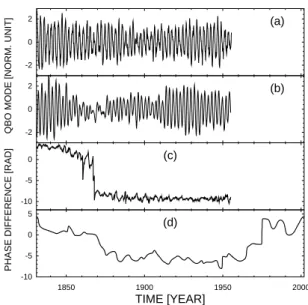
is clear and even the simultaneous statistical inference (see Paluˇs, 1995, and references therein) cannot jeopardize the significance of the results. The significant modes in the NAO are located at the frequencies (in cycles per month) 0.004, 0.006, 0.0104, 0.014, 0.037 and 0.049, corresponding to the periods of 240, 160, 96, 73, 27 and 20 months, respec-tively. Besides the zero frequency (trend) mode, the signifi-cant modes in the temperature are located at the frequencies 0.0104, 0.014, 0.016, 0.018, 0.025, 0.037 and 0.051, cor-responding to the periods of 96, 68, 64, 56, 40, 27 and 20 months, respectively. The modes with period 8 years were extracted and presented in Paluˇs and Novotn´a (2004), their mean frequency was estimated with higher precision as 7.8 years. Besides the latter modes (and the trend mode in the temperature), the highest regularity index was obtained for the modes with the period of 27 months (frequency 0.037). This frequency lies within the range of the quasi-biennial oscillations (QBO), therefore we will use the term “QBO modes”. The QBO modes were extracted from both the NAO index and the temperature, i.e., the raw data were projected on the related eigenvector, and are illustrated in Figs. 2a, b. The extracted modes are shorter than the original time series by the embedding dimension n=480 months, and there is an uncertainty of the exact timing of the modes equal to the em-bedding window of 40 years. We adjusted the temporal coor-dinate of the modes by maximizing their correlation with the original data, although this approach does not always give an unambiguous result.
5 Synchronization analysis: the method and results
Based on the concept of phase synchronization of chaotic oscillators (Rosenblum et al., 1996; Pikovsky et al., 2001), a novel technique has been developed to analyze complex, even non-stationary, bivariate data (Pikovsky et al., 2001; Paluˇs, 1997b). First, we calculate the instantaneous phases φ1(t )and φ2(t )of analyzed signals, in this case, of the QBO modes extracted from the NAO and the temperature data. The instantaneous phase and amplitude of a signal s(t ) can be determined by using the analytic signal concept of Gabor (1946), recently introduced into the field of nonlinear dynam-ics within the context of chaotic synchronization (Rosenblum et al., 1996). The analytic signal ψ (t) is a complex function of time defined as
ψ (t ) = s(t ) + j ˆs(t ) = A(t )ej φ (t ). (8) Usually, the imaginary part ˆs(t ) of the analytic signal ψ (t ) can be obtained by using the Hilbert transform of s(t)
ˆ s(t ) = 1 π P.V. Z ∞ −∞ s(τ ) t − τdτ. (9) 1850 1900 1950 2000 -10 -5 0 5 (d) TIME [YEAR]
PHASE DIFFERENCE [RAD]
-10 -5 0 (c) -2 0 2 (b)
QBO MODE [NORM. UNIT]
-2 0
2 (a)
Fig. 2. The QBO mode extracted from the monthly NAO index (a) and the monthly Prague near-surface air temperature series (b).
The instantaneous phase difference of the NAO and the temperature QBO modes obtained from the instantaneous phases computed from the SSA modes (c) and the same phase difference computed from the instantaneous phases estimated using the complex continuous wavelet transform (d).
(P.V. means that the integral is taken in the sense of the Cauchy principal value.) A(t ) is the instantaneous amplitude and the instantaneous phase φ (t ) of the signal s(t ) is φ (t ) =arctans(t )ˆ
s(t ). (10)
Having the analyzed signals extracted as the SSA modes, each oscillatory mode usually exists together with its orthog-onal (π/2-delayed or advanced) version. These two modes can be considered to be the real and imaginary parts of the analytic signal and the phase φ (t ) can be obtained according to Eq. (10). Another approach, also considered here, is based on the wavelet transform (Torrence and Compo, 1998). Ap-plying a continuous complex wavelet transform directly to the NAO index and the temperature time series, the complex coefficients related to the scale (frequency) of the studied cy-cles (the period of 27 months) can directly be used in Eq. (10) to estimate the phase φ (t ). Having the instantaneous phases φ1(t )and φ2(t )of the NAO and the temperature QBO modes, respectively, we define the instantaneous phase difference
1φ (t ) = φ1(t ) − φ2(t ). (11)
In the classical case of periodic self-sustained oscillators, phase synchronization is defined as phase locking, i.e., the phase difference is constant. In the case of phase-synchronized chaotic or other complex noisy systems, fluc-tuations of phase difference typically occur. Therefore, the criterion for phase synchronization is that the absolute val-ues of 1φ must be bounded (Rosenblum et al., 1996). When
1850 1900 1950 2000 -20 -10 0 10 20 (b) TIME [YEAR]
PHASE DIFFERENCE [RAD]
1850 1900 1950 2000 -20 -10 0 10 20 1850 1900 1950 2000 -20 -10 0 10 20 1850 1900 1950 2000 -20 -10 0 10 20 1850 1900 1950 2000 -20 -10 0 10 20 -20 0 20 40 60 (a) -20 0 20 40 60
Fig. 3. (a) The instantaneous phase difference of the NAO and the
temperature QBO modes obtained from the instantaneous phases computed from the SSA modes (thick solid line) compared with the instantaneous phase difference of the oscillatory modes of fre-quency 0.0407 (thin dashed line), again extracted by SSA from the monthly NAO index and the monthly Prague near-surface air tem-perature series. (b) The instantaneous phase difference of the NAO and the temperature QBO modes computed from the instantaneous phases estimated using the complex continuous wavelet transform (thick solid line) compared with the instantaneous phase differences computed in the same way, but with realization of the isospec-tral surrogate data used instead of the temperature time series (thin dashed/dotted lines).
the instantaneous phases are not represented as cyclic func-tions in the interval [0, 2π ] but as monotonously increasing functions on the whole real line, then the instantaneous phase difference 1φ (t ) is also defined on the real line and is an unbounded (increasing or decreasing) function of time for asynchronous states of systems, while epochs of phase syn-chronization appear as plateaus in the 1φ(t) vs. time plots. The phase difference 1φ(t ) of the NAO and the temperature QBO modes obtained from the instantaneous phases com-puted from the SSA modes as the real and the imaginary parts of the analytic signals is presented in Fig. 2c. After an initial decrease and a jump, there is a clear plateau start-ing at about the year 1870, extendstart-ing to 1955, when the SSA estimate of the phases ends due to the embedding dimension n=480 months. A larger part of the data can be exploited using the wavelet transform, which gives the phase differ-ence 1φ (t) of the NAO and the temperature QBO modes presented in Fig. 2d. Paluˇs et al. (2005) compared the three above mentioned methods for the estimation of instantaneous phase and demonstrated their equivalency. There are, how-ever, some differences in the numerical properties of the
es-timates. SSA uses the natural basis of the empirical orthog-onal functions and thus is more precise and sensitive to local extrema. Its drawback is the above mentioned uncertainty of the temporal localization of the modes and the phases. The cross-correlation method for the temporal localization does not always give unambiguous results and can hardly be fully automatized for the processing of large amounts of data. The wavelet method caused some smoothing of the estimates given by the shape of the wavelet basis functions leading to decreased precision of the estimates, however, the estimated phases are exactly localized in time and thus automated pro-cessing of large amounts of data is possible. Nevertheless, in the period 1870–1955, both methods consistently estimate the plateau in the 1φ (t ) vs. time plot, i.e. they indicate phase synchronization between the QBO modes in the NAO and in the temperature. The flatness of the plateau in the 1φ (t ) vs. time plot is indeed visually convincing, demonstrating the bounded character of 1φ (t ). One can doubt, however, whether this is indeed a demonstration of the physical phe-nomenon of phase synchronization. The extraction of the SSA modes is in fact a very narrow band filtration of the analyzed signal. Two sine waves with the same frequency would be formally phase-locked without any physical inter-action. In order to demonstrate that the plateau in Figs. 1c, d is not a trivial consequence of the filtration, we compute the instantaneous phase difference for two SSA modes of close frequency. The modes on the frequency 0.0407 in both the NAO and the temperature series (Fig. 1) are not significant in our enhanced MC SSA test and thus do not represent any physically existing oscillation but just the narrow-band filtra-tion of the background noise. Their phase difference (Fig. 3a, thin dashed line) behaves as an unbounded random walk.
We can go further and compute the instantaneous phase difference of oscillatory modes on the same frequency (pe-riod 27 months) using the wavelet method applied to the NAO index, but instead of the temperature data we use so-called isospectral surrogate data (Theiler et al., 1992; Paluˇs, 1995). In the above MC SSA, we used the AR(1) model as the surrogate data which preserved the 1/f character of the spectrum of the data but not possible cycles. In this case, we need to preserve the possible existence of cycles, i.e., we need to preserve the whole spectrum of the signal, but to randomize phases of such cycles in order to destroy any de-pendence on the NAO possibly contained in the temperature data. The isospectral surrogate data are constructed from the real temperature data by means of the Fast Fourier Transform (FFT): The FFT is computed, the magnitude of the FFT coef-ficients (i.e. the power spectrum) is preserved, but the Fourier phases are randomized. After inverse FFT, we obtain a sig-nal with the same power spectrum as the temperature series, but independent of the NAO or any other real atmospheric process.
The instantaneous phase differences 1φ (t ) obtained us-ing four different (independently randomized) realizations of the isospectral surrogate data are presented in Fig. 3b as thin
M. Paluˇs and D. Novotn´a: Phase-synchronized QBO in the NAO and temperature records 293 dashed and/or dotted lines. They are apparently unbounded,
they look smoother due to their estimation by means of the wavelet transform.
We will not rely on the above visual evidence but will prove the existence of phase synchronization in a statistical way. First, we express the flatness of the plateau in the 1φ (t ) vs. time plot in a quantitative way. Now, we consider 1φ (t ) as 1φ (t) mod(2π ) and use a simple trigonometric statistic, known also as the mean resultant length (MRL) (Allefeld and Kurths, 2004):
MRL = q
hcos(1φ(t))i2+ hsin(1φ (t))i2 (12) where hi means the temporal average. The MRL tends to zero for asynchronous processes and to one for phase locked sys-tems. Considering real noisy data, neither 0 nor 1 is reached, but we can expect that the MRL for synchronized oscillations will be significantly larger than for unsynchronized (surro-gate) processes.
Paluˇs (1997b) demonstrated that the instantaneous phases φ1, φ2of phase-synchronized systems are confined in strip-like structures when plotted in the plane (0, 2π )×(0, 2π ), while the instantaneous phases φ1, φ2of asynchronous pro-cesses almost homogeneously fill the plane (0, 2π )×(0, 2π ). The dependence between φ1and φ2, i.e., the structure in the φ1, φ2plot, can be quantified by using various statistical or information-theoretic approaches. Here we use the mutual information (Cover and Thomas, 1991), defined as
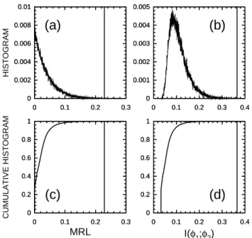
I (φ1, φ2) = Z 2π 0 Z 2π 0 p1,2(φ1, φ2)log p1,2(φ1, φ2) p1(φ1)p2(φ2) dφ1dφ2, (13) where p1(φ1)and p2(φ2)are probability distributions of the phases φ1and φ2, respectively, and p1,2(φ1, φ2)is their joint distribution. Theoretically, independence of the phases, i.e., the absence of phase synchronization, means homogeneous distribution of the points (φ1, φ2)and I (φ1, φ2)=0; while for phase synchronization, i.e., a mutual dependence of the phases, I (φ1, φ2)>0 holds. For reliable detection of the phase synchronization in experimental data, it is necessary to establish that I (φ1, φ2)>0 with a statistical significance. Therefore, we compute both the MRL and I (φ1, φ2)for a large number (5000) of realizations of the surrogate data, construct histograms and cumulative histograms of the MRL and I (φ1, φ2)surrogate distributions (Fig. 4) and compare them with the MRL and I (φ1, φ2)values obtained for the NAO and temperature data (solid vertical lines in Fig. 4). The cumulative histograms can be used for estimation of the significance of the test – the p value which is in fact the probability, that such a value of the MRL or I (φ1, φ2), as obtained from the NAO and temperature data, can be ob-tained by chance from unsynchronized or independent pro-cesses with the same frequency spectra. The obtained values
Paluˇs & Novotn´a: Phase-synchronized QBO in the NAO and temperature records 7
0 0.1 0.2 0.3 0 0.2 0.4 0.6 0.8 1
(c)
MRL CUMULATIVE HISTOGRAM 0 0.1 0.2 0.3 0 0.2 0.4 0.6 0.8 1 0 0.1 0.2 0.3 0.4 0 0.2 0.4 0.6 0.8 1(d)
I(φ1;φ2) 0 0.1 0.2 0.3 0.4 0 0.2 0.4 0.6 0.8 1 0 0.1 0.2 0.3 0 0.002 0.004 0.006 0.008 0.01(a)
HISTOGRAM 0 0.1 0.2 0.3 0 0.002 0.004 0.006 0.008 0.01 0 0.1 0.2 0.3 0.4 0 0.001 0.002 0.003 0.004 0.005(b)
0 0.1 0.2 0.3 0.4 0 0.001 0.002 0.003 0.004 0.005Fig. 4. Histograms (a,b) and cumulative histograms (c,d) for the surrogate distribution of the mean resultant length (a,c) and the mu-tual information I(φ1, φ2) (b,c). The related values obtained from
the QBO phases extracted from the monthly NAO index and the monthly Prague near-surface air temperature series are presented as the solid vertical lines. The wavelet transform was used for the phase estimation.
like structures when plotted in the plane (0, 2π) × (0, 2π), while the instantaneous phases φ1, φ2of asynchronous pro-cesses almost homogeneously fill the plane (0, 2π)×(0, 2π). The dependence between φ1and φ2, i.e., the structure in the φ1, φ2plot, can be quantified by using various statistical or information-theoretic approaches. Here we use the mutual information (Cover & Thomas, 1991), defined as
I(φ1, φ2) = Z 2π 0 Z 2π 0 p1,2(φ1, φ2) log p1,2(φ1, φ2) p1(φ1)p2(φ2)dφ1dφ2, (13) where p1(φ1) and p2(φ2) are probability distributions of the phases φ1and φ2, respectively, and p1,2(φ1, φ2) is their joint distribution. Theoretically, independence of the phases, i.e., the absence of phase synchronization, means homogeneous distribution of the points (φ1, φ2) and I(φ1, φ2) = 0; while for phase synchronization, i.e., a mutual dependence of the phases, I(φ1, φ2) > 0 holds. For reliable detection of the phase synchronization in experimental data, it is necessary to establish that I(φ1, φ2) > 0 with a statistical significance. Therefore, we compute both the MRL and I(φ1, φ2) for a large number (5,000) of realizations of the surrogate data, construct histograms and cumulative histograms of the MRL and I(φ1, φ2) surrogate distributions (Fig. 4) and compare them with the MRL and I(φ1, φ2) values obtained for the NAO and temperature data (solid vertical lines in Fig. 4). The cumulative histograms can be used for estimation of the significance of the test – the p value which is in fact the
0 0.1 0.2 0.3 0 0.2 0.4 0.6 0.8 1
(c)
MRL CUMULATIVE HISTOGRAM 0 0.1 0.2 0.3 0 0.2 0.4 0.6 0.8 1 0 0.1 0.2 0.3 0.4 0 0.2 0.4 0.6 0.8 1(d)
I(φ1;φ2) 0 0.1 0.2 0.3 0.4 0 0.2 0.4 0.6 0.8 1 0 0.1 0.2 0.3 0 0.001 0.002 0.003 0.004 0.005(a)
HISTOGRAM 0 0.1 0.2 0.3 0 0.001 0.002 0.003 0.004 0.005 0 0.1 0.2 0.3 0.4 0 0.001 0.002 0.003 0.004 0.005(b)
0 0.1 0.2 0.3 0.4 0 0.001 0.002 0.003 0.004 0.005Fig. 5. Histograms (a,b) and cumulative histograms (c,d) for the distribution of the mean resultant length (a,c) and the mutual infor-mation I(φ1, φ2) (b,c) obtained from the bivariate surrogate data
preserving the crosscorrelation between the NAO and temperature series. The related values obtained from the QBO phases extracted from the monthly NAO index and the monthly Prague near-surface air temperature series are presented as the solid vertical lines. The wavelet transform was used for the phase estimation.
probability, that such a value of the MRL or I(φ1, φ2), as obtained from the NAO and temperature data, can be ob-tained by chance from unsynchronized or independent pro-cesses with the same frequency spectra. The obtained val-ues are p < 0.0005 for the MRL and p < 0.00002 for the I(φ1, φ2) test. We can conclude that phase synchronization of the NAO and temperature QBO modes has been proven with a high statistical significance.
6 Discussion of results
An introduction of relatively new, nonlinear methods to anal-ysis of experimental time series always evokes two types of questions: 1) Does the new method bring more infor-mation than common, already verified linear methods? 2) Does the the new nonlinear method indeed reflect a nonlin-ear phenomenon or is a linnonlin-ear model/explanation sufficient? In this case, cannot a simple cross-correlation mimic the phe-nomenon of phase synchronization? Searching for answers to both questions, we perform the same testing as above (Fig. 4), but instead of (independent) surrogate data which preserved spectral properties of individual time series, now we construct bivariate surrogate data (Prichard & Theiler, 1994; Paluˇs, 1996b) preserving also the cross-correlations of the original (NAO and temperature) time series. Looking at the resulting histograms (Fig. 5) we can see that bivariate FFT surrogate data can reject the null hypothesis of inde-pendence used in the previous test (Fig. 4) and, indeed, even Fig. 4. Histograms (a, b) and cumulative histograms (c, d) for the
surrogate distribution of the mean resultant length (a, c) and the
mu-tual information I (φ1, φ2)(b, c). The related values obtained from
the QBO phases extracted from the monthly NAO index and the monthly Prague near-surface air temperature series are presented as the solid vertical lines. The wavelet transform was used for the phase estimation.
are p<0.0005 for the MRL and p<0.00002 for the I (φ1, φ2) test. We can conclude that phase synchronization of the NAO and temperature QBO modes has been proven with a high statistical significance.
6 Discussion of results
An introduction of relatively new, nonlinear methods to anal-ysis of experimental time series always evokes two types of questions: 1) Does the new method bring more infor-mation than common, already verified linear methods? 2) Does the the new nonlinear method indeed reflect a nonlin-ear phenomenon or is a linnonlin-ear model/explanation sufficient? In this case, cannot a simple cross-correlation mimic the phe-nomenon of phase synchronization? Searching for answers to both questions, we perform the same testing as above (Fig. 4), but instead of (independent) surrogate data which preserved spectral properties of individual time series, now we construct bivariate surrogate data (Prichard and Theiler, 1994; Paluˇs, 1996b) preserving also the cross-correlations of the original (NAO and temperature) time series. Look-ing at the resultLook-ing histograms (Fig. 5) we can see that bi-variate FFT surrogate data can reject the null hypothesis of independence used in the previous test (Fig. 4) and, indeed, even cross-correlated linear processes could be erroneously considered as phase-synchronized nonlinear oscillations. In
0 0.1 0.2 0.3 0 0.2 0.4 0.6 0.8 1
(c)
MRL CUMULATIVE HISTOGRAM 0 0.1 0.2 0.3 0 0.2 0.4 0.6 0.8 1 0 0.1 0.2 0.3 0.4 0 0.2 0.4 0.6 0.8 1(d)
I(φ1;φ2) 0 0.1 0.2 0.3 0.4 0 0.2 0.4 0.6 0.8 1 0 0.1 0.2 0.3 0 0.002 0.004 0.006 0.008 0.01(a)
HISTOGRAM 0 0.1 0.2 0.3 0 0.002 0.004 0.006 0.008 0.01 0 0.1 0.2 0.3 0.4 0 0.001 0.002 0.003 0.004 0.005(b)
0 0.1 0.2 0.3 0.4 0 0.001 0.002 0.003 0.004 0.005Fig. 4. Histograms (a,b) and cumulative histograms (c,d) for the surrogate distribution of the mean resultant length (a,c) and the mu-tual information I(φ1, φ2) (b,c). The related values obtained from the QBO phases extracted from the monthly NAO index and the monthly Prague near-surface air temperature series are presented as the solid vertical lines. The wavelet transform was used for the phase estimation.
like structures when plotted in the plane (0, 2π) × (0, 2π), while the instantaneous phases φ1, φ2 of asynchronous pro-cesses almost homogeneously fill the plane (0, 2π)×(0, 2π). The dependence between φ1and φ2, i.e., the structure in the φ1, φ2plot, can be quantified by using various statistical or information-theoretic approaches. Here we use the mutual information (Cover & Thomas, 1991), defined as
I(φ1, φ2) = Z 2π 0 Z 2π 0 p1,2(φ1, φ2) log p1,2(φ1, φ2) p1(φ1)p2(φ2)dφ1dφ2, (13) where p1(φ1) and p2(φ2) are probability distributions of the phases φ1and φ2, respectively, and p1,2(φ1, φ2) is their joint distribution. Theoretically, independence of the phases, i.e., the absence of phase synchronization, means homogeneous distribution of the points (φ1, φ2) and I(φ1, φ2) = 0; while for phase synchronization, i.e., a mutual dependence of the phases, I(φ1, φ2) > 0 holds. For reliable detection of the phase synchronization in experimental data, it is necessary to establish that I(φ1, φ2) > 0 with a statistical significance. Therefore, we compute both the MRL and I(φ1, φ2) for a large number (5,000) of realizations of the surrogate data, construct histograms and cumulative histograms of the MRL and I(φ1, φ2) surrogate distributions (Fig. 4) and compare them with the MRL and I(φ1, φ2) values obtained for the NAO and temperature data (solid vertical lines in Fig. 4).
0 0.1 0.2 0.3 0 0.2 0.4 0.6 0.8 1
(c)
MRL CUMULATIVE HISTOGRAM 0 0.1 0.2 0.3 0 0.2 0.4 0.6 0.8 1 0 0.1 0.2 0.3 0.4 0 0.2 0.4 0.6 0.8 1(d)
I(φ1;φ2) 0 0.1 0.2 0.3 0.4 0 0.2 0.4 0.6 0.8 1 0 0.1 0.2 0.3 0 0.001 0.002 0.003 0.004 0.005(a)
HISTOGRAM 0 0.1 0.2 0.3 0 0.001 0.002 0.003 0.004 0.005 0 0.1 0.2 0.3 0.4 0 0.001 0.002 0.003 0.004 0.005(b)
0 0.1 0.2 0.3 0.4 0 0.001 0.002 0.003 0.004 0.005Fig. 5. Histograms (a,b) and cumulative histograms (c,d) for the distribution of the mean resultant length (a,c) and the mutual infor-mation I(φ1, φ2) (b,c) obtained from the bivariate surrogate data preserving the crosscorrelation between the NAO and temperature series. The related values obtained from the QBO phases extracted from the monthly NAO index and the monthly Prague near-surface air temperature series are presented as the solid vertical lines. The wavelet transform was used for the phase estimation.
probability, that such a value of the MRL or I(φ1, φ2), as obtained from the NAO and temperature data, can be ob-tained by chance from unsynchronized or independent pro-cesses with the same frequency spectra. The obtained val-ues are p < 0.0005 for the MRL and p < 0.00002 for the I(φ1, φ2) test. We can conclude that phase synchronization of the NAO and temperature QBO modes has been proven with a high statistical significance.
6 Discussion of results
An introduction of relatively new, nonlinear methods to anal-ysis of experimental time series always evokes two types of questions: 1) Does the new method bring more infor-mation than common, already verified linear methods? 2) Does the the new nonlinear method indeed reflect a nonlin-ear phenomenon or is a linnonlin-ear model/explanation sufficient? In this case, cannot a simple cross-correlation mimic the phe-nomenon of phase synchronization? Searching for answers to both questions, we perform the same testing as above (Fig. 4), but instead of (independent) surrogate data which preserved spectral properties of individual time series, now we construct bivariate surrogate data (Prichard & Theiler, 1994; Paluˇs, 1996b) preserving also the cross-correlations of the original (NAO and temperature) time series. Looking at the resulting histograms (Fig. 5) we can see that bivariate Fig. 5. Histograms (a, b) and cumulative histograms (c, d) for the
distribution of the mean resultant length (a, c) and the mutual
infor-mation I (φ1, φ2)(b, c) obtained from the bivariate surrogate data
preserving the crosscorrelation between the NAO and temperature series. The related values obtained from the QBO phases extracted from the monthly NAO index and the monthly Prague near-surface air temperature series are presented as the solid vertical lines. The wavelet transform was used for the phase estimation.
our case, however, the values of the mean resultant length and the mutual information I (φ1, φ2)show that the associa-tion of the phases of the QBO modes in the NAO and tem-perature data is still significantly stronger that that obtained from bivariate surrogate data. The obtained significance val-ues are p<0.02 for the MRL and p<0.008 for the I (φ1, φ2) test (Fig. 5). So we can conclude that we have detected a nonlinear interaction of the QBO modes in the NAO and tem-perature records which neither can be explained by a linear model, nor can be sufficiently described by linear measures. On the other hand, the question whether we have detected the phase synchronization sensu stricto is more subtle. Phase synchronization is a phenomenon occurring in an interaction of two autonomous (possibly chaotic and/or noisy) oscilla-tory processes. The atmospheric temperature and pressure (giving the NAO index) are two variables of one large non-linear spatio-temporal system – the atmosphere. It is a ques-tion of the level of descripques-tion and/or approximaques-tion whether some modes of atmospheric variability can or cannot be con-sidered as autonomous processes interacting through a non-linear and time variable coupling. It is known that the re-lationship between the NAO and the NHT is time-variable (Polyakova et al., 2006) and can be influenced by solar (Gi-meno et al., 2003) and geomagnetic activity (Bochn´ıˇcek and Hejda, 2005). The term dynamics reflected in
long-range correlations or long-term memory have different prop-erties in the NAO and in the temperature records (Fraedrich, 2003). Recently, Mokhov and Smirnov (2006) have demon-strated that the NAO interacts, or is influenced by the other global atmospheric oscillatory process – the El Ni˜no South-ern Oscillation. We believe that phase synchronization can be at least a good working model and the above utilized tools can be developed in the context of phase synchronization to measure the association of phases. We also believe that mea-sures characterizing the coupling direction (causality) in the interaction of phases (Rosenblum and Pikovsky, 2001; Paluˇs and Stefanovska, 2003) can help in the understanding of the interaction of modes of atmospheric variability (Mokhov and Smirnov, 2006). This does not mean that, in particular stud-ies, the new, nonlinear methods should not be accompanied by standard approaches and their extensions, especially by those that can cope with nonstationarity, e.g. cross-wavelet or wavelet coherence approaches (Grinsted et al., 2004; Ma-raun and Kurths, 2004).
7 Conclusions
In this paper, we demonstrate a sophisticated combination of methods from nonlinear dynamics with an established linear method in an application to multivariate geophysical data. Monte Carlo Singular System Analysis has been extended by evaluating and testing the regularity of the dynamics of the SSA modes against the colored noise null hypothesis in addition to the test based on variance (eigenvalues). The non-linear approach to the measurement of regularity and pre-dictability of the dynamics, based on a coarse-grained es-timate of the mutual information, increases the MC SSA test sensitivity and reliability in the detection of dynamical modes which are relatively more regular than those obtained by decomposition of colored noise.
Enhanced MC SSA has been applied to records of monthly average near-surface air temperature from several European locations as well as to the monthly NAO index and several significant oscillatory modes have been detected by testing the regularity of the modes. Then, we focused on the oscilla-tory modes with the average period 27 months which can be considered as realizations of the quasi-biennial oscilla-tions (QBO) in both the NAO index and temperature data. Another method from nonlinear dynamics, synchronization analysis (Pikovsky et al., 2001; Paluˇs, 1997b) gives the pos-sibility to establish existence of coupling between the QBO modes present in the NAO and in the temperature time series. Applying the concept of surrogate data, we proved with high statistical significance that the QBO modes in the NAO and in the temperature time series are phase synchronized. We also showed that the phenomenon of phase synchronization is probably a real physical phenomenon and its signatures do not occur in phase relations of formally extracted, non sig-nificant SSA modes, although they represent a very
narrow-M. Paluˇs and D. Novotn´a: Phase-synchronized QBO in the NAO and temperature records 295 band filtered colored noise which could erroneously be
con-sidered as real oscillations. The statistical evidence for the phase synchronization between the QBO modes can be con-sidered as additional evidence for the real existence of these oscillatory modes in the dynamics of NAO and air temper-ature and thus, in return, it confirms the validity of our en-hanced MC SSA test.
The introduced set of methods will be applied to tempera-ture data from other stations, as well as to other meteorologi-cal measurements and to the NCEP/NCAR reanalysis series. We believe that the results will help us to understand how global atmospheric circulation processes influence European weather and climate changes on various temporal scales.
Acknowledgements. This study is supported by the Grant Agency of the Academy of Sciences of the Czech Republic, project No. IAA3042401, and in part by the Institutional Research Plans AV0Z10300504 and AV0Z30420517.
Edited by: M. Thiel Reviewed by: two referees
References
Allefeld, C. and Kurths, J.: Testing for phase synchronization, Int. J. Bif. Chaos, 14(2), 406–416, 2004.
Allen, M. R. and Smith, L. A.: Investigating the origins and signif-icance of low-frequency modes of climate variability, Geophys. Res. Lett. 21, 883–886, 1994.
Allen, M. R. and Smith, L. A.: Monte Carlo SSA: Detecting ir-regular oscillations in the presence of colored noise, J. Climate, 9(12), 3373–3404, 1996.
Bochn´ıˇcek, J. and Hejda, P.: The winter NAO pattern changes in association with solar and geomagnetic activity, J. Atmos. Solar-Terrestrial Phys., 67, 17–32, 2005.
Bojariu, R. and Gimeno, L.: Predictability and numerical modelling of the North Atlantic Oscillation, Earth-Sci. Rev., 63(1–2), 145– 168, 2003.
Cover, T. M. and Thomas, J. A.: Elements of Information Theory, J. Wiley & Sons, New York, 1991.
Eden, C., Greatbatch, R. J., and Lu, J.: Prospects for decadal pre-diction of the North Atlantic Oscillation (NAO), Geophys. Res. Lett., 29(10), 1466–1469, 2002.
Fernandez, I., Hernandez, C. N., and Pacheco, J. M.: Is the North Atlantic Oscillation just a pink noise? Physica A, 323, 705–714, 2003.
Fraedrich, K.: Short- and long term memory of the atmosphere, in: Chaos in Geophysical Flows, edited by: Boffetta, G., Larcotta, S., Visconti G., and Vulpiani, A., Otto Editore, Torino, 63–104, 2003.
Gabor, D.: Theory of Communication, J. IEE London, 93, 429–457, 1946.
G´amiz-Fortis, S. R., Pozo-V´azques, D., Esteban-Parra, M. J., and Castro-D´ıez, Y.: Spectral characteristics and predictability of the NAO assessed through Singular Spectral Analysis, J. Geophys. Res., 107(D23), 4685, 2002.
Gao, J. B., Cao, Y., and Lee, J.-M.: Principal component analysis
of 1/fαnoise, Phys. Lett. A, 314, 392–400, 2003.
Ghil, M. and Vautard, R.: Interdecadal oscillations and the warming trend in global temperature time series, Nature, 350(6316), 324– 327, 1991.
Gimeno, L., de la Torre, L., Nieto, R., Garc´ıa, R., Hern´andez, E., and Ribera, P.: Changes in the relationship NAO–Northern hemi-sphere temperature due to solar activity, Earth Planet. Sci. Lett., 206, 15–20, 2003.
Grinsted A., Moore, J. C., and Jevrejeva, S.: Application of the cross wavelet transform and wavelet coherence to geophysical time series, Nonlin. Processes Geophys., 11, 561–566, 2004, http://www.nonlin-processes-geophys.net/11/561/2004/. Hurrell, J. W., Kushnir, Y., and Visbeck, M.: Climate – The North
Atlantic oscillation, Science, 291(5504), 603, 2001.
Keppenne, C. L. and Ghil, M.: Adaptive filtering and the Southern Oscillation Index, J. Geophys. Res., 97, 20 449–20 454, 1992. Maraun, D. and Kurths, J.: Cross wavelet analysis: significance
testing and pitfalls, Nonlin. Processes Geophys., 11, 505–514, 2004,
http://www.nonlin-processes-geophys.net/11/505/2004/. Mokhov, I. I. and Smirnov, D. A.: El Ni˜no-Southern Oscillation
drives North Atlantic Oscillation as revealed with nonlinear tech-niques from climatic indices, Geophys. Res. Lett., 33, L03708, doi:10.1029/2005GL024557, 2006.
Paluˇs, M.: Testing for nonlinearity using redundancies: Quantita-tive and qualitaQuantita-tive aspects, Physica D, 80, 186–205, 1995. Paluˇs, M.: Coarse-grained entropy rates for characterization of
complex time series, Physica D, 93, 64–77, 1996a.
Paluˇs, M.: Detecting nonlinearity in multivariate time series, Phys. Lett. A, 213, 138–147, 1996b.
Paluˇs, M.: Kolmogorov entropy from time series using information-theoretic functionals, Neural Network World, (http://www.uivt.
cas.cz/∼mp/papers/rd1a.ps), 3/97, 269–292, 1997a.
Paluˇs, M.: Detecting phase synchronization in noisy systems, Phys. Lett. A, 235, 341–351, 1997b.
Paluˇs, M. and Novotn´a, D.: Detecting modes with nontrivial dy-namics embedded in colored noise: Enhanced Monte Carlo SSA and the case of climate oscillations, Phys. Lett. A, 248, 191–202, 1998.
Paluˇs, M. and Stefanovska, A.: Direction of coupling from phases of interacting oscillators: An information-theoretic approach, Phys. Rev. E, 67, 055201(R), 2003.
Paluˇs, M. and Novotn´a, D.: Enhanced Monte Carlo Singular Sys-tem Analysis and detection of period 7.8 years oscillatory modes in the monthly NAO index and temperature records, Nonlin. Pro-cesses Geophys., 11, 721–729, 2004,
http://www.nonlin-processes-geophys.net/11/721/2004/. Paluˇs, M., Novotn´a, D., and Tichavsk´y, P.: Shifts of seasons at
the European mid-latitudes: Natural fluctuations correlated with the North Atlantic Oscillation, Geophys. Res. Lett., 32, L12805, doi:10.1029/2005GL022838, 2005.
Pikovsky, A., Rosenblum, M., and Kurths, J.: Synchronization. A Universal Concept in Nonlinear Sciences, Cambridge University Press, 2001.
Polyakova, E. I., Journel, A. G., Polyakov, I. V., and Bhatt, U. S.: Changing relationship between the North Atlantic Oscilla-tion and key North Atlantic climate parameters, Geophys. Res. Lett., 33, L03711, doi:10.1029/2005GL024573, 2006.
Pozo-V´azques, D., Esteban-Parra, M. J., Rodrigo, F. S., and Castro-D´ıez, Y.: A study of NAO variability and its possible nonlinear influence on European surface temperature, Clim. Dyn., 17, 701– 715, 2001.
Press, W. H., Flannery, B. P., Teukolsky, S. A., and Vetterling, W. T.: Numerical Recipes: The Art of Scientific Computing. Cam-bridge Univ. Press, CamCam-bridge, 1986.
Prichard, D. and Theiler, J.: Generating surrogate data with several simultaneously measured variables, Phys. Rev. Lett., 73, 951-954, 1994.
Rosenblum, M. G., Pikovsky, A. S., and Kurths, J.: Phase synchro-nization of chaotic oscillators, Phys. Rev. Lett., 76, 1804–1807, 1996.
Rosenblum, M. G. and Pikovsky, A. S.: Detecting direction of coupling in interacting oscillators, Phys. Rev. E, 64, 045202(R), 2001.
Theiler, J., Eubank, S., Longtin, A., Galdrikian, B., and Farmer, J. D.: Testing for nonlinearity in time series: the method of surro-gate data, Physica D, 58, 77–94, 1992.
Torrence, C. and Compo, G. P.: A practical guide to wavelet analy-sis, Bull. Amer. Meteorol. Soc., 79(1), 61–78, 1998.
Vautard, R. and Ghil, M.: Singular spectrum analysis in nonlinear dynamics, with applications to paleoclimatic time series, Physica D, 35, 395–424, 1989.
Vautard, R., Yiou, P., and Ghil, M.: Singular spectrum analysis: a toolkit for short noisy chaotic signals, Physica D, 58, 95–126, 1992.
Yiou, P., Ghil, M., Jouyel, J., Paillard, D., and Vautard, R.: Nonlin-ear variability of the climatic system, from singular and power spectra of Late Quarternary records, Clim. Dyn., 9, 371–389, 1994.