HAL Id: hal-03006522
https://hal.archives-ouvertes.fr/hal-03006522
Submitted on 19 Nov 2020
HAL is a multi-disciplinary open access
archive for the deposit and dissemination of sci-entific research documents, whether they are pub-lished or not. The documents may come from teaching and research institutions in France or abroad, or from public or private research centers.
L’archive ouverte pluridisciplinaire HAL, est destinée au dépôt et à la diffusion de documents scientifiques de niveau recherche, publiés ou non, émanant des établissements d’enseignement et de recherche français ou étrangers, des laboratoires publics ou privés.
To cite this version:
Eric Debayle, Thomas Bodin, Stéphanie Durand, Yanick Ricard. Seismic evidence for partial melt be-low tectonic plates. Nature, Nature Publishing Group, 2020, 586 (7830), pp.555-559. �10.1038/s41586-020-2809-4�. �hal-03006522�
Seismic evidence for partial melt below tectonic plates
1Eric Debayle1, Thomas Bodin1, Stéphanie Durand1 and Yanick Ricard2 2 1Univ Lyon, Univ Lyon 1, ENSL, CNRS, LGL-TPE, F-69622, Villeurbanne, France 3 2Univ Lyon, ENSL, Univ Lyon 1, CNRS, LGL-TPE, F-69007, Lyon, France 4 5
The seismic low velocity zone (LVZ) of the upper mantle is generally 6
associated with a low-viscosity asthenosphere that plays a key role for the 7
dynamics of plate tectonics1. However, its origin remains enigmatic, some 8
authors attributing the reduction in seismic velocity to a small amount of 9
partial melt2,3, others invoking solid-state mechanisms near the solidus4–6, or 10
the effect of volatile contents6. Observations of shear attenuation provide 11
additional constraints to unravel the origin of the LVZ7. Here, we report the 12
discovery of partial melt within the LVZ from the simultaneous 13
interpretation of global 3D shear attenuation and velocity models. We 14
observe that partial melting down to 150-200 km depth beneath mid-ocean 15
ridges, major hotspots and back-arc regions feeds the asthenosphere. A small 16
part of this melt (<0.30%) remains trapped within the oceanic LVZ. The 17
amount of melt is related to plate velocities and increases significantly 18
between 3 and 5 cm yr-1, similar to previous observations of mantle crystal 19
alignement underneath tectonic plates8. Our observations suggest that by 20
reducing viscosity9, melt facilitates plate motion and large-scale crystal 21
alignment in the asthenosphere. Melt is absent under most of the continents. 22
Our finding results from the simultaneous analysis of two upper mantle 23
tomographic models of shear wave velocity (Vs) and attenuation (parameterised 24
with Qs the quality factor, a measure of energy dissipation). Until now, most global 25 tomographic studies of the upper mantle and their thermochemical interpretation 26 have focused on shear velocity4,7. Recent experiments on olivine suggest that wave 27 speed and attenuation are insensitive to water, which would imply that elevated 28
water contents are not responsible for the LVZ10. However, Vs is sensitive to 29
temperature, composition and melt content, and deciphering the causes of its 30
variations represents a strongly non-unique inverse problem, severely limiting our 31
understanding of the Earth's interior. Shear attenuation has a different sensitivity 32
to these quantities, and therefore provides complementary constraints on the 33
origin of seismic heterogeneities11. Shear attenuation is negligibly dependent on 34
major element chemistry12, and exponentially dependent on temperature13. The 35 relation between attenuation and melt is debated, with some authors arguing for a 36 weak dependence based on experiments, models and seismological observations12, 37 while others suggest a larger effect3. Measuring shear attenuation is nevertheless 38 difficult. For this reason, only a few global Qs models have been published in the 39
last 20 years14, and the only recent joint interpretation of 3D Qs and Vs 40
tomographic models at global scale is based on models built from different 41 datasets and modeling approaches15. 42 The novelty of our study is to simultaneously interpret two recent global Vs and Qs 43 models that are consistent as obtained from the same Rayleigh wave dataset, at the 44 same resolution and using the same modelling approach. These Vs (DR2020s) and 45
Qs (QsASR17) models are displayed in Figure 1. Details of our tomographic 46
procedure can be found in Methods. Before interpreting these two models in the 47
light of laboratory experiments, a few words are needed to emphasize in what 48
temperature and pressure range our interpretation is pertinent. The attenuation 49
models derived by mineral physicists4,13 are valid for temperatures T larger than 50
900°C, which correspond to the base of the lithosphere and to the asthenosphere. 51
They consider thermally activated processes varying exponentially with 1/T that 52
would imply quality factor in excess of 2,000 in the upper 100 km of the 53
lithosphere and reaching several million near the surface (see Methods). However, 54
finite Qs is observed in the crust and in the cold mantle lithosphere where 55 attenuation is most likely related to non-thermal processes such as scattering or 56 fluid-fracture interactions14. Furthermore, the attenuation observed in seismology 57 accumulates along the seismic ray and the observation of Qs is only possible when 58 the amplitude of a wave is measurably smaller than in a pure elastic model. Given 59
the uncertainties on amplitude data, it appears impossible to resolve quality 60
factors larger than ~2,000 with long period Rayleigh waves (at periods of 100s, 61
assuming velocities of 4.5 km s-1 and ray lengths of 10,000 km, the amplitude 62
reduction with respect to a pure elastic model, would be less than 3.5%). Our 63
inversion leads indeed to a Qs model with strong lateral variations, by two orders 64
of magnitudes, but with a maximum Qs of ~1,750. Our attenuation model is 65
therefore mostly adapted to depths greater or equal to ~100 km, where Qs values 66
between fifty and a few hundreds are expected15. Therefore, our interpretation 67
applies to the oceanic asthenosphere and the mantle structure at depths greater or 68
equal to ~100 km, where our tomographic models are acurate and where 69
conditions similar to those used in laboratory experiments prevail. 70
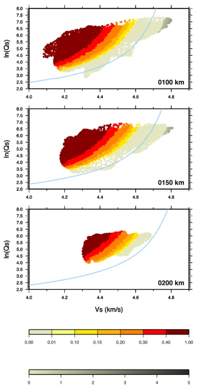
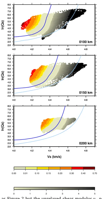
Figure 2 displays Qs as a function of Vs for each pixel of the maps, at different 71
depths in the upper mantle. The curves in dark and light blue represent the 72
theoretical relations due to temperature variations for a meltless pyrolitic 73
mantle16, given by two anelasticity models4,13 based on laboratory experiments, 74
appropriate for asthenospheric conditions (see Methods for details). These models 75
only explain a limited part of the velocities and attenuations of our dataset. We 76
consider that the first theoretical curve4 is compatible with a given Vs-Qs 77
observation if it falls within the typical uncertainties of the Vs and ln(Qs) 78
observations, 1% and 10% respectively (ivory colour). We show in Methods and 79
supplementary Figures S1-10 that reconciling the low values of Vs with Qs cannot 80
be done by invoking radial anisotropy, elastically accomodated grain boundary 81
sliding, or the effect of composition or water. However, this can be done by adding 82
partial melt, thus reducing Vs, and shifting the theoretical curves to the left in 83
Figure 2, since as discussed below, adding partial melt reduces Vs but has little effect 84
on Qs. Warm colours in Figure 2 indicate the amount of melt (<0.7%) needed to 85
reconcile observations with the first theoretical model4 (dark blue curve), which 86
requires the smallest amount of melt. On the right side of the ivory region, points in 87 grey are those for which Vs is too high compared to the theoretical value. They are 88 associated with the lithospheric depletion of cratonic roots. In this case, the grey 89 intensity quantifies the departure in percent from the theoretical curve assuming a 90 meltless pyrolitic mantle. Results using the second theoretical model13 are shown 91
in Figures S11-12. They lead essentially to the same conclusions, but require 92 larger melt fractions (up to 1%), which are more difficult to reconcile with the very 93 small melt fraction (~0.1%) suggested by geochemical studies4. 94 The effect of melt on Vs has been estimated to 7.9% reduction per percent of melt 95
based on model calculations17. Recent experiments3 are in qualitative agreement 96
but require a slightly larger Vs reduction (Figure S13). The effect of melt on 97
attenuation is not well constrained and depends on the mechanisms of 98
attenuation. We show in Methods that melt may have a large effect on Qs at short 99
period (1 s), but not in the period range of surface waves (50-250s). We therefore 100
neglect the effect of melt on Qs and we model its effect on Vs based on recent 101
experiments3. Figure 2 shows that the slowest shear velocities require less than 102
0.7 % of melt. 103
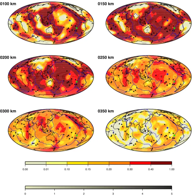
Figure 3 displays global maps of melt content at different depths, using the same 104
colour-coding as in Figure 2. The associated mantle temperatures, derived by our 105
approach are on average slightly above the solidus in oceanic regions, between 106
100 and 200 km depth (Figure S14, panel g). The differences between the maps 107
of temperature (Figure S14 panels a-f) and those of melt content are attributed to 108
a variable amount of volatile9. A higher amount of volatiles above subduction 109
zones may lower the solidus and favor melting, while a dryer mantle in other 110
regions may impede melting. The heterogeneities in Figure 3 display a strong 111
correlation with surface tectonics. Regions where Vs is too high (in grey) are 112
located beneath continents down to 150 km depth. The discrepancy is likely due to 113
our assumption of a homogeneous and pyrolitic mantle. This assumption is 114
reasonable in the well-mixed convective mantle. However, beneath cratons, 115
compositional heterogeneities and depletion of incompatible elements are 116 contributing to the high seismic velocities. Our observations under cratons, at 150 117 km depth, are on average 2.4% faster than a pyrolitic mantle which is compatible 118 with compositional effects18. 119 At 100 km depth, melt is required below mid-ocean ridges, some hotspots near the 120
Atlantic ridge and in the south Pacific Ocean, back-arc basins around the Pacific 121
Ocean including the eastern margin of Asia and some other active tectonic regions 122
(Afar, Tibet, West of North-America and Southwest Pacific, including the North 123
Fidji basin and the Northfolk ridge south of the Vanuatu arc). In these regions, the 124
amount of melt exceeds 0.3% and can reach 0.7%. Melt is not required beneath 125
most of the remaining oceanic and continental Phanerozoic lithosphere where 126
temperature variations alone explain our observations. 127
The depth range 150-200 km corresponds to the oceanic LVZ, where a small 128
amount of melt (<0.3%) is required over broad regions. The largest amount is 129
beneath hotspots, ridges, and volatile-rich back-arc regions and can extend deeper 130
than the LVZ, suggesting that these deep regions feed the asthenosphere with 131
partial melt. For example, partial melt is observed down to 250 km beneath Hawaii 132
and 300 km beneath the Afar and East-African rift, the hotspots located on the 133
western part of North-America, the region of the Balleny Islands in Antarctica, the 134
western Pacific and the Indian ocean near the Ninety-East ridge. A melting 135
anomaly near 300 km on the eastern part of the Tibetan plateau is also observed. 136
The depth extent and amount of melt beneath oceanic regions are consistent with 137
local studies. The NoMELT experiment19 was performed beneath a location 138
relatively far away from Pacific hotspots (blue star in Figure 3) where we too 139
confirm the absence of melt in what could be a volatile-poor mantle. We observe 140
melting beneath the East Pacific Rise (green star in Figure 3) down to 250 km 141
depth, in agreement with the MELT experiment20. The depth extent of melting 142
beneath Hawaii down to 250 km is supported by measurements of water 143
abundance in the deep region that feeds the plume21. Our results agree with 144
observations of significant melting beneath the Philippine Sea plate and the 145
Western Pacific2. Finally, melting down to at least 300 km beneath the Balleny 146
Islands hotspot is also consistent with previous observations22. 147
The origin of partial melt within most of the oceanic LVZ is uncertain. Melting at 148
mid ocean-ridges can exceed 1% in the depth range 40-80 km20,23, but smaller 149 volume melting may occur down to depths of 150-250 km23 . After melting at mid-150 ocean ridges, a small amount of melt may remain unextractable from the mantle 151 peridotite9,24,25. Our observations suggest that decompression melting with at least 152 0.3 to 0.7% of melt occurs also beneath some hotspots and back arc basins down to 153
about 200 km. Most of the melt produced in these regions is extracted and 154
incorporated to the oceanic crust, but a small amount remains in the oceanic LVZ 155
as it ages. The quantity of melt, if any, decreases close to continents below 0.1%, 156
where a simple model without melt explains most of our observations. This may be 157
due to the difficulty of melting the depleted continental lithosphere. However under 158
tectonically active regions, beneath the Afar and East-African rifts, Tibet, Western 159
North-America and Transantarctic Mountains, the asthenosphere contains a small 160
amount of melt (Figure 3). 161
The quantity of melt needed to reconcile Vs and Qs under large swaths of the 162
oceanic LVZ is larger than usual estimates of unextractable melt, which range from 163
very small values9 to a maximum of 0.1%24. Although melt is likely connected and 164
able to percolate even at very small porosity9, surface tension resists the phase 165
separation9,26. The ability of the melt to rise depends on various parameters, 166
surface tension, buoyancy, permeability, melt and matrix viscosities, which are all 167
known with large uncertainties25. The melt fractions greater than 0.1% that we 168
obtain are therefore plausible. This melt concentration is in overall agreement 169
with the range of estimates derived from electromagnetic studies27 of the LVZ, 170
which often propose even larger values (see Methods). A structure made of 171
magma-rich sills embedded in a meltless mantle might also be mapped by 172
tomography as an average medium with moderate melt content. This partially 173
molten layered model has been proposed for the northwest Pacific and Philippine 174
plates2, but it could extend more generally to the entire oceanic LVZ. This layering 175
would explain both the radial anisotropy observed within the oceanic LVZ28 and 176
the sharp velocity and viscosity contrasts at the lithosphere-asthenosphere 177
boundary2. 178
Finally, the amount of melt exhibits a very peculiar relation with the plate 179
velocity29 expressed in a no-net-rotation reference frame (Figure 4). The melt 180
fraction in the asthenosphere, abruptly increases by a factor close to 2 when the 181
velocity is larger than 4 cm yr-1. This variation is very similar to the observed 182
variation of azimuthal anisotropy with present-day plate motion8. Our results 183
suggest that plate-scale crystal alignment beneath fast-moving plates is associated 184
with a greater amount of melt. This requires either that melt facilitates 185
deformation9 or that deformation favours melt retention in the LVZ2, or both. In 186
any case, the small amount of melt observed beneath large swaths of the oceanic 187
LVZ is likely to significantly decrease viscosity (by one to two orders of 188
magnitude9, see Methods) and to play a significant role in the decoupling of 189 tectonic plates from the mantle. 190 References from main text: 191 1. Ricard, Y., Doglioni, C. & Sabadini, R. Differential rotation between lithosphere and mantle - 192 a consequence of lateral mantle viscosity variations. J. Geophys. Res. 96, 8407–8415 (1991). 193 2. Kawakatsu, H. et al. Seismic Evidence for Sharp Lithosphere-Asthenosphere Boundaries of 194 Oceanic Plates. Science 324, 499–502 (2009). 195 3. Chantel, J. et al. Experimental evidence supports mantle partial melting in the 196 asthenosphere. Sci. Adv. 2, (2016). 197 4. Takei, Y. Effects of Partial Melting on Seismic Velocity and Attenuation: A New Insight from 198 Experiments. in Annu. Rev. Earth Planet. Sci. (ed. Jeanloz, R and Freeman, K.) 45, 447–470 199 (2017). 200 5. Faul, U. H. & Jackson, I. The seismological signature of temperature and grain size variations 201 in the upper mantle. Earth Planet. Sci. Lett. 234, 119–134 (2005). 202 6. Karato, S. ichiro. On the origin of the asthenosphere. Earth Planet. Sci. Lett. 321–322, 95– 203 103 (2012). 204 7. Cobden, L., Trampert, J. & Fichtner, A. Insights on Upper Mantle Melting, Rheology, and 205 Anelastic Behavior From Seismic Shear Wave Tomography. Geochem., Geophy., Geosy., 19, 206 3892–3916 (2018). 207 8. Debayle, E. & Ricard, Y. Seismic observations of large-scale deformation at the bottom of 208 fast-moving plates. Earth Planet. Sci. Lett. 376, (2013). 209 9. Holtzman, B. K. Questions on the existence, persistence, and mechanical effects of a very 210 small melt fraction in the asthenosphere. Geochemistry, Geophys. Geosystems 17, 470–484 211 (2016). 212 10. Cline, C. J., Faul, U. H., David, E. C., Berry, A. J. & Jackson, I. Redox-influenced seismic 213 properties of uppermantle olivine. Nature 555, 355–358 (2018). 214 11. Deschamps, F., Konishi, K., Fuji, N. & Cobden, L. Radial thermo-chemical structure beneath 215 Western and Northern Pacific from seismic waveform inversion. Earth Planet. Sci. Lett. 520, 216 153–163 (2019). 217 12. Shito, A., Karato, S., Matsukage, K. & Nishihara, Y. Towards Mapping the Three-Dimensional 218 Distribution of Water in the Upper Mantle From Velocity and Attenuation Tomography. 219 Washingt. DC Am. Geophys. Union Geophys. Monogr. Ser. 168, (2006). 220 13. Jackson, I., Fitz Gerald, J. D., Faul, U. H. & Tan, B. H. Grain-size-sensitive seismic wave 221 attenuation in polycrystalline olivine. J. Geophys. Res., Sol. Earth., 107, 2360 (2002). 222 14. Romanowicz, B. A. & Mitchell, B. J. 1.25 - Deep Earth Structure: Q of the Earth from Crust to 223 Core. in Treatise on Geophysics (Second Edition) (ed. Schubert, G.) 789–827 (Elsevier, 2015). 224
doi:https://doi.org/10.1016/B978-0-444-53802-4.00021-X 225 15. Dalton, C. A., Ekström, G. & Dziewonski, A. M. Global seismological shear velocity and 226 attenuation: A comparison with experimental observations. Earth Planet. Sci. Lett. 284, 65– 227 75 (2009). 228 16. Xu, W., Lithgow-Bertelloni, C., Stixrude, L. & Ritsema, J. The effect of bulk composition and 229 temperature on mantle seismic structure. Earth Planet. Sci. Lett. 275, 70–79 (2008). 230 17. Hammond, W. C. & Humphreys, E. D. Upper mantle seismic wave velocity: Effects of realistic 231 partial melt geometries. J. Geophys. Res. Solid Earth 105, 10975–10986 (2000). 232 18. Bruneton, M. et al. Layered lithospheric mantle in the central Baltic Shield from surface 233 waves and xenolith analysis. Earth Planet. Sci. Lett. 226, 41–52 (2004). 234 19. Lin, P. Y. P. et al. High-resolution seismic constraints on flow dynamics in the oceanic 235 asthenosphere. Nature 535, 538–541 (2016). 236 20. Yang, Y., Forsyth, D. W. & Weeraratne, D. S. Seismic attenuation near the East Pacific Rise 237 and the origin of the low-velocity zone. Earth Planet. Sci. Lett. 258, 260–268 (2007). 238 21. Wallace, P. J. Water and partial melting in mantle plumes: Inferences from the dissolved 239 H2O concentrations of Hawaiian basaltic magmas. Geophys. Res. Lett. 25, 3639–3642 (1998). 240 22. Sieminski, A., Debayle, E. & Lévêque, J.-J. Seismic evidence for deep low-velocity anomalies 241 in the transition zone beneath West Antarctica. Earth Planet. Sci. Lett. 216, (2003). 242 23. Key, K., Constable, S., Liu, L. & Pommier, A. Electrical image of passive mantle upwelling 243 beneath the northern East Pacific Rise. Nature 495, 500+ (2013). 244 24. Faul, U. H. Melt retention and segregation beneath mid-ocean ridges. Nature 410, 920–923 245 (2001). 246 25. Selway, K. & O’Donnell, J. P. A small, unextractable melt fraction as the cause for the low 247 velocity zone. Earth Planet. Sci. Lett. 517, 117–124 (2019). 248 26. Hier-Majumder, S., Ricard, Y. & Bercovici, D. Role of grain boundaries in magma migration 249 and storage. Earth Planet. Sci. Lett. 248, 735–749 (2006). 250 27. Ni, H., Keppler, H. & Behrens, H. Electrical conductivity of hydrous basaltic melts: 251 Implications for partial melting in the upper mantle. Contrib. to Mineral. Petrol. 162, 637– 252 650 (2011). 253 28. Chang, S.-J. J., Ferreira, A. M. G. G., Ritsema, J., van Heijst, H. J. & Woodhouse, J. H. Joint 254 inversion for global isotropic and radially anisotropic mantle structure including crustal 255 thickness perturbations. J. Geophys. Res. Solid Earth 120, 4278–4300 (2015). 256 29. DeMets, C., Gordon, R. G., Argus, D. F. & Stein, S. Effect of recent revisions to the geomagnetic 257 reversal time-scale on estimates of current plate motions. Geophys. Res. Lett. 21, 2191–2194 258 (1994). 259 260 Acknowledgements. We thank the Iris and Geoscope data centers for providing 261 seismological data. We also thank two anonymous reviewers for their comments, 262 J.P. Perrillat and M. Behn for discussions on mineralogy and attenuation models, 263 and F. Dubuffet for preparing data for sharing as IRIS Data Products. The European 264 Union Horizon 2020 research and innovation program funds T. B. under grant 265 agreement 716542. The LABEX Lyon Institute of Origins (LIO, ANR-10-LABX-266 0066) of the University of Lyon funded a beowulf cluster hosted and maintained at 267 ENSL, and used in this study. The world map figures were created with open 268 software GMT 4.5.13. 269
270 Author contributions. E.D. and T.B. collaborated in developing the concept of this 271 paper. E.D. wrote the codes for the interpretation of the seismic models and wrote 272 the drafts of the manuscript. E.D. wrote the tomography code for Vs, Y.R. adapted 273 this code for Qs. T.B. contributed to the design of the figures and to the writing of 274
the manuscript. Y.R. developed preliminary codes for interpreting the seismic 275
models, contributed to all mineralogical aspects and to the writing of the 276 manuscript. S.D realized the tests of the effect of composition and contributed to 277 the writing of the revised manuscript. 278 279
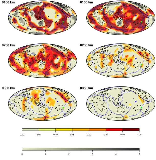
Fig. 1: Shear velocity and attenuation in the upper mantle. Panels a-c-e-g:
280
perturbations in shear wave velocities from DR2020s shown in percent with respect to a 281
mean value Vref given in km s-1 above the colour scale. Panels b-d-f-h: maps of our Qs
282 tomographic model QsADR17 at different depths in the upper mantle. Qs is plotted with a 283 logarithmic scale. Its geometric average is given above the colour scale. Hotspot locations 284 are shown with black triangles. 285 286 287 288 Fig. 2: Scatter plot depicting the observed shear attenuation as a function of shear 289
velocity compared with theoretical predictions. The velocities (from DR2020s) and
290 attenuation values (from QsADR17) are plotted at 100 km (panel a), 150 km (panel b) and 291 200 km depth (panel c). Each dot corresponds to a geographical location. The dark blue 292 and light blue curves are the theoretical predictions assuming a pyrolitic composition34 in 293
the absence of melt using the anelasticity models of Takei4 and Jackson et al.13,
294 respectively. The upper colour scale indicates the amount of melt in percent required to 295 explain our observations using Takei4’s model. Adding melt enables to lower the predicted 296 velocity without changing Qs. The lower grey scale indicates the misfit in percent between 297
theory and observations, in regions where Vs is too high and cannot be reconciled with 298
model predictions assuming a pyrolitic mantle. 299
300 301
Fig. 3: Melt content at different depths in the upper mantle. This melt content is
302
derived from the joint interpretation of QsADR17 and DR2020s. The colour coding is 303
identical to Figure 2. Melt content in percent is indicated with warm colour from ivory 304
(0% melt) to brown (0.4 to 0.7% melt). The grey scale indicates the misfit in percent 305
between theory and observations, in regions where Vs is too high compared with 306 predictions. Hotspots locations are indicated with black triangles. The blue and green stars 307 indicate the location of the NoMELT and MELT experiments, respectively. 308 309 310 311
Fig. 4: Percentage of melt at different depths as a function of absolute plate velocity.
312
(The velocities29 are expressed in a no-net-rotation reference frame. The percentage of
313
melt is averaged for all geographical points with similar plate velocities, using a sliding 314
window of ±2 cm yr-1. The amount of melt increases significantly in the asthenosphere
315
(100-200 km) for plate velocities between 3 and 5 cm yr-1. This result links with previous
316
observations that only plates moving faster than 4 cm yr-1 can organize the flow at large
317
scale in the underlying asthenosphere8, suggesting that melt reduces viscosity9 and
318
facilitates large-scale crystal alignment. 319
Methods 321
Qs and Vs tomographic models. Figure 1 presents maps of DR2020s, a new 322 global Vs model and QsADR17 a recent global Qs model30. Both models are built 323 from the same massive Rayleigh wave measurements31, and are obtained from a 324 similar tomographic procedure. The first step is an automated waveform inversion 325
approach which was applied to approximately 375,000 Rayleigh seismograms31. 326
From a single surface wave seismogram, the waveform inversion extracts 327
simultaneously a path-average depth-dependent shear velocity profile, Vs, and 328
quality factor, Qs. By jointly interpreting the amplitude and phase of each 329
waveform, we ensure that the interplay between Vs and Qs is accounted for, and 330
that the shear quality factor and velocity profiles are constrained within the same 331
period range. The waveform analysis is performed in the period range 50-250 s 332
and accounts for the fundamental and up to the 5th higher mode of Rayleigh 333
waves, thus ensuring a good depth resolution for Vs and Qs from 50 km depth 334
down to the transition zone. It is a non-linear iterative process, which also 335 produces frequency-dependent phase velocity and attenuation curves compatible 336 with the recorded waveform. The effect of physical dispersion due to attenuation is 337 accounted for in the modelling. 338
The second step is a regionalization of the 1D path-average models. DR2020s is 339
obtained from the regionalization at each depth of the path-average Vs models 340
using a continuous regionalization approach31. This tomographic inversion yields 341
3D absolute velocities. QADR17, a global model of Rayleigh-wave attenuation was 342
obtained after adapting the same regionalization approach to our dataset of 343
Rayleigh wave attenuation curves, parameterized as ln(Q)32. The regionalisation of 344
the path-average attenuation curves accounts for frequency-dependent effects like 345
focussing-defocussing, which can have important effects on the amplitude of 346
Rayleigh waves. The logarithmic parameterization brings the distribution of the 347
quality factor dataset close to a Gaussian, allows the large variations of Q 348 documented by local seismic studies and guarantees to avoid negative attenuation 349 values in the inverted model. The horizontal smoothing in DR2020s and QADR17 350 is determined by a Gaussian a priori covariance function controlled by an angular 351 correlation length. Adenis et al.32 chose a conservative value of 10° (meaning that 352
the Q model is resolved accurately up to spherical harmonic 12). Debayle and 353 Ricard31 used a shorter correlation length of 3.6° for their Vs model DR2012. We 354 re-inverted their dataset using a correlation length of 10° in order to obtain a Sv-355 wave tomographic model at the same horizontal resolution and vertical smoothing 356
than QsADR17. To minimize biases due to un-modelled radial anisotropy, we 357
computed the isotropic Voigt average of our Sv model and the Sh model obtained 358
by adding the radial anisotropy of PREM to our Sv model. The resulting isotropic 359
model DR2020s is plotted in Figure 1. Using other 1D or 3D models of radial 360
anisotropy does not affect our conclusions, as discussed below. QsADR17 was 361
obtained from the inversion at depth of QADR1730, using the same vertical 362
smoothing as for DR2020s. DR2020s and QsADR17 are therefore consistent since 363
they are derived from the simultaneous inversion of the same waveforms and 364 inverted using the same regionalization approach with the same Gaussian filtering. 365 Prediction of Qs and Vs using a temperature-dependent model4. The dark blue 366 curve in Figure 2 is obtained by predicting Vs and Qs at each depth for a range of 367 temperatures, using a temperature-dependent anelasticity model4 and assuming a 368 pyrolitic composition16. This model parameterizes the relaxation spectrum with a 369
small number of variables determined from experimental data. It accounts for a 370
monotonic background spectrum plus a broad temperature-dependent absorption 371
peak in the seismic frequency band, whose amplitude and width increase below 372
the solidus. This produces a significant enhancement of polycrystal anelasticity 373
before melting. This pre-melting effect induces large Vs reductions under the 374
solidus. We choose the solidus according to Hirschman33. We use the model 375
parameters given in Tables 1 and 2 of Takei4, except for the unrelaxed shear 376
modulus 𝜇!. We estimate 𝜇! for a pyrolitic mantle using the mineralogic phase 377
diagram computed by the Perple X software34. In Figures S15-S16 we show the 378 results obtained with the shear modulus of Takei4, which reduces the amount of 379 melt in oceanic regions but fails to explain our ln(Qs)-Vs observations beneath old 380 oceanic basins at 100 km depth. It also significantly increases the misfit beneath 381 continents. 382 Prediction of Qs and Vs from the experimental results of Jackson et al.13. The 383
light blue curve in Figure 2 is obtained by a two-step process. First, we use 384
experimental results on melt-free polycrystalline olivine to predict a theoretical 385
quality factor Qt. Computations are performed in the temperature range 800-1800
386
K and the pressure range 1.49-12.99 GPa, corresponding to the depth range 50-387 390 km. We use the following relation13 : 388 𝑄!!! 𝑇!, 𝑇, 𝑃, 𝑑 = 𝐴 𝑇!𝑑!!exp −(𝐸 + 𝑃𝑉) 𝑅𝑇 ! Eq. A.1 389 In this formulation, 𝑄!!!at period T 0 depends on the temperature T, the pressure P 390
and to a lesser extent the grain size d. R is the gas constant, E is the activation 391
energy and V is the activation volume. Table S1 summarizes the values of the 392
different parameters of Eq. A.1. In the range of values compatible with 393
experiments13, we choose T0=100 s, the average period of our long period Rayleigh 394
waves and d=0.01m. The theoretical curves corresponding to Eq. A1 are shown in 395
Figure S9, with the effect of changing grain size. 396
Second, we use Perple X34 to estimate an isotropic Vs for a pyrolitic model16. We 397
compute Vs for the same temperatures and pressures as Qt. Perple_X produces
unrelaxed S-wave velocities at infinite frequency, above the absorption band of 399 seismic attenuation, while our long period (>50 s) seismic surface waves are likely 400 to see relaxed velocities. We therefore correct for the effect of anelasticity on Vs35 : 401 𝑉!!= 𝑉 !! 1 −!! !!(! !,!,!,!) !!"# !" ! Eq. A.2 402
where 𝑉!!is the unrelaxed velocity and 𝑉!! is the velocity corrected from the effect
403
of attenuation. According to Eq. A2, the stronger the attenuation, the stronger the 404
velocity reduction is. The light blue curve in Figure 2 is finally obtained by plotting 405
at a given depth the obtained ln(𝑄!) as a function of 𝑉!! for each temperature.
406 Comparison between our observations and the theoretical relations. At each 407 geographical location and depth, we extract the observed value of Qs in QsADR17 408 and Vs in DR2020s and we compare our observations with the chosen theoretical 409
relation. We consider that a theoretical curve is compatible with a given Vs-Qs 410
observation if it falls within ±1% and ±10% of the Vs and ln(Qs) observations, 411
respectively (Figure 2). These errors are on the conservative side of recent 412
estimates36,37. If the theoretical relation cannot explain our observations, two 413 situations can arise: 1) the observed Vs is lower than the theoretical V!!. In this case 414 melt can be added to reduce V!!. This is done assuming melt has no effect on Qs; 2) 415 the observed Vs is higher than V!!. This is mostly the case under continents and can 416
be explained by the depletion of the pyrolitic mantle increasing the theoretical 417 V!!18. 418 Effect of grain size. Grain sizes in the shallow upper mantle are likely 1-20 mm as 419 observed in upper mantle xenoliths, harzburgite and dunite bodies13. The effect of 420 grain size on Eq. A1 is shown in Figure S9. The blue areas around the theoretical 421 curves cover the influence of grain size from 1 mm (bottom dot curve) to an upper 422
bound of 100 mm (upper dashed curve). For a given value of Qs, increasing the 423
grain size increases the temperature and therefore decreases the velocity. As melt 424
is required for explaining slow velocities, increasing grain size will decrease the 425
amount of melt required to explain our observations. Using the equation A1 426
proposed by Jackson, we show in Figure S12 melt distributions obtained for 427
d=0.01 m and in Figure S17 those for the extreme value d=0.1 m, which minimizes
428
the amount of melt required in the LVZ. Maps in Figure S17 are similar to those of 429
Figure S12 with a smaller amount of melt. However, in both cases, amounts of 430 melt are larger than for our preferred model using the equations of Takei4 (Figure 431 3). 432 Amounts of melt. Although the amount of melt present in the LVZ depends on the 433 choice of the anelasticity model and on the effect of melt on Vs, we show in Figures 434
S12, S16, S17, S18 that different choices of parameters yields similar maps and 435
that melt fractions away from source regions always stay below 1%, in agreement 436
with the partially molten asthenosphere model2. We note however that our 437
preferred anelasticity model4 generally explains our Vs and ln(Qs) observations 438
without the need of partial melt above and below the asthenosphere (Figure 3). 439
This is therefore a conservative choice, able to reconcile our Vs and ln(Qs) 440
observations in most of the upper mantle, while minimizing the amount of melt 441
required in the LVZ. 442
Effect of radial anisotropy. We used the anisotropic parameter ξ=(Vsh/Vsv)2 of 443
PREM to convert our Sv observations into an isotropic model, DR2020s. We 444
checked that 3D models of ξ obtained from anisotropic models like SEMUM238 or 445
S362ANI39 would not affect our main conclusions. As an example, Figure S1 is 446
similar to Figure 3 but based on our Sv observations corrected with the 447
anisotropic ξ parameters of SEMUM2 (Figure S2). Only minor changes are 448
observed (for example in the Pacific or Indian oceans at 150 and 200 km), but 449
none that would change the interpretations of this paper. The lateral variations of ξ 450 in SEMUM2 (Figure S2) are too small to affect our results. To confirm this point, 451 we computed the anisotropy ξ that would be needed to account for the discrepancy 452
between observed Qs and Vs, without invoking mantle depletion or partial melt 453
(Figure S3). Comparison of this figure with Figure S2 shows that neither the 454
patterns nor the amplitude would fit (a 3 to 4 times larger anisotropy than in 455
SEMUM2 would be needed to explain our observations). The anisotropy therefore 456
does not affect our conclusions. 457
Elastically accommodated grain boundary sliding (EAGBS) hypothesis. 458
Anelastic relaxation caused by EAGBS can produce a sharp velocity reduction and 459
may explain the LAB and the mid-lithosphere discontinuity observed beneath 460
continents40. We tested the EAGBS hypothesis as an alternative explanation to 461
partial melting for reconciling Vs and Qs in the LVZ. EAGBS is characterized by a 462
sharp attenuation peak at a characteristic frequency 𝜔!"#$%, followed by a diffused 463
absorption band at lower frequencies. We first compute the characteristic 464
frequency for the transition between unrelaxed and relaxed shear moduli. It is 465 given by Karato et al.,40 : 466 𝜔!"#$%= 𝐴. 𝑑!!. 𝑒𝑥𝑝 −!∗!!!∗ !.! . 1 + !! !!! ! Eq. A3 467
where Cw is the water content in wt%, A=2.3x10⁻¹⁴ m s-1, Cw0=10-4 wt%, r=1,
468
E*=350 kJ mol-1, V*=10-6 m3, d=5x10⁻³ m. Following Cobden et al.7 we assume a dry 469
mantle with Cw=10-6 wt %. 470
Surface waves analysed at frequencies lower than 𝜔!"#$% should see relaxed 471
velocities within the absorption band (see Fig. SI-2 of Karato et al.40), providing 472
depth and temperature are within the activation ranges of EAGBS. EAGBS is 473
activated between 60 and 160 km depth in the temperature range 900-1,350 K. We 474
consider that EAGBS may affect the interpretations of our long period (>40 s) Qs 475
and Vs maps when 𝜔!"#$%> 0.025 Hz and, from figure 4 of Karato et al.40, in the 476 following temperature ranges for the depths of our tomographic inversion: 477 • 70 km: 930-1,140 K 478 • 90 km: 980-1,180 K 479 • 100 km: 1,010-1,220 K 480 • 125 km: 1,060-1,270 K 481 • 150 km: 1,130-1,330 K 482
Regions where EAGBS can apply are displayed in green in Figure S4. These 483 regions correspond mostly to continental areas. Assuming that EAGBS correction 484 applies, Karato et al.40 list three alternative formulations for the velocity reduction. 485 The Ghahremani41 equation, which produces the smallest velocity reduction is : 486 𝑉!!"#$% = 𝑉!!. !.!"!!.!"! !!! ∙ !!! !.!"!!.!"! Eq. A.4 487
where 𝜈 is the Poisson's ratio (~0.3 for upper mantle minerals). Regions where 488
this can reconcile our Vs and Qs observations are displayed in red in Figure S4. 489
The two other formulations give too large velocity reduction. Figure S4 shows that 490
EAGBS fails at reconciling our long period observations, excepted in a few localized 491
regions (in red). This does not preclude EAGBS to play a significant role in 492
explaining the sharp velocity reduction associated with the LAB, which cannot be 493
resolved by long period surface waves. However, the strong velocity reduction 494
observed within the LVZ requires another mechanism. 495
Effect of composition. Compositional heterogeneities exist in the upper mantle, 496
likely in the domain limited by pyrolite, harzburgite and pyroxenite42. Here, we 497
check the effect of changing the composition from pyrolite to these end-members 498
using Perple X34 to compute the velocities. Pyroxenites have variable bulk 499
compositions43 and we consider both a silica-deficient composition (see, Stixrude 500 and Lithgow-Bertelloni44, Table 1) and a silica-excess composition similar to that 501 of a subducted basalt (see, Xu et al.,16, Table 1). A silica-excess pyroxenite would 502
only be faster that pyrolite after eclogitization, below 150 km depth (Figure S5, 503
orange curve). At 100 km depth, a mantle made entirely of silica-excess pyroxenite 504
would be too slow to explain the observed velocities (Figure S6). At larger depth, 505
after eclogitization, it would lead to large melt fractions (Figure S6). The silica-506
deficient pyroxenite and the harzburgite are characterized at asthenospheric 507 conditions by much faster or comparable velocities than pyrolite (Figure S5) and 508 hence cannot explain the low velocities that we attribute to the presence of melt. 509 Harzburgite would give melt fractions and distribution similar to pyrolite (Figure 510 S7), while the silicate-deficient pyroxenite would lead to higher melt fractions (up 511
to 1.7%) and a ubiquitous melt presence below 150 km depth (Figure S8). 512
Pyroxenite, whether enriched or depleted in silica, should only be present in a 513
small proportion (~5%)42 that hardly affects the seismic velocities of the 514 peridotitic mantle. At any rate, large-scale chemical heterogeneities (> 1000 km) 515 are not likely to exist in the LVZ, where viscosity is small (below 1020 Pa s) and the 516 convective mantle should be well stirred and mixed. Therefore, our observations 517 cannot be explained by reasonable variations of compositions in the LVZ. 518
Possible effect of water. Although, it has been recently shown that in olivine, 519
wave-speed and attenuation are insensitive to water10, some previous studies had 520
suggested an effect of water quantified following the equation45: 521 𝑄!!! 𝑇 !, 𝑇, 𝑃, 𝐶!", 𝑑 = 𝐴 𝑇!𝑑!! !!!" !"(!"#) ! exp −(𝐸 + 𝑃𝑉) 𝑅𝑇 ! Eq. A.5 522 where COH is the water concentration, r is a dimensionless constant and all other 523 parameters are as in Eq. A1. The average H2O content of Earth’s upper mantle is 524
estimated in the range 50-200 ppm46. We test a value close to the upper bound 525
(COH=1000H/106 Si, corresponding to 125 ±75 ppm by weight of water) with r=1, a
526
standard value for moderate water content and COH(ref)=50H/106 SI7. The
527
corresponding theoretical curves are shown in blue on Figure S9. At fixed 528
temperature, water increases attenuation. However to keep Q constant, an 529
increase of water content must be balanced by a decrease of temperature and 530
therefore by a higher expected velocity 𝑉!!. Reconciling this higher 𝑉
!! with our
531
observations requires larger amounts of melt (Figure S10). Therefore, if there were 532
an effect of water on Vs and Qs, it would increase the required amount of melt. 533 Effect of melt on attenuation. A small amount of melt might have a large effect on 534 attenuation47 in the case of grain boundary sliding, where a broad dissipation peak 535 is observed in the seismic frequency band. Body wave studies have reported low 536
Qs values at short period (1s) with Qs≤25 beneath the Juan de Fuca and Gorda 537
ridges48 and 25≤Qs≤80 in the back-arc mantle of Central America, the Marianas 538
and the Lau Basin49. A recent experimental study suggests that 0.2% of melt 539
produces Qs=483. However such a large effect of melt on Qs is difficult to reconcile 540
with long period (>30 s) surface waves observations of Qs=80 beneath the fast 541
spreading southern East pacific Rise20 where up to 1-2% of melt is expected50. If 542
the attenuation mechanism is melt squirt, then the dissipation peak may lie outside 543
the seismic frequency band and cause little attenuation. Model calculations51 , long-544
period surface waves20 and experiments12 favour such interpretation. This is also 545
supported by our long period (100 s) global surface wave tomographic models, 546 which suggest that strong Vs and Qs reductions are not necessarily correlated30,32. 547 For these reasons, we assume that in the period range of surface waves (50-250s), 548 melt does not significantly affects attenuation and we neglect its effect on Qs. 549
Temperature in the upper mantle. Our Qs and Vs seismic models are interpreted 550
using mineral physics results4,13. These experimental results are valid at temperatures 551
larger than 900°C or 1000°C, which are reached at the base of the lithosphere and in the 552
asthenosphere. The predictions of our model can be checked with respect to the well-553
known thermal behaviour of the cooling oceanic lithosphere52,53 although this is 554
certainly pushing the model outside its applicability range. Figure S19 (panel a), 555
displays the temperature variations beneath the Pacific as a function of sea-floor age 556
predicted from our seismic models using experimental results4. It demonstrates that 557
even at depths shallower than 100 km, we retrieve the well-known age-dependence of 558
temperature in oceanic regions (we also pick up the cold signal of the West Pacific 559
subductions at old ages). However, our temperature variations between the ridge and an 560
old lithosphere (~100°) are lower than the predictions of the plate-cooling model (250° 561
at 75 km depth, panel b). Panel c displays the quality factors that would be deduced 562
from the plate-cooling model using the experimental results4 used in this paper. In the 563
oceanic lithosphere, Qs values much greater than 2000 (ln(Qs) > 7.6) would be 564
predicted, that cannot be retrieved by long period seismology. The limitations of 565
experimental data at low temperatures together with the inability of surface wave 566
seismology to quantify precisely negligible attenuations, explain why we do not 567
interpret results at depths shallower than 100 km. Below the oceanic plates, Figure S14, 568
panel g shows that our predicted temperatures beneath oceans are perfectly compatible 569
with geodynamic and petrologic expectations. In agreement with our findings, under 570 oceans, the average 1D temperature profile is above the solidus4 and the adiabat54 571 in the depth range 100-200 km, where we predict partial melting. This overshoot 572 of the temperature, above the adiabat, is indeed found in all numerical simulations 573 of mantle convection55. Under continents, the temperature appears to be below the 574
solidus4 and the adiabat54. It reaches the adiabat around 250 km depth (Figure 575
S14, panel g). 576
Compatibility of our results with electrical conductivity. Our results are 577
consistent with the interpretation of a number of recent studies of electrical 578
conductivity. In the depth range 100-150 km, the joint interpretation of electrical 579 and seismic data56 requires 0.3-2.5% of melt beneath the mid-Atlantic ridge, 1% or 580 less melt beneath Hawaï and less than 5% of melt beneath the East-pacific rise, in 581 good agreement with Figure 3. We also confirm the absence of melt in the region 582 of the NoMELT experiment19, in agreement with conductivity data in this region25. 583
Previous experimental results suggest that between 0.3 and 2% of hydrous 584
basaltic melt can account for the observed electrical conductivity in the LVZ27. A 585
more recent study57 has refined these results by simultaneously measuring wave 586
velocity and electrical conductivity on a simplified partial melt analogue. They 587 conclude that the low velocity zone away from spreading ridges can be explained 588 by 0.3-0.8% volatile-bearing melt, the upper bound of our observations. 589 Implications for viscosity. The variation of viscosity as a function of melt content 590
occurs in two steps9. The onset of melting brings already a significant effect on 591 viscosity when a connected network of melt tubules is formed. The viscosity η is 592 expected to decrease by one or two orders of magnitude before the melt fraction φ 593 reaches 0.1%. For larger melt content, η decreases further9 with dln(η)/dφ = -26 594
but this effect is minor for the low melt content that we observe. Under oceanic 595 plates where φ is around 0.3%, η should be one or two orders of magnitude lower 596 than under continents. 597 Data availability: The dataset generated during this study (3D Vs, Qs models and 598
melt fraction models) is available as IRIS data products at 599
https://doi.org/10.17611/dp/emc.2020.dbrdnature.1. 600
Code availability: Numerical modelling codes related with this paper can be 601
downloaded from https://doi.org/10.17611/dp/emc.2020.dbrdnature.1. Requests 602
about the numerical modelling codes associated with this paper should be sent to 603
[email protected]. Most figures were created with open software GMT 604 4.5.13. 605 Competing interest: The authors declare no competing interests. 606 References from Methods: 607 608 30. Adenis, A., Debayle, E. & Ricard, Y. Attenuation tomography of the upper mantle. Geophys. 609 Res. Lett. 44, (2017). 610 31. Debayle, E. & Ricard, Y. A global shear velocity model of the upper mantle from fundamental 611 and higher Rayleigh mode measurements. J. Geophys. Res., Sol. Earth., 117, (2012). 612 32. Adenis, A., Debayle, E. & Ricard, Y. Seismic evidence for broad attenuation anomalies in the 613 asthenosphere beneath the Pacific Ocean. Geophys. J. Int. 209, 1677–1698 (2017). 614 33. Hirschmann M. M. Mantle solidus: Experimental constraints and the effects of peridotite 615 composition. Geochemistry Geophys. Geosystems 1, 1042 (2000). 616 34. Connolly, J. A. D. Computation of phase equilibria by linear programming: A tool for 617 geodynamic modeling and its application to subduction zone decarbonation. Earth Planet. 618 Sci. Lett. 236, 524–541 (2005). 619 35. Karato, S. Importance of anelasticity in the interpretation of seismic tomography. Geophys. 620 Res. Lett. 20, 1623–1626 (1993). 621 36. Zaroli, C. Global seismic tomography using Backus-Gilbert inversion. Geophys. J. Int. 207, 622 876–888 (2016). 623 37. Resovsky, J., Trampert, J. & der Hilst, R. D. Error bars for the global seismic Q profile. Earth 624 Planet. Sci. Lett. 230, 413–423 (2005). 625 38. French, S., Lekic, V. & Romanowicz, B. Waveform Tomography Reveals Channeled Flow at 626 the Base of the Oceanic Asthenosphere. Science 342, 227–230 (2013). 627 39. Kustowski, B., Ekstrom, G. & Dziewonski, A. M. Anisotropic shear-wave velocity structure of 628 the Earth’s mantle: A global model. J. Geophys. Res. 113, (2008). 629 40. Karato, S. I., Olugboji, T. & Park, J. Mechanisms and geologic significance of the mid-630 lithosphere discontinuity in the continents. Nat. Geosci. 8, 509–514 (2015). 631 41. Ghahremani, F. Effect of grain boundary sliding on anelasticity of polycrystals. Int. J. Solids 632 Struct. 16, 825–845 (1980). 633 42. Hirschmann, M. M. & Stolper, E. M. A possible role for garnet pyroxenite in the origin of the 634 ‘“garnet signature”’ in MORB. Contrib. Miner. Pet. 124, 185–208 (1996). 635 43. Lambart, S., Laporte, D. & Schiano, P. Markers of the pyroxenite contribution in the major-636 element compositions of oceanic basalts: Review of the experimental constraints. Lithos 637 160, 14–36 (2013). 638 44. Stixrude, L. & Lithgow-Bertelloni, C. Mineralogy and elasticity of the oceanic upper mantle: 639 Origin of the low-velocity zone. J. Geophys. Res. Solid Earth 110, B03204 (2005). 640 45. Behn, M. D., Hirth, G. & Elsenbeck, J. R. Implications of grain size evolution on the seismic 641 structure of the oceanic upper mantle. Earth Planet. Sci. Lett. 282, 178–189 (2009). 642 46. Hirschmann, M. M. Water, melting, and the deep Earth H2O cycle. Annu. Rev. Earth Planet. 643 Sci. 34, 629–653 (2006). 644 47. Faul, U. H., Fitz Gerald, J. D. & Jackson, I. Shear wave attenuation and dispersion in melt-645 bearing olivine polycrystals: 2. Microstructural interpretation and seismological 646 implications. J. Geophys. Res. Solid Earth 109, 1–20 (2004). 647 48. Eilon, Z. C. & Abers, G. A. High seismic attenuation at a mid-ocean ridge reveals the 648 distribution of deep melt. Sci. Adv. 3, (2017). 649 49. Abers, G. A. et al. Reconciling mantle attenuation-temperature relationships from 650 seismology, petrology, and laboratory measurements. Geochem., Geophy., Geosy., 15, 3521– 651 3542 (2014). 652
50. Dunn, R. A. & Forsyth, D. W. Imaging the transition between the region of mantle melt 653 generation and the crustal magma chamber beneath the southern East Pacific Rise with 654 short-period Love waves. J. Geophys. Res. Solid Earth 108, 2352 (2003). 655 51. Hammond, W. C. & Humphreys, E. D. Upper mantle seismic wave attenuation: Effects of 656 realistic partial melt distribution. J. Geophys. Res. Solid Earth 105, 10987–10999 (2000). 657 52. Turcotte, D. L. & Schubert, G. Geodynamics: Applications of Continuum Physics to Geological 658 Problems. (John Wiley & Sons, New York, 1982). 659 53. Stein, C. A. & Stein, S. A model for the global variation in oceanic depth and heat flow with 660 lithospheric age. Nature, 359, 123–129 (1992). 661 54. Katsura, T. et al. Adiabatic temperature profile in the mantle. Phys. Earth Planet. Inter. 183, 662 212–218 (2010). 663 55. Curbelo, J. et al. Numerical solutions of compressible convection with an infinite Prandtl 664 number: comparison of the anelastic and anelastic liquid models with the exact equations. J. 665 Fluid Mech. 873, 646–687 (2019). 666 56. Pommier, A. & Garnero, E. J. Petrology-based modeling of mantle melt electrical conductivity 667 and joint interpretation of electromagnetic and seismic results. J. Geophys. Res., Sol. Earth., 668 119, 4001–4016 (2014). 669 57. Freitas, D., Manthilake, G., Chantel, J., Bouhifd, M. A. & Andrault, D. Simultaneous 670 measurements of electrical conductivity and seismicwave velocity of partially molten 671 geological materials: effect of evolving melt texture. Phys. Chem. Miner. 46, 535–551 (2019). 672 673
−10 −5 −2 2 5 10 Vsref=4.41 50 100 200 500 1000 Qref=194 −10 −5 −2 2 5 10
150 km
Vsref=4.41 50 100 200 500 1000150 km
Qref=192 −10 −5 −2 2 5 10200 km
Vsref=4.44 50 100 200 500 1000200 km
Qref=203 −10 −5 −2 2 5 10300 km
Vsref=4.60 50 100 200 500 1000300 km
Qref=213a
b
c
d
e
f
g
h
2.0 2.5 3.0 3.5 4.0 4.5 5.0 ln(Qs) 4.0 4.2 4.4 4.6 4.8 2.0 2.5 3.0 3.5 4.0 4.5 5.0 ln(Qs) 4.0 4.2 4.4 4.6 4.8 2.0 2.5 3.0 3.5 4.0 4.5 5.0 ln(Qs) 4.0 4.2 4.4 4.6 4.8 0100 km 2.0 2.5 3.0 3.5 4.0 4.5 5.0 5.5 6.0 6.5 7.0 7.5 8.0 ln(Qs) 4.0 4.2 4.4 4.6 4.8 2.0 2.5 3.0 3.5 4.0 4.5 5.0 5.5 6.0 6.5 7.0 7.5 8.0 ln(Qs) 4.0 4.2 4.4 4.6 4.8 2.0 2.5 3.0 3.5 4.0 4.5 5.0 5.5 6.0 6.5 7.0 7.5 8.0 ln(Qs) 4.0 4.2 4.4 4.6 4.8 b 0150 km 2.0 2.5 3.0 3.5 4.0 4.5 5.0 5.5 6.0 6.5 7.0 7.5 8.0 ln(Qs) 4.0 4.2 4.4 4.6 4.8 Vs (km/s) 2.0 2.5 3.0 3.5 4.0 4.5 5.0 5.5 6.0 6.5 7.0 7.5 8.0 ln(Qs) 4.0 4.2 4.4 4.6 4.8 Vs (km/s) 2.0 2.5 3.0 3.5 4.0 4.5 5.0 5.5 6.0 6.5 7.0 7.5 8.0 ln(Qs) 4.0 4.2 4.4 4.6 4.8 Vs (km/s) c 0200 km 0.00 0.01 0.10 0.15 0.20 0.30 0.40 1.00 0 1 2 3 4 5
0200 km 0250 km 0300 km 0350 km 0.00 0.01 0.10 0.15 0.20 0.30 0.40 0.70 5 4 3 2 1 0
a
b
c
d
e
f
0
1
2
3
4
5
6
7
8
Plate velocity (cm/year)
0
0.1
0.2
Percentage of melt (%)
250 km
350 km
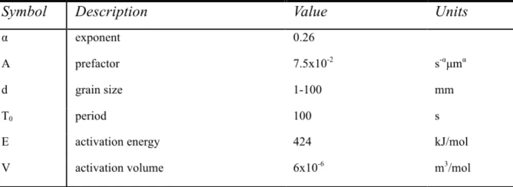
α exponent 0.26
A prefactor 7.5x10⁻² s-αµmα
d grain size 1-100 mm
T0 period 100 s
E activation energy 424 kJ/mol
V activation volume 6x10⁻⁶ m3/mol
Table S1: Reference parameters for Eq.A.1 after Jackson et al.1
Fig. S1: same as Figure 2 but the color scales indicate the departure from the model of Jackson et al.1 (light blue curve), for a grain size of 10 mm. The upper color scale indicates the amount of melt in percent required to explain our observations (ivory color from 0 to 0.01% of melt underlines data for which the model can reconcile our Qs and Vs observations). The lower grey scale indicates the misfit in percent between theory and observations, in regions where Vs is too high and cannot be reconciled with model predictions. 2.0 2.5 3.0 3.5 4.0 4.5 5.0 ln(Qs) 4.0 4.2 4.4 4.6 4.8 2.0 2.5 3.0 3.5 4.0 4.5 5.0 ln(Qs) 4.0 4.2 4.4 4.6 4.8 2.0 2.5 3.0 3.5 4.0 4.5 5.0 ln(Qs) 4.0 4.2 4.4 4.6 4.8 0100 km 2.0 2.5 3.0 3.5 4.0 4.5 5.0 5.5 6.0 6.5 7.0 7.5 8.0 ln(Qs) 4.0 4.2 4.4 4.6 4.8 2.0 2.5 3.0 3.5 4.0 4.5 5.0 5.5 6.0 6.5 7.0 7.5 8.0 ln(Qs) 4.0 4.2 4.4 4.6 4.8 2.0 2.5 3.0 3.5 4.0 4.5 5.0 5.5 6.0 6.5 7.0 7.5 8.0 ln(Qs) 4.0 4.2 4.4 4.6 4.8 0150 km 2.0 2.5 3.0 3.5 4.0 4.5 5.0 5.5 6.0 6.5 7.0 7.5 8.0 ln(Qs) 4.0 4.2 4.4 4.6 4.8 Vs (km/s) 2.0 2.5 3.0 3.5 4.0 4.5 5.0 5.5 6.0 6.5 7.0 7.5 8.0 ln(Qs) 4.0 4.2 4.4 4.6 4.8 Vs (km/s) 2.0 2.5 3.0 3.5 4.0 4.5 5.0 5.5 6.0 6.5 7.0 7.5 8.0 ln(Qs) 4.0 4.2 4.4 4.6 4.8 Vs (km/s) 0200 km 0.00 0.01 0.10 0.15 0.20 0.30 0.40 1.00 0 1 2 3 4 5
Fig. S2: same as Figure 3 but color scales indicate the departure from the model of Jackson et al.1, for a grain size of 10 mm. Melt content in percent is indicated with warm colors (upper color scale) from ivory (0% melt) to brown (0.4 to 0.7% melt). The lower grey scale indicates the misfit in percent between the theory and observations, in regions where Vs is too high compared with predictions. 0100 km 0150 km 0200 km 0250 km 0300 km 0350 km 0.00 0.01 0.10 0.15 0.20 0.30 0.40 1.00 0 1 2 3 4 5
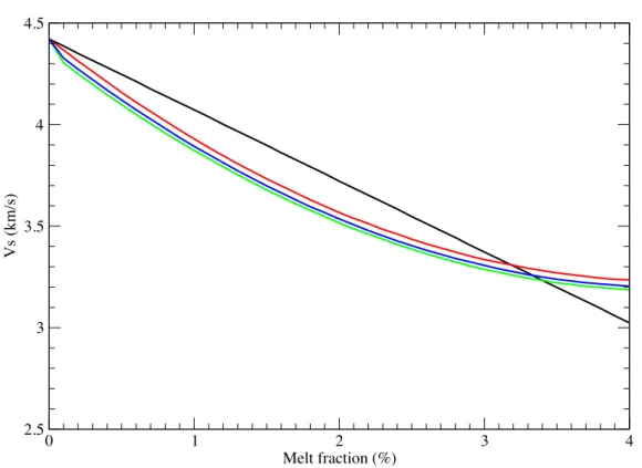
Fig. S3: Dependence of shear velocity on melt fraction 𝜑. The linear Vs reduction of 7.9% per percent of melt2 is shown in black from a reference velocity Vref. The polynomial expression ( 𝑉! = 0.065𝜑!− 0.5565𝜑 + 𝑉
!"#) derived from experimental results3 is
shown in red. The anelastic effect expected for seismic waves at high temperature4 is shown assuming Qs=80, the value of PREM5 in the asthenosphere, for two values of α (blue curve for α=0.38 and green curve for α=0.26). For small melt fractions (<1%), a stronger Vs reduction is obtained using the polynomial expression and the choice of α has a small effect. 0 1 2 3 4 Melt fraction (%) 2.5 3 3.5 4 4.5 Vs (km/s)
Fig. S4: same as Fig. 3 but using a linear 7.9% Vs reduction per percent of melt2 instead of the polynomial expression derived from experimental results3. The upper color scale is slightly modified to allow melt content up to 1% (the maximum value at 100 km depth). 0200 km 0250 km 0300 km 0350 km 0.00 0.01 0.10 0.15 0.20 0.30 0.40 1.00 0 1 2 3 4 5
Fig. S5: same as Figure 2 but the unrelaxed shear modulus 𝜇! needed to compute the temperature-dependent model (dark blue curve) is calculated using parameters proposed for of the temperature model of the Pacific6, instead of those deduced from Perple X assuming a pyrolitic composition. 2.0 2.5 3.0 3.5 4.0 4.5 5.0 ln(Qs) 4.0 4.2 4.4 4.6 4.8 2.0 2.5 3.0 3.5 4.0 4.5 5.0 ln(Qs) 4.0 4.2 4.4 4.6 4.8 2.0 2.5 3.0 3.5 4.0 4.5 5.0 ln(Qs) 4.0 4.2 4.4 4.6 4.8 0100 km 2.0 2.5 3.0 3.5 4.0 4.5 5.0 5.5 6.0 6.5 7.0 7.5 8.0 ln(Qs) 4.0 4.2 4.4 4.6 4.8 2.0 2.5 3.0 3.5 4.0 4.5 5.0 5.5 6.0 6.5 7.0 7.5 8.0 ln(Qs) 4.0 4.2 4.4 4.6 4.8 2.0 2.5 3.0 3.5 4.0 4.5 5.0 5.5 6.0 6.5 7.0 7.5 8.0 ln(Qs) 4.0 4.2 4.4 4.6 4.8 0150 km 2.0 2.5 3.0 3.5 4.0 4.5 5.0 5.5 6.0 6.5 7.0 7.5 8.0 ln(Qs) 4.0 4.2 4.4 4.6 4.8 Vs (km/s) 2.0 2.5 3.0 3.5 4.0 4.5 5.0 5.5 6.0 6.5 7.0 7.5 8.0 ln(Qs) 4.0 4.2 4.4 4.6 4.8 Vs (km/s) 2.0 2.5 3.0 3.5 4.0 4.5 5.0 5.5 6.0 6.5 7.0 7.5 8.0 ln(Qs) 4.0 4.2 4.4 4.6 4.8 Vs (km/s) 0200 km 0.00 0.01 0.10 0.15 0.20 0.30 0.40 0.70 0 1 2 3 4 5
Fig. S6: same as Figure 3 but instead to estimate the unrelaxed shear modulus 𝜇! using Perple X and a pyrolitic model, we use fitting parameters of the temperature model for the Pacific6. 0200 km 0250 km 0300 km 0350 km 0.00 0.01 0.10 0.15 0.20 0.30 0.40 0.70 0 1 2 3 4 5
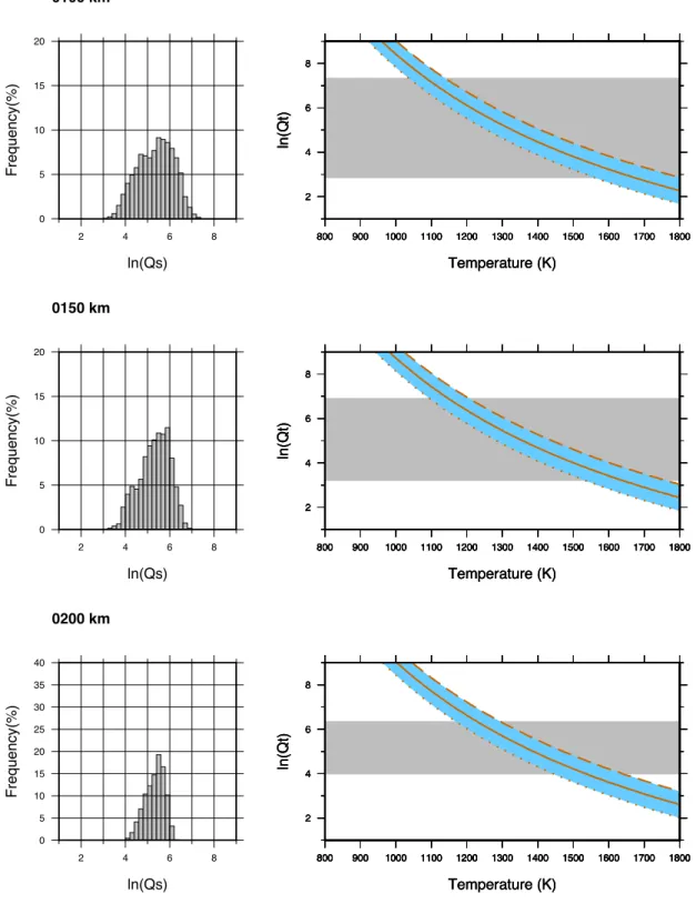
Fig. S7: Left column: Histograms of the distribution of ln(𝑄!) values extracted at 100 (top), 150 (middle) and 200 (bottom) km depth in QsADR177. Right column: at the same depths, theoretical relation between ln(𝑄!)and temperature computed using Eq. A.1 for different grain sizes. The continuous lines in brown are the theoretical curves assuming a grain size of 10 mm. The light blue areas around this curve cover the influence of grain sizes from 1 mm (bottom dotted curve) to 100 mm (upper dashed curve). The shaded grey area shows the range of Qs variations observed in QsADR17. 0 5 10 15 Frequency(%) 2 4 6 8 ln(Qs) 2 4 6 800 900 1000 1100 1200 1300 1400 1500 1600 1700 1800 2 4 6 800 900 1000 1100 1200 1300 1400 1500 1600 1700 1800 2 4 6 ln(Qt) 800 900 1000 1100 1200 1300 1400 1500 1600 1700 1800 Temperature (K) 2 4 6 ln(Qt) 800 900 1000 1100 1200 1300 1400 1500 1600 1700 1800 Temperature (K) 2 4 6 ln(Qt) 800 900 1000 1100 1200 1300 1400 1500 1600 1700 1800 Temperature (K) 0 5 10 15 20 Frequency(%) 2 4 6 8 ln(Qs) 0150 km 2 4 6 8 800 900 1000 1100 1200 1300 1400 1500 1600 1700 1800 2 4 6 8 800 900 1000 1100 1200 1300 1400 1500 1600 1700 1800 2 4 6 8 ln(Qt) 800 900 1000 1100 1200 1300 1400 1500 1600 1700 1800 Temperature (K) 2 4 6 8 ln(Qt) 800 900 1000 1100 1200 1300 1400 1500 1600 1700 1800 Temperature (K) 2 4 6 8 ln(Qt) 800 900 1000 1100 1200 1300 1400 1500 1600 1700 1800 Temperature (K) 0 5 10 15 20 25 30 35 40 Frequency(%) 2 4 6 8 ln(Qs) 0200 km 2 4 6 8 800 900 1000 1100 1200 1300 1400 1500 1600 1700 1800 2 4 6 8 800 900 1000 1100 1200 1300 1400 1500 1600 1700 1800 2 4 6 8 ln(Qt) 800 900 1000 1100 1200 1300 1400 1500 1600 1700 1800 Temperature (K) 2 4 6 8 ln(Qt) 800 900 1000 1100 1200 1300 1400 1500 1600 1700 1800 Temperature (K) 2 4 6 8 ln(Qt) 800 900 1000 1100 1200 1300 1400 1500 1600 1700 1800 Temperature (K)
Fig. S8: same as Figure S2 but for a grain size of 100 mm. References : 1. Jackson, I., Fitz Gerald, J. D., Faul, U. H. & Tan, B. H. Grain-size-sensitive seismic wave attenuation in polycrystalline olivine. J. Geophys. Res. Solid Earth 107, 2360 (2002). 2. Hammond, W. C. & Humphreys, E. D. Upper mantle seismic wave velocity: Effects of realistic partial melt geometries. J. Geophys. Res. Solid Earth 105, 10975–10986 (2000). 3. Chantel, J. et al. Experimental evidence supports mantle partial melting in the asthenosphere. Sci. Adv. 2, (2016). 4. Karato, S. Importance of anelasticity in the interpretation of seismic tomography. Geophys. Res. Lett. 20, 1623–1626 (1993). 0200 km 0250 km 0300 km 0350 km 0.00 0.01 0.10 0.15 0.20 0.30 0.40 1.00 0 1 2 3 4 5
Insight from Experiments. in Annual Review of Earth and Planetary Sciences, vol 45 (ed. Jeanloz, R and Freeman, K.) 45, 447–470 (2017).
7. Adenis, A., Debayle, E. & Ricard, Y. Attenuation tomography of the upper mantle.
Geophys. Res. Lett. 44, (2017).