HAL Id: hal-01113578
https://hal.archives-ouvertes.fr/hal-01113578
Submitted on 5 Feb 2015
HAL is a multi-disciplinary open access
archive for the deposit and dissemination of
sci-entific research documents, whether they are
pub-lished or not. The documents may come from
teaching and research institutions in France or
abroad, or from public or private research centers.
L’archive ouverte pluridisciplinaire HAL, est
destinée au dépôt et à la diffusion de documents
scientifiques de niveau recherche, publiés ou non,
émanant des établissements d’enseignement et de
recherche français ou étrangers, des laboratoires
publics ou privés.
Infrared continental surface emissivity spectra and skin
temperature retrieved from IASI observations over the
tropics
Virginie Capelle, Alain Chédin, E. Péquignot, P. Schlüssel, S.M. Newman,
Noelle Scott
To cite this version:
Virginie Capelle, Alain Chédin, E. Péquignot, P. Schlüssel, S.M. Newman, et al.. Infrared continental
surface emissivity spectra and skin temperature retrieved from IASI observations over the tropics.
Journal of Applied Meteorology and Climatology, American Meteorological Society, 2012, 51 (6),
pp.1164-1179. �10.1175/JAMC-D-11-0145.1�. �hal-01113578�
Infrared Continental Surface Emissivity Spectra and Skin Temperature Retrieved from
IASI Observations over the Tropics
VIRGINIECAPELLE ANDALAINCHE´ DIN
Laboratoire de Me´te´orologie Dynamique, Institut Pierre-Simon Laplace, Ecole Polytechnique, Palaiseau, France ERICPE´ QUIGNOT
CNES Centre Spatial de Toulouse, Toulouse, France PETERSCHLU¨ SSEL
European Organization for the Exploitation of Meteorological Satellites, Darmstadt, Germany STUARTM. NEWMAN
Met Office, Devon, Exeter, United Kingdom NOELLEA. SCOTT
Laboratoire de Me´te´orologie Dynamique, Institut Pierre-Simon Laplace, Ecole Polytechnique, Palaiseau, France (Manuscript received 19 July 2011, in final form 26 January 2012)
ABSTRACT
Land surface temperature and emissivity spectra are essential variables for improving models of the earth surface–atmosphere interaction or retrievals of atmospheric variables such as thermodynamic profiles, chemical composition, cloud and aerosol characteristics, and so on. In most cases, emissivity spectral varia-tions are not correctly taken into account in climate models, leading to potentially significant errors in the estimation of surface energy fluxes and temperature. Satellite infrared observations offer the dual opportunity of accurately estimating these properties of land surfaces as well as allowing a global coverage in space and time. Here, high-spectral-resolution observations from the Infrared Atmospheric Sounder Interferometer (IASI) over the tropics (308N–308S), covering the period July 2007–March 2011, are interpreted in terms of 18 3 18 monthly mean surface skin temperature and emissivity spectra from 3.7 to 14 mm at a resolution of 0.05 mm. The standard deviation estimated for the surface temperature is about 1.3 K. For the surface emissivity, it varies from about 1%–1.5% for the 10.5–14- and 5.5–8-mm windows to about 4% around 4 mm. Results from comparisons with products such as Moderate Resolution Imaging Spectroradiometer (MODIS) low-resolution emissivity and surface temperature or ECMWF forecast data (temperature only) are pre-sented and discussed. Comparisons with emissivity derived from the Airborne Research Interferometer Evaluation System (ARIES) radiances collected during an aircraft campaign over Oman and made at the scale of the IASI field of view offer valuable data for the validation of the IASI retrievals.
1. Introduction
The land surface emissivity (LSE) is defined as the ratio of the energy emitted by the land surface to that emitted by a blackbody at the same temperature and
wavelength. As emissivity depends on wavelength, it is referred to as spectral emissivity; it also depends on the viewing angle. LSE substantially varies with vegetation, soil moisture, composition, and roughness (Nerry et al. 1988; Salisbury and D’Aria 1992; Hulley et al. 2010), with typical values between 0.65 and 1.0 in the thermal infrared (TIR) range. Lower values are observed over arid deserts, mainly constituted of quartz, in the two Reststrahlen bands at around 4 and 8.5 mm, whereas an LSE close to 1 characterizes dense vegetation, water, Corresponding author address: Virginie Capelle, Laboratoire de
Me´te´orologie Dynamique, Institut Pierre-Simon Laplace, Ecole Polytechnique, Palaiseau 91128, France.
E-mail: [email protected] DOI: 10.1175/JAMC-D-11-0145.1
and ice-covered surfaces. Continental surface emissivity and surface temperature in the thermal infrared window are key parameters for improving a wide range of studies such as the radiation budget (e.g., Zhou et al. 2003), earth–atmosphere interaction (atmospheric temperature and moisture profiles retrieval), and weather, as well as environment monitoring, for example, land cover change (French et al. 2008) and geological studies (Hook et al. 1992; Vaughan et al. 2003; Jime´nez et al. 2010). There-fore, from both observational and modeling points of view, an accurate knowledge of surface emissivity and its spectral, spatial, and temporal variations, especially in the atmospheric thermal infrared window, is necessary. For example, using a constant or an inaccurate emis-sivity value results in large errors in the surface energy budget estimations. A 10% error (e.g., from 0.9 to 1.0) on the emissivity approximately corresponds to a 10% error in the energy emitted from the surface (a portion of which may be compensated by the reflected incoming radiation) (Prabhakara and Dalu 1976; Ogawa et al. 2003). Analyses of the sensitivity of simulated energy balance to changes in soil emissivity (Zhou et al. 2003) revealed that, on average, over northern Africa and the Arabian Peninsula a decrease in the surface emissivity in the atmospheric window by 0.1 would increase the ground and surface air temperatures by about 1.18 and 0.88C, respectively, and decrease surface net and upward longwave radiation fluxes by about 6.6 and 8.1 W m22, respectively. A constant emissivity is still often used for land surfaces in energy balance studies and general circulation models (GCMs), because of the limited in-formation on the spectral and spatial distributions and the time variations of the land surface emissivity (Ogawa et al. 2003). Furthermore, it has also been shown that properly accounting for surface emissivity in the solution of the radiative transfer inverse equation substantially improves the retrieval of meteorological profiles (tem-perature, moisture) and clouds (Li et al. 2007; Plokhenko and Menzel 2000) This is particularly so in arid and semiarid regions where variations in emissivity are large both on spectral and spatial scales. Seemann et al. (2008) show that by using a better assumption of the LSE than a constant value of 0.95, the bias in the retrieval of total precipitable water is improved from 2.1 6 4.3 to 0.2 6 2.5 mm relative to ground-based microwave measurements at the Southern Great Plains Atmospheric Radiation Measurement Program (SGP ARM) site. Fi-nally, over continental surfaces, knowledge of the infrared emissivity spectrum allows the correction of observed brightness temperatures for surface emissivity effects, enabling an accurate determination of semitransparent clouds and aerosol properties. Several LSE databases are currently available, obtained from various instruments
and methods at different spectral, spatial, and temporal resolutions. Some LSEs are directly derived from the sensor data: for example, the operational MODIS LSE (MOD11) products are retrieved using a physical algo-rithm, which takes two observations (night- and day-time) and assumes LSE is invariable while the land surface temperature (LST) may vary (Wan and Li 1997; Wan 2008). The final product is only retrieved at six wavelengths (3.75, 3.96, 4.05, 8.55, 11.03, and 12.02 mm) at a spatial resolution of 0.058. The Advanced Space-borne Thermal Emission and Reflection Radiometer (ASTER) on board the Terra satellite is used to derive emissivity from the temperature emissivity separation (TES) algorithm (Gillespie et al. 1998; Hulley et al. 2008). LST and LSE are produced for five TIR bands between 8 and 12 mm at 100-m spatial resolution over North America. The Atmospheric Infrared Sounder (AIRS) operational LSE products are retrieved using a multivariate linear regression method followed by a simultaneous physical algorithm (Susskind and Blaisdell 2008). The monthly LSE database is available for four wavelengths with a spatial resolution of 18. On the other hand, the University of Wisconsin Baseline Fit (UW-BF) emissivity database combines moderate-spectral-resolution MODIS data (MOD11) and high-resolution laboratory spectra from the University of California, Santa Barbara (USCB), and ASTER spec-tral libraries (Seemann et al. 2008). These latter spectra are used to determine 10 hinge points chosen to capture as much of the shape of the emissivity spectrum as pos-sible. The MODIS emissivities are then used to estimate the emissivity at the 10 hinge points. This approach is able to approximately reproduce the most important features of the emissivity spectrum, more particularly the quartz signatures of the Reststrahlen bands, but cannot capture high spectral resolution fluctuations in the spectrum. Zhou et al. (2011) derive high-resolution surface emissivity with an algorithm utilizing a combined fast radiative transfer model (RTM) accounting for both atmospheric absorption and cloud absorption/scattering. The retrieval technique separates surface emissivity from skin temperature by representing the emissivity spectrum with eigenvectors derived from a laboratory measured emissivity database (Salisbury and D’Aria 1992). The Infrared Atmospheric Sounder Interferometer Multi-spectral Method (IASI-MSM) described here was orig-inally developed by Pe´quignot et al. (2008) and first applied to high spectral resolution observations from AIRS. The surface infrared emissivity from 3.7 to 14 mm at 0.05-mm spectral resolution and surface temperature are determined simultaneously by inverting analytically the radiative transfer equation. It is applied here to IASI observations from June 2007 to March 2011.
2. Data and modeling tools used in the retrieval of the emissivity spectrum
a. Satellite data: IASI
The Infrared Atmospheric Sounding Interferometer, developed by the Centre National d’E´ tudes Spatiales (CNES) in collaboration with the European Organiza-tion for the ExploitaOrganiza-tion of Meteorological Satellites (EUMETSAT), is a Fourier transform spectrometer based on a Michelson interferometer that measures in-frared radiation emitted from the earth. IASI provides 8461 spectral samples, aligned in three bands between 645.00 and 2760.00 cm21(15.5 and 3.63 mm), with a spec-tral resolution of 0.50 cm21after apodization (for the level-1c spectra used here). The spectral sampling interval is 0.25 cm21. IASI is a cross-track scanning system with a scan range of 648.38, symmetrically with respect to the nadir direction. The instantaneous field of view (IFOV) has a ground resolution of 12 km at nadir. IASI flies on board the MetOp polar-orbiting meteorological satellite, which has local equatorial crossing times at 0930 and 2130 UTC. IASI level-1c data have been available since July 2007 and are routinely archived at the Laboratoire de Me´te´orologie Dynamique (LMD) via the Centre for Atmospheric Chemistry Products and Services Ether Internet site (http:// ether.ipsl.jussieu.fr/), through EUMETCast, the Broadcast System for Environmental Data of EUMETSAT. b. Infrared laboratory emissivity libraries:
MODIS/UCSB and ASTER/JPL
The MODIS/UCSB (Wan et al. 1994) and ASTER/Jet Propulsion Laboratory (JPL; Baldridge et al. 2009) spectral libraries archive very high spectral resolution thermal infrared laboratory measurements of the emissivity of different samples of typical earth surfaces. These libraries are used to characterize the spectral features and range of variation of the emissivity of ter-restrial materials. The MODIS/UCSB library has been downloaded from the Internet (http://www.icess.ucsb. edu/modis/EMIS/html/em.html), as has the ASTER/ JPL library (http://speclib.jpl.nasa.gov). In these two databases, the emissivity of a sample is usually de-termined by measuring its reflectance and converting it to emissivity by using Kirchhoff’s law, which holds for common terrestrial materials (Salisbury and D’Aria 1994). For use in this study, we have selected a sub-database of 165 high-resolution spectra that overall are representative of the earth’s natural surface materials. This selection excludes redundant spectra, anthropo-genic materials, and nonearth materials (lunar, meteor-ites, etc.). Each spectrum is then interpolated linearly at the 0.05-mm resolution considered here between 3.7 and
14.0 mm, giving a total of 207 wavelengths. This data-base is hereinafter referred to as the 165-MOD-AST database. Figure 1 displays the emissivity mean value and associated standard deviation for the 8461 IASI channels calculated from the 165-MOD-AST database, as well as the minimum and maximum values for each wavelength. Note that the highest variabilities are ob-tained at about 4 and 9 mm (standard deviations of 0.2 and 0.12, respectively) and correspond to the two quartz Reststrahlen bands where the emissivity is highly sen-sitive to soil type, especially in comparison with spectral regions such as the 11–15-mm band (standard deviation less than 0.025).
c. Radiative transfer model and tools: 4A/OP and TIGR
Infrared radiative transfer simulations used in this study are performed using the fast line-by-line Automa-tized Atmospheric Absorption Atlas (4A) model (Scott and Che´din 1981; http://ara.lmd.polytechnique.fr/; http:// www.noveltis.fr/4AOP/). The 4A model is the reference radiative transfer model for the CNES/EUMETSAT IASI level-1 calibration–validation (cal–val) and oper-ational processing. In this study, the model is used with spectroscopy from the regularly updated Gestion et Etude des Informations Spectroscopiques Atmos-phe´riques: Management and Study of Spectroscopic Information (GEISA) spectral line data catalog (Jacquinet-Husson et al. 2011). Because the emissivity retrieval algorithm relies on radiative transfer simula-tions, possible systematic biases when applied to real data can exist and have to be removed. These biases are estimated by comparing simulations and observations for a large set of collocated satellite and radiosonde data. For each IASI channel, the bias is obtained by averaging the difference between simulated (here, computed by the 4A–OP model) and observed bright-ness temperatures over the whole time period consid-ered. These biases are computed over sea, at night. The emissivity retrieval algorithm uses a statistically repre-sentative description of the atmosphere from the Ther-modynamic Initial Guess Retrieval (TIGR) database (Che´din et al. 1985; Chevallier et al. 1998; Scott et al. 1999). This climatological dataset consists of a library of 2311 atmospheric situations described by their temper-ature, water vapor, and ozone profiles, as well as their associated clear-sky transmittances, radiances, and Ja-cobian functions computed with the 4A model for all of the IASI channels. The atmospheres are classified into five air mass types: one tropical, two temperate (referred to as midlat1 and midlat2), and two polar (referred to as polar1 and polar2). In this study, only the 872 tropical atmospheres are used.
d. Clear-sky detection
Only clear-sky situations are used to retrieve emissivity and surface temperature. Cloudy or aerosol-contaminated scenes are detected by a succession of several multispec-tral threshold tests, stemming from the detection scheme developed for Television and Infrared Observation Sat-ellite (TIROS) Operational Vertical Sounder (TOVS; Wahiche et al. 1986; Stubenrauch et al. 1999) and Atmo-spheric Infrared Sounder (AIRS; Crevoisier et al. 2003). Altogether, 10 screening tests are used: five tests to detect high clouds that use differences between the brightness temperatures of the IASI and AMSU channels, with the latter being almost insensitive to clouds, and five tests to detect low clouds or aerosols use differences between window channels All tests are based on threshold values applied to the histograms of each difference. Thresholds depend on the season, the view angle, and the two flags: land–sea and night–day. Here, to avoid problems related to solar contamination, only nighttime observations are processed.
3. The IASI Multispectral Method a. Summary of the method
Following the procedure described in Pe´quignot et al. (2008), the emissivity is determined by solving analyti-cally the radiative transfer equation, assuming clear-sky conditions and local thermodynamic equilibrium. In the
following, the four main steps described in Pe´quignot et al. (2008) are summarized. (i) An estimation of the atmospheric temperature and water vapor profiles is first obtained through a proximity recognition in brightness temperature (BT) within the TIGR climatological li-brary. For all of the atmospheric situations in TIGR, BT is computed with the radiative transfer model (4A/OP) for a set of channels carefully selected and then com-pared with the corresponding observed IASI BT. The channels used have been selected for their sensitivity to temperature and to water vapor, and their much smaller sensitivity to other parameters, such as gases or soil properties. They are essentially sounding channels, with surface transmission lower than 0.1. Figure 2 displays their temperature and water vapor Jacobians and Table 1 details which part of the atmosphere is concerned. Note that the first six components of the vectors are tropo-spheric sounding channels that are mostly sensitive to the temperature profile and, to a lesser extent, to the water vapor profile, with the five following components being differences between IASI channels in order to constrain water vapor content and temperature gradi-ents. (ii) The surface temperature is then retrieved from observations using three window channels located around 12 mm and selected for their almost constant emissivity with respect to soil type (see in Table 2 the character-istics of the three channels selected). Surface temper-atures estimated for each channel are then averaged. (iii) Emissivity is then calculated for a set of 101 IASI FIG. 1. Emissivity mean value (thick solid line) and standard deviations (shaded area) of the
8461 IASI channels calculated from soil, water, and vegetation samples from the MODIS/ UCSB and ASTER/JPL libraries. The dashed lines show the maximum and minimum emis-sivity values in the databases.
atmospheric windows. The channels selected must ob-viously be sensitive to the surface (here, the satellite-to-surface transmittance must be higher than 0.5) and not too sensitive to the variability of the atmospheric situation or, more precisely, to small errors in its de-scription (Pe´quignot et al. 2008). Moreover, these 101 channels are used as hinge points and are distributed throughout the spectrum with a denser area of cover-age where the emissivity variability with respect to soil type is high, in order to allow for an accurate re-construction of the whole spectrum. (iv) The complete infrared emissivity spectrum at 0.05-mm resolution is
finally derived from a combination of high spectral resolution laboratory spectra of selected materials (MODIS/UCSB and ASTER/JPL emissivity libraries) recognized as the closest to the set of 101 retrieved emissivity values. A first-guess emissivity spectrum is obtained by averaging these spectra. Then, a fitting procedure is applied to reduce the distance between the first-guess spectrum thus obtained and the retrieved discrete emissivity values, while maintaining its general shape. Figure 3 summarizes the entire procedure by representing the 101 hinge points (black squares), the first guess (in blue), and the final spectrum (in red).
TABLE1. Role of the selected channels in atmospheric recognition.
Component IASI channel no. (wavelength; mm) Role
1 218 (14.301) Temperature sounding at 300 2 249 (14.144) Temperature sounding at 400 3 265 (14.065) Temperature sounding at 500 4 373 (13.550) Temperature sounding at 690 5 377 (13.532) Temperature sounding at 762 6 407 (13.396) Temperature sounding at 874 7 377 (13.532)–5399 (5.014) H2O sounding at 762 8 407 (13.396)–5405 (5.010) H2O sounding at 874 9 265 (14.065)–218 (14.301) Temperature gradient at 500–300 10 377 (13.532)–265 (14.065) Temperature gradient at 762–500 11 407 (13.396)–377 (13.532) Temperature gradient at 874–762
FIG. 2. (left) Temperature and (right) H2O Jacobians of the channels used in the atmosphere proximity recognition.
b. Expected standard deviation of the emissivity spectra retrieved by the IASI-MSM
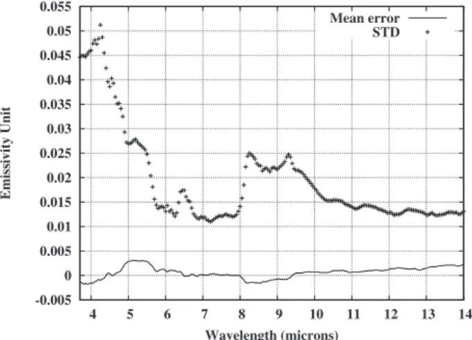
Theoretical simulations have been carried out in order to evaluate the standard deviation of the IASI-MSM approach. They are composed of a randomly selected atmospheric situation from the TIGR database and an emissivity spectrum from the 165-MOD-AST emissivity database. Then, a surface temperature is generated as the sum of the temperature of the atmosphere at the lowest level and a random number with zero mean and a standard deviation of 4 K. This value of 4 K results from an examination of the 40-yr European Centre for Medium-Range Weather Forecasts (ECMWF) Re-Analysis data (over land at night). This ensures that 99% of the skin temperatures chosen are between Tair_ ground 2 12 K and Tair_ground 1 12 K. Corresponding IASI channel brightness temperatures are then calcu-lated using the 4A model, and the noise equivalent temperature (NEDT) is added to the resulting bright-ness temperatures in order to account for the IASI in-strument noise. The IASI-MSM algorithm is then applied to each of these simulated spectra, and the sur-face temperature and emissivity spectra are retrieved. Five thousand such simulations were performed. Figure 4 displays the mean and the standard deviation of the difference between the retrieved emissivity spectra and the true ones for this set of 5000 simulations (nadir viewing and surface pressure at 1013 hPa). The lowest standard deviations are observed for the atmospheric windows around 10.5–14 and 5.5–8 mm (0.01–0.015) and the highest at around 8–10 mm (0.02) and 4 mm (0.045) due to both the higher emissivity variability and the higher impact of errors in the description of the atmo-spheric situation observed. These results are consistent with obtained by Pe´quignot et al. (2008) for AIRS. However, the standard deviation at 4 mm obtained here (;0.045) is larger than that obtained from the AIRS simulations (0.03). This is due to the larger radiometric noise of IASI at shorter wavelengths. Actually, the IASI noise between 4.435 and 4.186 mm, for a typical tropical atmosphere, is greater than 1 K and is still above 0.5 K
for all wavelengths smaller than 4.5 mm. For the 5.5–8- and 10.5–14-mm bands, the emissivity standard deviation ranges from 0.01 to 0.015. The corresponding mean er-ror obtained for the surface temperature from these simulations is 20.1 6 1.3 K. This error is consistent with recent reported errors (Bosilovich 2006; Zhang et al. 2007; Li et al. 2011).
4. Application of the IASI-MSM data to
observations over the tropics: Comparison with MODIS and ECMWF forecast products a. Description of the data used for the comparisons
Three databases have been used for the purpose of comparing IASI retrievals with MODIS retrievals (surface temperature and emissivity) and with meteo-rological analyses–forecasts (surface temperature). The MODIS instrument operates on both the Terra and Aqua platforms. The MODIS Land Team provides global maps of land surface temperature and emissivity at 6 wavelengths, centered on 3.75, 3.96, 4.05, 8.55, 11.03, and 12.02 mm (corresponding to MODIS channels 20, 22, 23, 29, 31, and 32, respectively); at three temporal resolutions (daily, weekly and monthly); and at two spatial resolutions (0.018 and 0.058) for both night and day. For the purpose of comparing with the IASI-MSM products obtained here, nighttime, monthly data from the Terra platform have been used (MOD11C3 data, with a spatial resolution of 0.058), its local equatorial crossing time being closer to that of MetOp (approxi-mately 2130 UTC for Terra, 2130 UTC for MetOp, and 0130 UTC for Aqua). These land products are available FIG. 3. Example of a complete emissivity spectrum retrieval process. Emissivity is first estimated at each of the 101 hinge points (black squares). Then, the first-guess spectrum (in blue) is obtained from the 165-MOD-AST database through a least squares mini-mization method. Finally, the retrieved spectrum (in red) is ob-tained by a fitting procedure.
TABLE2. Mean and standard deviation of the spectral emis-sivity for the three channels selected for estimating the surface temperature obtained from the MODIS/UCSB and ASTER/JPL libraries. IASI channel (wavelength; mm) Mean emissivity Std dev of emissivity 754 (12.001) 0.975 0.012 867 (11.608) 0.971 0.013 921 (11.429) 0.970 0.013
for three versions: V4 (from 24 February 2000 until 31 December 2006), V4.1 (from 1 January 2007), and V5 (from 5 March 2000). The version V4.1 uses the re-trieval LST E algorithm of V4, with data inputs from the V5 (level-1B radiance data, geolocation data, cloud mask, atmospheric profiles, and land and snow cover data). This version was created in response to underestimation problems in the V5 Climate Modeling Grid (CMG) products. Recent validations reveal that the V5 CMG products underestimate surface temper-ature by up to 6 K, especially in desert and semiarid regions (Hulley and Hook 2009). In this study, com-parisons with MODIS are made with version V4.1. The data were downloaded online (https://wist.echo.nasa. gov/api/).
As mentioned in the introduction, the UW-BF emis-sivity database provides a global land surface emisemis-sivity dataset that combines moderate-spectral-resolution MODIS data (MOD11, version V4.1) and high-resolution laboratory spectra from the USCB and ASTER spectral libraries. The resulting spectrum is composed of 10 hinge points linked together by a linear interpolation (see Seemann et al. 2008).
IASI-MSM-retrieved land surface temperatures have also been compared with what ECMWF calls forecast products, available for T 1 3 h to T 1 72 h at 3-h in-tervals from base times 0000 and 1200 UTC (only the 0000 UTC base time was used here) on a 0.258 3 0.258 grid. To compare with the skin temperature retrieved from the IASI-MSM method, the forecast products have been interpolated to the IASI local equatorial crossing time (2130 UTC).
b. Surface temperature in the tropical band: Comparison with ECMWF forecast product and MODIS data
Figure 5 displays maps of the surface temperature from the IASI-MSM method, from MODIS, and from ECMWF forecast products (referred to as EC-FC in the following), for June and December 2008, for nighttime observations. Table 3 gives the mean and standard de-viations resulting from these comparisons. Comparisons with MODIS show a significant bias (21.4 K for June and 21.1 K for December) and a standard deviation of 1.4 K. The largest differences are mainly seen over the more arid regions, during summer. In winter, that is to say, June in the Southern Hemisphere and December in the Northern Hemisphere, the biases are both around 20.8 K with relatively good standard deviations of 1.0 K (June) and 1.4 K (December), respectively. The situa-tion is different in summer with a much higher bias (about 21.9 K) whereas the standard deviation remains acceptable (1.5 K in June and 1.3 K in December). This seasonal difference is likely to come from the difference in the overpass times of the two platforms (the local equatorial crossing time for Terra is 2230 UTC and that of MetOp is 2130 UTC) combined with the observed strong surface temperature diurnal cycle, negligible at that hour of the day in winter but still significant in summer with an impact of about 1.0 K, especially for arid surfaces (see, e.g., Pinker et al. 2007). The standard deviation of the differences is consistent with the theo-retical expected error determined in section 3b (1.3 K). The bias in the ECMWF forecasts is smaller (#0.3 K), but with a significant standard deviation, especially for December (2.2 K) where the EC-FC surface tempera-ture over the Sahara is significantly higher than those retrieved by either IASI-MSM or MODIS. In general, EC-FC temperatures are warmer than IASI-MSM and MODIS temperatures. Finally, it should be emphasized that the IASI-MSM results lie in between those from MODIS and from ECMWF; moreover, the bias and standard deviation are consistent with recently reported errors on surface temperature estimations (Wan 2003; Wan et al. 2004; Bosilovich 2006; Zhang et al. 2007). c. IASI infrared surface emissivity spectrum and
comparison with UW-BF and MODIS data over selected regions in Africa
Comparisons are made with the MODIS/Terra monthly mean emissivity product given at six wave-lengths (3.75, 3.96, 4.05, 8.55, 11.03, and 12.02 mm) and with the continuous emissivity spectra derived from these measurements and obtained from the UW-BF method. Following Pe´quignot et al. (2008), these FIG. 4. Mean and standard deviation of the difference between
the retrieved emissivity spectrum and the true outcome for a set of 5000 simulations (nadir viewing, surface pressure at 1013 hPa). The standard deviation provides an estimate of the IASI-MSM-expected standard deviation.
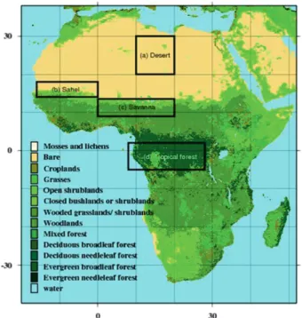
comparisons are made for four regions in Africa selected for their good land-cover-type homogeneity and corre-sponding to the main type of surface encountered in Africa: desert, Sahel, savanna, and tropical forest (see Fig. 6). For each region, the IASI-MSM data have been applied to the IASI observations for June. The resulting spatially averaged IASI-MSM emissivity spectra (from 3.7 to 14.0 mm at a 0.05-mm resolution) are displayed in Fig. 7 (in red). Also plotted in Fig. 7 are the spatially averaged emissivity spectra extracted from the UW-BF dataset for the same month (in black). The spatially averaged emissivities of the six MODIS V4.1 channels are also shown in blue. In general, the spectra obtained by the IASI-MSM simulations are consistent with the MODISV4.1 and the UW-BF products. For the differ-ent products compared here, the quartz Reststrahlen bands at 8.5 and 4 mm dominate the spectra for arid or
semiarid regions (desert, Sahel, and to a lesser extent savanna). This is explained by the fact that quartz dominates the mineralogical composition of the earth soils. In these bands, emissivity increases with vegeta-tion (and soil moisture); for example, no such bands can be seen for the tropical forest. In general, the different methods agree well in the 8–9.5-mm band, with a mean difference lower than 0.02. It is, however, worth pointing out that the IASI-MSM method actually reproduces the local maximum of emissivity at 8.65 mm observed in the high spectral resolution laboratory spectra within the 165-MOD-AST emissivity libraries for sandy soil. On the contrary, MODIS, with only one channel centered at 8.55 mm, cannot reproduce the high variability of this spectral region. At 4 mm the differences are greater than at longer wavelengths, in general between 0.02 and 0.04. These larger discrepancies are consistent with the
TABLE3. Mean and standard deviation for the differences (K) in MODIS 2 IASI-MSM and EC-FC 2 IASI. For MODIS, the bias and standard deviation are also given by hemisphere.
MODIS 2 IASI EC-FC 2 IASI
June 2008 21.4 61.4 Northern Hemisphere 22.0 61.5 0.3 61.6 Southern Hemisphere 20.8 61.0
December 2008 21.1 61.4 Northern Hemisphere 20.8 61.4 0.2 62.2 Southern Hemisphere 21.9 61.3
FIG. 5. Monthly mean surface temperature (K) at night from (top) IASI (this study), (middle) MODIS V4.1, and (bottom) the ECMWF forecast product for (left) June and (right) December 2008.
standard deviation expected theoretically in this spectral region (see section 3b). The differences obtained at 11 and 12 mm, on the order of 0.02 for Sahel and savanna, are more surprising since the theoretical error for this
spectral region is expected to be less than 0.015. How-ever, it should be noted that, for cases where discrep-ancies are significant, the MODISV4.1 and UW-BF emissivity values (also based on the V4.1) are close to 0.95, which is quite a low value for this spectral region and not consistent with values found in the 165-MOD-AST database that is supposed to contain many of the surface emissivities that exist on Earth: the averaged values of the emissivity in this database are, however, 0.970 6 0.013 at 11 mm and 0.975 6 0.012 at 12 mm (see Fig. 1).
d. Monthly mean land surface emissivity: Seasonal variations
Figure 8 displays emissivity over the tropical band at three wavelengths—3.8, 8.55, and 12.0 mm—for four months during 2008, corresponding to the four seasons: January, April, July, and October. The variations ob-served are highly dependent on the type of surface as well as on the wavelength considered. Emissivity at 12.0 mm is not sensitive to the season whatever the re-gion is. This result is consistent with the small standard deviation of the emissivity observed in laboratory spectra at these wavelengths (see Fig. 1), showing that they are not sensitive to the soil or vegetation types. At 3.8 and 8.55 mm, two wavelengths situated in the two quartz Reststrahlen bands, the amplitude of the varia-tions depends on the characteristics of the surface con-sidered. For arid regions, the seasonal variations are relatively small. This can be explained by the fact that FIG. 6. Geographical area covered by the four African regions
studied: desert, Sahel, savanna, and tropical forest, labeled with a– d, respectively [surface-type classification from the 8-km global land cover classification of DeFries et al. (1998)].
FIG. 7. The IR emissivity spectra for the month of June 2008 for the four regions in Fig. 6: (a) desert, (b) Sahel, (c) savanna, and (d) tropical forest. The emissivity spectrum calculated by the IASI-MSM is shown in red. The emissivity spectrum from UW-BF database is shown in black. The six MODIS emissivities at 3.75, 3.96, 4.05, 8.55, 11.03, and 12.02 mm from version V4.1 are shown in blue.
the soil characteristics remain similar for all seasons, mainly constituted of sandy quartz with no vegetation. For regions with vegetation, which are more sensitive to the season [i.e., to the precipitations and to the soil mois-ture; Salisbury and D’Aria (1992); Che´din et al. (2004)], emissivity seasonal variations are more important and can reach 0.05. Around the equator, the seasonal cycle is very small, as is to be expected in such a region. To analyze these variations in more detail, Fig. 9 displays time series from July 2007 to December 2010 of (i) emis-sivity in the two Reststrahlen bands (3.8 and 8.55 mm), (ii) the normalized difference vegetation index (NDVI) de-rived from MODIS (Miura et al. 2000; Huete et al. 2002), (iii) global monthly precipitation results [available from the Global Precipitation Climatology Project (Adler et al. 2003) only until September 2009], and (iv) soil moisture derived from Advanced Very High Resolution Radiometer (AVHRR) data (Njoku et al. 2003). All of these data were extracted online (http:// gdata1.sci.gsfc.nasa.gov/daac-bin/G3/gui.cgi?instance_ id5neespi). These variations are shown for the four regions described in Fig. 6: desert, Sahel, savanna, and
tropical forest. For Sahel, the emissivity at 8.55 mm displays variations with amplitude of about 0.05, strongly correlated with the NDVI and the soil moisture. Following the vegetation development, the emissivity maximum occurs in September after a growing season starting in May (corresponding to the wet season); on the contrary, during the dry season (from December to May), emissivity remains low and stable. This pattern of behavior over the Sahel is well known and has been described in several studies (e.g., Jarlan et al. 2008). At 3.8 mm, the maxima also occur in September, but the emissivity exhibits a secondary maximum in January that is not correlated with NDVI or to the amount of precipitation. However, it seems to correspond to a small local maximum in the soil moisture that would tend to increase the emissivity. However, this correla-tion has to be considered carefully, given the standard deviation of the retrieval at these wavelengths (about 0.04). For savanna, the seasonal cycle obtained for the two wavelengths is similar and follows that observed for Sahel, with a maximum of emissivity in September, corresponding to the end of the growing season and with FIG. 8. Seasonal variations of the land surface emissivity at (left to right) three selected wavelengths: 3.8, 8.55, and 12.0 mm, for four
an emissivity minimum just before the beginning of the emergence of the vegetation, in May. However, for this region, the amplitude is less significant (,0.04), which is likely due to the soil moisture that remains significant throughout the year (greater than 0.1 g cm3), since the emissivity in the Reststrahlen band is mainly sensitive to the humidity of the surface. For the tropical forest, emissivity does not exhibit a seasonal cycle. The amount of vegetation and humidity is high over all seasons, leading to an almost constant value of the emissivity. Finally, concerning the desert, even though emissivity variations are not expected for this type of surface, a weak seasonal cycle is observed at 8.55 mm (ampli-tude , 0.03). We attribute these variations to a possible remaining contamination by aerosols, in particular low aerosols, which are not completely detected by our cloud–aerosol screening algorithm. Indeed, the summer season over the Sahara corresponds to a large emission of dust particles (Schepanski et al. 2007; Klose et al. 2010). A large number of the aerosol-contaminated scenes are removed from the retrieval by the use of the clear-sky screening algorithm described in section 2d, but a small amount may not have been detected. It is worth pointing out that this error remains small regarding the
standard deviation of the emissivity expected in this spec-tral region. Nevertheless, improvements to the aerosol– cloud mask are being developed to remove these aerosol residuals from the emissivity retrieval.
5. Application of the IASI-MSM at the local scale: The MEVEX Oman campaign
To go further into the validation of the MSM ap-proach, IASI-retrieved emissivities are here compared with those derived from the Airborne Research In-terferometer Evaluation System (ARIES). The ARIES interferometer is flown on the Facility for Airborne Atmospheric Measurements (FAAM) BAe 146–301 Atmospheric Research Aircraft and is capable of recording infrared radiances in the spectral range 18– 3.3 mm at a spectral resolution of 1 cm21 with a data acquisition rate of 4 Hz (Wilson et al. 1999). Using ARIES has the advantage that, during low-level flights, the surface emissivity can be derived directly from the hyperspectral data (Newman et al. 2005; Thelen et al. 2009). Data were collected during the Middle East Validation Experiment (MEVEX) campaign in the re-gion of Oman in May 2009.
FIG. 9. Seasonal variation of emissivity at 3.8 mm (red curves) and 8.55 mm (green curves) from July 2007 to December 2010 for the regions defined in Fig. 6: (a) desert, (b) Sahel, (c) savanna, and (d) tropical forest; as well as a comparison with NDVI (right axis; black curves), monthly precipitations in millimeters per month (bottom figures, left axis; blue curves), and soil moisture in grams per centimeter cubed (bottom, right axis; blue rectangles). Monthly precipitation results are only available until September 2009.
a. MEVEX Oman campaign May 2009
The ARIES interferometer has the ability to view both upwelling and downwelling radiances. Thelen et al. (2009) demonstrate that it is possible to separate the (spectrally varying) downwelling emission reflected by the surface from the (relatively spectrally smooth) sur-face emission and, thereby, estimate both the sursur-face temperature and spectral emissivity. This method has been slightly modified over land, where the reflected atmospheric emission due to ozone around 1050 cm21 is used to infer the proportion of downwelling rays re-flected at the surface. During the MEVEX campaign in Oman in May 2009, two flights with low-level aircraft transects were selected as suitable for emissivity re-trieval from ARIES. These took place over the coast and interior of the Oman region, which corresponds to a desert area.
b. ARIES–IASI-MSM emissivity comparisons Figure 10 displays comparisons between ARIES emissivity at 9 mm (colored squares) for the two flights of the MEVEX Oman campaign in May 2009 and the IASI-MSM emissivity for the whole month (colored stars). Figure 10 brings into evidence the good agree-ment between the two products obtained from two quite different approaches. It also emphasizes the large spatial variations experienced by emissivity at very local scales: for example, over an area of less than 0.58, emissivity
variations can be as large as 0.1, resulting from surface property changes. This result shows the utility of the IASI-MSM approach, which allows high-spatial-resolution (a single IASI spot) emissivity retrievals to be carried out at the global scale. Figure 11 shows four examples of comparisons between ARIES and IASI-MSM spectra averaged over the four small areas of 0.38 3 0.38 delimited in Fig. 10 by the black rectangles. Averaged MODIS V4.1 data points are also shown. ARIES and IASI-MSM emissivities generally agree well, with differences smaller than 0.02 for the 10–14-mm band and at most of 0.05 in the Reststrahlen band at 8 mm; overall, the dif-ferences are smaller than 0.02. For the 10–14-mm band, however, even if the differences are small (less than 0.02), the bias observed between the two products is unexpected, with the IASI-MSM emissivity almost al-ways larger than those of ARIES. The low values ob-tained from ARIES are not consistent with values observed in the 165-MOD-AST emissivity libraries (see also section 4c), leading to two possible explanations: either the ARIES emissivities are underestimated in this part of the spectrum (the estimated standard deviation in the ARIES retrievals is 60.015) or the kind of soil observed in the geographical region considered here is not represented in the 165-MOD-AST database. In the latter case, because the IASI-MSM method assumes an almost constant emissivity at 12 mm (0.97 with a stan-dard deviation less than 0.015), a surface with a true emissivity substantially smaller than this value would FIG. 10. Comparison between ARIES- and IASI-MSM-retrieved emissivities at 9 mm from the MEVEX
Oman campaign during May 2009. The small colored squares highlight ARIES emissivity retrievals along the flight tracks, and the colored stars correspond to the IASI-MSM emissivity retrievals for each IASI clear-sky nighttime location during May 2009 for flight (left) B445 (5 May) and (right) B446 (7 May). The large black squares are used in Fig. 11.
correspond to a retrieved value shifted by almost the difference between the true emissivity and the assumed one. In the same manner, in the case of an unusually wet surface, such as after a significant rainfall, Hulley et al. (2010) show that the emissivity at 11 and 12 mm can be increased by about 2% and 1.5%, respectively. With the hypothesis assumed here on the 12-mm channel, the emissivity of the whole spectrum could be under-estimated when considering only one IASI spot. To im-prove such simulations at very local scales, the hypothesis on the emissivity value used at 12 mm can be chosen more carefully by taking into account more precisely the properties of the surface considered (humidity, compo-sition, etc.). It should be noted that the resulting error remains on the same order of magnitude as the expected error estimated in section 3b. Nevertheless, for the comparisons considering here, it may be emphasized that the MODIS data points in general stand between the two other products.
6. Conclusions
High-spectral-resolution observations from IASI over the tropics (308N–308S) for the period July 2007–December
2010 have been interpreted in terms of monthly mean surface skin temperature and emissivity spectra at a resolution of 0.05 mm. The IASI-Multispectral Method approach developed for that purpose is derived from the method of Pe´quignot et al. (2008) for application to AIRS observations. Comparisons with MODIS (sur-face temperature and low-resolution emissivity avail-able at six wavelengths) and ECMWF forecasts (surface temperature) show the IASI-MSM surface tempera-ture and emissivity spectrum standard deviation to be consistent with the errors expected theoretically (0.01–0.015 at 10.5–14 and 5.5–8 mm, 0.025 at 8–9 mm, and 0.045 at 4 mm). For the surface temperature, a bias of 20.8 K (61.3 K) is observed with MODIS in winter and of 21.9 K (61.4 K) in summer, for each hemi-sphere. This seasonal difference is likely to come from the difference in the local equatorial crossing times of the platforms MetOp (2130 UTC, IASI) and Terra (2230 UTC, MODIS) combined with the observed strong surface temperature diurnal cycle, negligible at that hour of the day in winter but still significant in summer with an impact of about 1.0 K, especially for arid sur-faces. The bias with the ECMWF forecast product is smaller (,0.3 K), but the standard deviation is larger, FIG. 11. Examples of comparisons between high-resolution spectra from ARIES and from IASI-MSM averaged
over the four correspondingly labeled areas in Fig. 10. Averaged ARIES spectra are depicted in red (pink dashed line for standard deviation) and averaged IASI-MSM emissivity spectra are depicted in blue (blue dashed line for standard deviation). Black symbols represent MODIS V4.1 emissivity.
especially for December (2.2 K instead of 1.6 K in June), when the forecast surface temperatures in the Sahara are higher than those retrieved by either IASI-MSM or MODIS. Note that the IASI-MSM surface temperatures lie in between these two different surface temperature products. Concerning the surface emissivity spectra, comparisons with MODIS/Terra data (six channels) or with MODIS-UW-BF data (continuous low-resolution spectra), for four regions in Africa with different vege-tation characteristics, show results in good agreement with the expected theoretical standard deviation. The quartz Reststrahlen bands at 8.5 and 4 mm dominate the spectra for arid regions and the results show that the IASI-MSM method satisfactorily reproduces these spectral regions with high emissivity variability as, for example, the local maximum seen at 8.65 mm in the laboratory spectra from the 165-MOD-AST emissivity libraries for sandy soil. On the contrary, MODIS, with only one channel centered at 8.55 mm in the 8–10-mm band, cannot reproduce such features. The differences obtained at 11 and 12 mm for the semiarid regions are somewhat more surprising, with MODIS and UW-BF emissivity values close to 0.95, a value smaller than the values observed in the 165-MOD-AST database, while the IASI-MSM emissivities are on the order of 0.97. At 3.8 and 8.55 mm, two wavelengths situated in the two quartz Reststrahlen bands, we observe a seasonal vari-ation of the emissivity, the amplitude of which depends on the characteristics of the surface considered. In par-ticular, for Sahel or savanna regions, with vegetation more sensitive to the season (i.e., to precipitation and soil moisture), the emissivity variations are more im-portant (up to 0.05) and can be directly related to the vegetation cycle. Finally, comparisons with emissivities derived from the Airborne Research Interferometer Evaluation System measurements, collected on board an aircraft flying at low altitude during the MEVEX campaign over Oman, show good agreement between the two sets of data. Spatial variations observed for the IASI-MSM emissivities are consistent with those de-rived from ARIES and the differences are, in general, on the order of 0.02 or less throughout the spectra. For some cases, however, IASI-MSM emissivities are greater than those from ARIES at 12 mm. There are two possible explanations for this discrepancy: either the ARIES emissivities are underestimated in this part of the spectrum or the type of soil observed in this geo-graphical region is not represented in the 165-MOD-AST database, leading to an overestimation of the IASI-MSM emissivity, due to our assumption of an emissivity value at 12 mm set to the 165-MOD-AST database aver-age value. A similar problem was observed for the Sahel region when compared with MODIS results (see Fig. 7).
Further investigations should be performed to un-derstand these differences, such as the use of additional sources of laboratory emissivity measurements in order to better constrain the emissivity properties of the re-gions considered, or a refinement of the assumption of a constant value of the emissivity at 12 mm. It must be pointed out that the differences observed are on the order of the standard deviation expected from this method. This result is important because it demonstrates the capability of the IASI-MSM approach to be applied to geographical regions where the emissivity shows fast spatial variations, as it is the case of Oman.
Acknowledgments. Airborne data were obtained us-ing the BAe-146-301 Atmospheric Research Aircraft (ARA) flown by Directflight, Ltd., and managed by FAAM, which is a joint entity of the Natural Environ-ment Research Council (NERC) and the Met Office. We are happy to thank R. Armante and L. Cre´peau for their help and for fruitful discussions. The authors also thank the reviewers for their comments that helped to improve the manuscript.
REFERENCES
Adler, R. F., and Coauthors, 2003: The version 2 Global Pre-cipitation Climatology Project (GPCP) monthly prePre-cipitation analysis (1979–present). J. Hydrometeor., 4, 1147–1167. Baldridge, A. M., S. J. Hook, C. I. Grove, and G. Rivera, 2009: The
ASTER spectral library version 2.0. Remote Sens. Environ., 113, 711–715.
Bosilovich, M. G., 2006: A comparison of MODIS land surface temperature with in situ observations. Geophys. Res. Lett., 33, L20112, doi:10.1029/2006GL027519.
Che´din, A., N. A. Scott, C. Wahiche, and P. Moulinier, 1985: The improved initialization inversion method: A high-resolution physical method for temperature retrievals from satellites of the TIROS-N series. J. Climate Appl. Meteor., 24, 128–144. ——, E. Pe´quignot, S. Serrar, and N. A. Scott, 2004: Simultaneous
determination of continental surface emissivity and tem-perature from NOAA 10/HIRS observations: Analysis of their seasonal variations. J. Geophys. Res., 109, D20110, doi:10.1029/2004JD004886.
Chevallier, F., F. Che´ruy, N. A. Scott, and A. Che´din, 1998: A neural network approach for a fast and accurate computation of a longwave radiative budget. J. Appl. Meteor., 37, 1385–1397. Crevoisier, C., A. Che´din, S. Heilliette, N. A. Scott, S. Serrar, and
R. Armante, 2003: Mid-tropospheric CO2 retrieval in the
tropical zone from airs observations. Proc. 13th Int. TOVS Study Conf., Ste. Adele, QC, Canada, Int. TOVS Working Group. DeFries, R., M. Hansen, J. R. G. Townshend, and R. Sohlberg,
1998: Global land cover classifications at 8km spatial resolu-tion: The use of training data derived from Landsat imagery in decision tree classifiers. Int. J. Remote Sens., 19, 3141–3168. French, A., T. Schmugge, J. Ritchie, A. Hsu, F. Jacob, and
K. Ogawa, 2008: Detecting land cover change at the Jornada Experimental Range, New Mexico, with ASTER emissivities. Remote Sens. Environ., 112, 1730–1748.
Gillespie, A., S. Rokugawa, T. Matsunaga, J. S. Cothern, S. Hook, and A. B. Kahle, 1998: A temperature and emissivity separa-tion algorithm for Advanced Spaceborne Thermal Emission and Reflection Radiometer (ASTER) images. IEEE Trans. Geosci. Remote Sens., 36, 1113–1126.
Hook, S. J., A. R. Gabell, A. A. Green, and P. S. Kealy, 1992: A comparison of techniques for extracting emissivity in-formation from thermal infrared data for geologic studies. Remote Sens. Environ., 42, 123–135.
Huete, A., K. Didan, T. Miura, E. P. Rodriguez, X. Gao, and L. G. Ferreira, 2002: Overview of the radiometric and biophysical performance of the MODIS vegetation indices. Remote Sens. Environ., 83, 195–213.
Hulley, G. C., and S. J. Hook, 2009: Intercomparison of versions 4, 4.1 and 5 of the MODIS land surface temperature and emis-sivity products and validation with laboratory measurements of sand samples from the Namib Desert, Namibia. Remote Sens. Environ., 113, 1313–1318.
——, ——, and A. M. Baldridge, 2008: ASTER Land Surface Emissivity Database of California and Nevada. Geophys. Res. Lett., 35, L13401, doi:10.1029/2008GL034507.
——, ——, and ——, 2010: Investigating the effects of soil moisture on thermal infrared land surface temperature and emissivity using satellite retrievals and laboratory measurements. Remote Sens. Environ., 114, 1480–1493.
Jacquinet-Husson, N., and Coauthors, 2011: The 2009 edition of the GEISA spectroscopic database. J. Quant. Spectrosc. Ra-diat. Transfer, 112, 2395–2445.
Jarlan, L., S. Mangiarotti, E. Mougin, P. Mazzega, P. Hiernaux, and V. L. Dantec, 2008: Assimilation of spot/vegetation NDVI data into a Sahelian vegetation dynamics model. Remote Sens. Environ., 112, 1381–1394.
Jime´nez, C., J. Catherinot, C. Prigent, and J. Roger, 2010: Relations between geological characteristics and satellite-derived in-frared and microwave emissivities over deserts in northern Africa and the Arabian Peninsula. J. Geophys. Res., 115, D20311, doi:10.1029/2010GL042816.
Klose, M., Y. Shao, M. K. Karremann, and A. H. Fink, 2010: Sahel dust zone and synoptic background. Geophys. Res. Lett., 37, L09802, doi:10.1029/2010JD013959.
Li, J., J. Li, E. Weisz, and D. K. Zhou, 2007: Physical retrieval of surface emissivity spectrum from hyperspectral infrared radiances. Geophys. Res. Lett., 34, D01304, doi:10.1029/ 2007GL030543.
——, Z. Li, X. Jin, T. J. Schmit, L. Zhou, and M. D. Goldberg, 2011: Land surface emissivity from high temporal resolution geo-stationary infrared imager radiances: Methodology and sim-ulation studies. J. Geophys. Res., 116, D01304, doi:10.1029/ 2010JD014637.
Miura, T., A. Huete, and H. Yoshioka, 2000: Evaluation of sensor calibration uncertainties on vegetation indices for MODIS. IEEE Trans. Geosci. Remote Sens., 38, 1399–1409.
Nerry, F., J. Labed, and M.-P. Stoll, 1988: Emissivity signatures in the thermal IR band for remote sensing: Calibration procedure and method of measurement. Appl. Opt., 27, doi:10.1364/ AO.27.000758.
Newman, S. M., J. A. Smith, M. D. Glew, S. M. Rogers, and J. P. Taylor, 2005: Temperature and salinity dependence of sea surface emissivity in the thermal infrared. Quart. J. Roy. Meteor. Soc., 131, 2539–2557.
Njoku, E. G., T. L. Jackson, V. Lakshmi, T. Chan, and S. V. Nghiem, 2003: Soil moisture retrieval from AMSR-E. IEEE Trans. Geosci. Remote Sens., 41, 215–229.
Ogawa, K., T. Schmugge, F. Jacob, and A. French, 2003: Estima-tion of land surface window (8–12 mm) emissivity from multi-spectral thermal infrared remote sensing—A case study in a part of Sahara Desert. Geophys. Res. Lett., 30, 1067, doi:10.1029/ 2002GL016354.
Pe´quignot, E., A. Che´din, and N. A. Scott, 2008: Infrared conti-nental surface emissivity spectra retrieved from AIRS hy-perspectral sensor. J. Appl. Meteor. Climatol., 47, 1619–1633. Pinker, R. T., D. Sun, M. Miller, and G. J. Robinson, 2007: Diurnal cycle of land surface temperature in a desert encroachment zone as observed from satellites. Geophys. Res. Lett., 34, L11809, doi:10.1029/2007GL030186.
Plokhenko, Y., and W. P. Menzel, 2000: The effects of surface re-flection on estimating the vertical temperature–humidity dis-tribution from spectral infrared measurements. J. Appl. Meteor., 39, 3–14.
Prabhakara, C., and G. Dalu, 1976: Remote sensing of surface emis-sivity at 9 mm over the globe. J. Geophys. Res., 81, 3719–3724. Salisbury, J. W., and D. M. D’Aria, 1992: Emissivity of terrestrial
materials in the 8–14 mm atmospheric window. Remote Sens. Environ., 42, 83–106.
——, and ——, 1994: Thermal-infrared remote sensing and Kirchhoff’s law 1. Laboratory measurements. J. Geophys. Res., 99 (B6), 11 897–11 911.
Schepanski, K., I. Tegen, B. Laurent, B. Heinold, and A. Macke, 2007: A new Saharan dust source activation frequency map derived from MSG–SEVIRI IR-channels. Geophys. Res. Lett., 34, L18803, doi:10.1029/2007GL030168.
Scott, N. A., and A. Che´din, 1981: A fast line-by-line method for atmospheric absorption computations: The automatized at-mospheric absorption atlas. J. Appl. Meteor., 20, 802–812. ——, and Coauthors, 1999: Characteristics of the TOVS Pathfinder
Path-B dataset. Bull. Amer. Meteor. Soc., 80, 2679–2701. Seemann, S. W., E. E. Borbas, R. O. Knuteson, G. R. Stephenson,
and H.-L. Huang, 2008: Development of a global infrared land surface emissivity database for application to clear sky sounding retrievals from multispectral satellite radiance mea-surements. J. Appl. Meteor. Climatol., 47, 108–123.
Stubenrauch, C. J., W. B. Rossow, F. Che´ruy, A. Che´din, and N. A. Scott, 1999: Clouds as seen by satellite sounders (3I) and imagers (ISCCP). Part I: Evaluation of cloud parameters. J. Climate, 12, 2189–2213.
Susskind, J., and J. Blaisdell, 2008: Improved surface parameter retrievals using AIRS/AMSU data. Algorithms and Technol-ogies for Multispectral, Hyperspectral, and Ultraspectral Im-agery XIV, S. S. Shen and P. E. Lewis, Eds., International Society for Optical Engineering (SPIE Proceedings Vol. 6966), doi:10.1117/12.774759.
Thelen, J.-C., S. Havemann, S. M. Newman, and J. P. Taylor, 2009: Hyperspectral retrieval of land surface emissivities us-ing ARIES. Quart. J., Roy. Meteor. Soc., 135, 2110–2124. Vaughan, R. G., W. M. Calvin, and J. V. Taranik, 2003: SEBASS
hyperspectral thermal infrared data: Surface emissivity mea-surement and mineral mapping. Remote Sens. Environ., 85, 48–63.
Wahiche, C., N. A. Scott, and A. Che´din, 1986: Cloud detection and cloud parameters retrievals from the satellites of the TIROS-N series. Ann. Geophys., 43, 207–222.
Wan, Z., 2003: Land surface temperature measurements from EOS MODIS data. NASA Contract NAS5-31370, 18 pp.
——, 2008: New refinements and validation of the MODIS land-surface temperature/emissivity products. Remote Sens. Envi-ron., 112, 59–74.
——, and Z. L. Li, 1997: A physics-based algorithm for retrieving land-surface emissivity and temperature from EOS/MODIS data. IEEE Trans. Geosci. Remote Sens., 35, 980–996. ——, D. Ng, and J. Dozier, 1994: Spectral emissivity measurements
of land-surface materials and related radiative transfer simu-lations. Adv. Space Res., 14, 91–94.
——, Y. Zhang, Q. Zhang, and Z. L. Li, 2004: Quality assessment and validation of the MODIS global land surface tem-perature. Int. J. Remote Sens., 25, 261–274.
Wilson, S. H. S., N. C. Atkinson, and J. A. Smith, 1999: The development of an airborne infrared interferometer for meteorological sounding studies. J. Atmos. Oceanic Technol., 16, 1912–1927.
Zhang, Y., W. B. Rossow, and P. W. Stackhouse, 2007: Comparison of different global information sources used in surface radi-ative flux calculation: Radiradi-ative properties of the surface. J. Geophys. Res., 112, D01102, doi:10.1029/2005JD007008. Zhou, D. K., A. M. Larar, X. Liu, W. L. Smith, L. L. Strow, P. Yang,
P. Schlu¨ssel, and X. Calbet, 2011: Global land surface emis-sivity retrieval from satellite ultraspectral IR measurements. IEEE Trans. Geosci. Remote Sens., 49, 1277–1290.
Zhou, L., R. E. Dickinson, Y. Tian, M. Jin, K. Ogawa, H. Yu, and T. Schmugge, 2003: A sensitivity study of climate and energy balance simulations with use of satellite-derived emissivity data over northern Africa and the Arabian Penin-sula. J. Geophys. Res., 108, 4795, doi:10.1029/2003JD004083.