Operational climate monitoring from space: the EUMETSAT satellite application facility on climate monitoring (CM-SAF)

(1)

HAL Id: hal-00304149

https://hal.archives-ouvertes.fr/hal-00304149

Submitted on 8 May 2008

HAL is a multi-disciplinary open access

archive for the deposit and dissemination of sci-entific research documents, whether they are pub-lished or not. The documents may come from teaching and research institutions in France or abroad, or from public or private research centers.

L’archive ouverte pluridisciplinaire HAL, est destinée au dépôt et à la diffusion de documents scientifiques de niveau recherche, publiés ou non, émanant des établissements d’enseignement et de recherche français ou étrangers, des laboratoires publics ou privés.

Operational climate monitoring from space: the

EUMETSAT satellite application facility on climate

monitoring (CM-SAF)

J. Schulz, P. Albert, H.-D. Behr, D. Caprion, H. Deneke, S. Dewitte, B. Dürr,

P. Fuchs, A. Gratzki, P. Hechler, et al.

To cite this version:

J. Schulz, P. Albert, H.-D. Behr, D. Caprion, H. Deneke, et al.. Operational climate monitoring from space: the EUMETSAT satellite application facility on climate monitoring (CM-SAF). Atmospheric Chemistry and Physics Discussions, European Geosciences Union, 2008, 8 (3), pp.8517-8563. �hal-00304149�

(2)

ACPD

8, 8517–8563, 2008 Operational climate monitoring from space: CM-SAF J. Schulz et al. Title Page Abstract Introduction Conclusions References Tables Figures ◭ ◮ ◭ ◮ Back Close

Full Screen / Esc

Printer-friendly Version Interactive Discussion

Atmos. Chem. Phys. Discuss., 8, 8517–8563, 2008 www.atmos-chem-phys-discuss.net/8/8517/2008/ © Author(s) 2008. This work is distributed under the Creative Commons Attribution 3.0 License.

Atmospheric Chemistry and Physics Discussions

Operational climate monitoring from

space: the EUMETSAT satellite

application facility on climate monitoring

(CM-SAF)

J. Schulz1, P. Albert1, H.-D. Behr1, D. Caprion2, H. Deneke3, S. Dewitte2, B. D ürr4, P. Fuchs1, A. Gratzki1, P. Hechler1, R. Hollmann1, S. Johnston5, K.-G. Karlsson5, T. Manninen6, R. M üller1, M. Reuter1, A. Riihel ä6, R. Roebeling3, N. Selbach1, A. Tetzlaff5, W. Thomas1, M. Werscheck1, E. Wolters3, and A. Zelenka4

1

Deutscher Wetterdienst (DWD), D-63004 Offenbach, P.O. Box 10 04 65, Germany

2

Royal Meteorological Institute of Belgium (RMI), Ringlaan 3 Avenue Circulaire B-1180 Brussels, Belgium

3

Koninklijk Nederlands Meteorologisch Instituut (KNMI), Wilhelminalaan 10 3732 GK De Bilt, The Netherlands

4

MeteoSchweiz, P.O. Box 514, CH-8044 Z ¨urich, Switzerland

5

Swedish Meteorological and Hydrological Institute (SMHI), Folkborgsv ¨agen 1 SE-601 76 Norrk ¨oping, Sweden

6

Finnish Meteorological Institute (FMI), P.O. BOX 503, FIN-00101 Helsinki, Finland Received: 29 February 2008 – Accepted: 2 April 2008 – Published: 8 May 2008 Correspondence to: J. Schulz (joerg.schulz@dwd.de)

(3)

ACPD

Full Screen / Esc

Abstract

The Satellite Application Facility on Climate Monitoring (CM-SAF) aims at the provi-sion of satellite-derived geophysical parameter data sets suitable for climate monitor-ing. CM-SAF provides climatologies for Essential Climate Variables (ECV), as required by the Global Climate Observing System implementation plan in support of the UN-5

FCCC. Several cloud parameters, surface albedo, radiation fluxes at the top of the atmosphere and at the surface as well as atmospheric temperature and humidity prod-ucts form a sound basis for climate monitoring of the atmosphere. The prodprod-ucts are categorized in monitoring data sets obtained in near real time and data sets based on carefully intercalibrated radiances. The CM-SAF products are derived from several 10

instruments on-board operational satellites in geostationary and polar orbit, i.e., the Meteosat and NOAA satellites, respectively. The existing data sets will be continued using data from the instruments on-board the new EUMETSAT Meteorological Op-erational satellite (MetOP). The products have mostly been validated against several ground-based data sets both in situ and remotely sensed. The accomplished accuracy 15

for products derived in near real time is sufficient to monitor variability on diurnal and seasonal scales. Products based on intercalibrated radiance data can also be used for climate variability analysis up to inter-annual scale. A central goal of the recently started Continuous Development and Operations Phase of the CM-SAF (2007–2012) is to further improve all CM-SAF data sets to a quality level that allows for studies of 20

inter-annual variability.

1 Introduction

Concerns about the Earth’s climate implicate an increasing necessity for climate moni-toring on a global scale. Only space-based observations can deliver the needed global coverage with sufficient quality and timeliness. Particularly over the ocean and sparsely 25

(4)

espe-ACPD

Full Screen / Esc

cially the operational meteorological satellites, now provide sufficiently long data series for climate analysis. Satellite data provide information on the climate system that are not available or difficult to measure from the Earths surface like top of atmosphere ra-diation, cloud properties or humidity in the upper atmosphere the two latter having a large impact on the greenhouse effect.

5

Understanding the processes that control the natural stability and variability of the climate system is one of the most difficult and challenging scientific problems faced by the climate science community today. An improved understanding of the interaction processes between water vapour and clouds as well as their radiative impact is urgently required.

10

The Earth’s Radiation Budget (ERB) is the balance between the incoming radiation from the sun and the outgoing reflected and scattered solar radiation plus the thermal infrared emission to space. Earth surface conditions greatly influence the radiation budget, e.g. through surface temperature variations in the thermal infrared and through a critical contribution to the planetary albedo (especially for desert regions and snow-15

and ice-covered polar regions).

Water vapour is a major greenhouse gas and is usually considered to play an am-plifying role in global warming through a strongly positive climate feedback loop (Held

and Soden,2000), although with some remaining question marks concerning the link to cloud feedback processes. Due to the non linearity of interactions between the radi-20

ation field and water vapour, outgoing longwave radiation (OLR) is more sensitive to a small humidity perturbation in a dry environment than in a moist region. For instance, increasing the upper tropospheric humidity from 5% to 10% at constant temperature, increases the outgoing longwave radiation by 10 Wm−2while increasing the upper tro-pospheric humidity from 25% to 30% only modifies OLR by less than 5 Wm−2. This 25

confers a central role to the dry upper troposphere regions in the radiation budget and its sensitivity. Documenting the recent decades history of the water vapour field should give some understanding of the mechanisms at play in the climate and how it responds to the increasing greenhouse gas concentration. For instance, the question: Will a

(5)

dry-ACPD

Full Screen / Esc

ing of the upper troposphere occur as CO₂increases, as postulated in recent climate change theory, or not? can be investigated with an extensive documentation of the tropospheric humidity from satellite (Rind,1998;Soden,2000).

Because the water vapour distribution results from the large scale dynamics and associated transports that take place at synoptic scales, its documentation can also 5

yield some insights into the dynamics of the atmosphere and its evolution. It is then important to monitor its evolution with high temporal resolution over a long time period. This effort could in principle be useful to detect, if any, trends not only in the mean climate but also in the transient activity, which is central to the energy cycle.

Clouds exert a blanketing effect similar to that of water vapour. In the infrared spectral 10

region clouds behave like black bodies, and emit radiation back to the Earth and to outer space depending on their temperature. As water vapour, clouds absorb and emit infrared radiation and thus contribute to the warming of the Earth’s surface. However, this effect is counterbalanced by the reflection of clouds, which reduces the amount of incoming solar radiation at the Earth’s surface. Because most clouds are bright 15

reflectors they block much of the incoming solar radiation and reflect it back to space before it can be absorbed by the Earth surface or the atmosphere, which has a cooling effect on the climate system. The net average effect of the Earth’s cloud cover in the present climate is a slight cooling because the reflection of radiation more than compensates for the greenhouse effect of clouds.

20

One of the most problematic issues in studying clouds is their transient nature– they are continuously changing in space and time, which make them very difficult to both observe and simulate in models. This also explains why differences in cloud descrip-tions and cloud parameterizadescrip-tions between various climate models are responsible for a major part of the variation seen in climate model scenarios through cloud feedback 25

processes (Stephens,2005). Hence, progress is needed here both concerning cloud observation and cloud modeling aspects.

From the above paragraphs it is obvious that a high quality combined water vapour– cloud– radiation time series derived from satellite data is of enormous value for climate

(6)

ACPD

Full Screen / Esc

research. This is reflected in the choice of products of the Satellite Application Facility on Climate Monitoring (CM-SAF). The CM-SAF is part of EUMETSAT’s SAF Network, that comprises eight SAFs (see www.eumetsat.int for further details). The SAF network is a network of networks, dedicated to tackle the tasks and challenges in the field of meteorology and climatology supported by satellite data as the main input. The CM-5

SAF as part of this network plays a major role in EUMETSAT’s activities towards climate monitoring.

Beside the issues of monitoring and understanding the climate system, adaptation to and active protection against climate change is highly relevant to societies. Both are strongly coupled to the production of electricity, where solar energy systems provide a 10

sustainable and environmentally sound alternative to traditional power plants. Accurate solar irradiance data is needed for the efficient planning and design of solar energy systems. CM-SAF radiation data may help to increase the efficiency of such systems, which leads to a potential reduction of CO₂ emissions by the replacement of fossil power plants.

15

This paper introduces the CM-SAF concept, its current products including their qual-ity and its near future plan. In the next section the historic background and the ob-jectives of CM-SAF are described in more detail. This is followed by a description of the individual climate monitoring products including the techniques to derive them and estimations of achieved accuracy. The last section is dedicated to the tasks of the so 20

called Continuous Development and Operations Phase (CDOP) with a duration of five years (2007–2012).

2 Background and objectives

First attempts to generate long-term data series of atmospheric quantities derived from satellite measurements go back to the early eighties when the International Satellite 25

Cloud Climatology Project (ISCCP) started its work (Rossow and Garder,1993). The cloud information from the ISCCP data set was successfully used to derive a

(7)

clima-ACPD

Full Screen / Esc

tology of the shortwave radiation budget (Gupta et al.,1999). Precursory cloud data sets are e.g., the PATMOS data set (Jacobowitz et al., 2003), the SCANDIA cloud climatology (Karlsson,2003) over Scandinavia, and the European Cloud Climatology

(Meerk ¨otter et al.,2004), which were all derived from Advanced Very High Resolution

Radiometer (AVHRR) observations. SCANDIA has recently been used to elucidate 5

possible weaknesses of regional climate simulations with respect to the simulation of cloud amount, cloud optical thickness and the vertical distribution of clouds (Karlsson

et al.,2007). The NASA Water vapour Project (NVAP) provides global total column wa-ter vapour data sets derived from Television and Infrared Operational Satellite (TIROS) Operational Vertical Sounders (TOVS), and Special Sensor Microwave/Imager (SSM/I) 10

data spanning a period over 14 years (1998–2001)(Vonder Haar,2003).

Although accuracy and precision of satellite-based time series may locally be lower than existing and corresponding data sets derived from ground-based measurements, they provide a much more homogeneous data quality compared to the heterogeneous observation systems at the ground. However, dedicated effort is needed to generate 15

homogeneous, stable and accurate data sets with high spatial resolution from recent, current and future satellite sensors. Then, such time series of satellite-derived quan-tities can be used e.g., for the detection of climate change. Following the terminology of the NOAA White Paper on creating Climate Data Records (CDRs) from satellite measurements (Colton et al., 2003), CM-SAF has the mandate to generate thematic 20

climate data records in an operational off-line environment. This requires a very accu-rate absolute calibration as well as very high sensor stability over time (Ohring et al.,

2005). Additionally, radiance data coming from different satellite platforms must be in-tercalibrated. It is required that these data sets and related methods are provided by several satellite operators.

25

Within the range of essential climate variables as defined in the GCOS Second Adequacy Report (GCOS, 2003) the CM-SAF currently focuses on the provision of geophysical parameters describing elements of the energy and water cycle. CM-SAF provides regional products with comparably high spatial resolution as well as global

(8)

ACPD

Full Screen / Esc

products that complement ongoing international activities. CM-SAF exploits the po-lar orbiting NOAA and MetOp satellites utilizing data from the Advanced Very High Resolution Radiometer (AVHRR), High resolution Infrared Radiation Sounder (HIRS), Infrared Atmospheric Sounding Interferometer (IASI), Advanced Microwave Sounding Unit (AMSU) and Microwave Humidity Sounder (MHS) instruments. Additionally, the 5

Global Earth Radiation Budget (GERB) (Harries et al., 2005) and the Spinning En-hanced Visible and Infrared Imager (SEVIRI) radiometers (Schmetz et al.,2002) on-board the METEOSAT Second Generation (MSG) satellites are used. Data from the Clouds and Earth’s Radiant Energy System (CERES) on-board TERRA and AQUA support the retrieval of radiation fluxes at top of the atmosphere. Furthermore, data 10

of the Special Sensor Microwave/Imager (SSM/I) series are used to provide a con-sistent time series of total column water vapour over the ocean spanning the period 1987–2005.

CM-SAF data sets can be categorized into three different groups fulfilling differ-ent requiremdiffer-ents. During the Initial Operations Phase (IOP, 2004–2007) operational 15

procedures to quickly process large amounts of data were established. Products are available in almost real time but retrieval schemes changed over time. Additionally, ra-diances used as input were only nominally calibrated, i.e., no intercalibration accounts for sensor changes and other sensor related errors. During the so called Continuous Development and Operations phase (CDOP, 2007–2012) the focus is on the genera-20

tion of long homogeneous time series of the CM-SAF products. The three data set categories and their properties are:

– CDRs for operational climate monitoring are constructed from so called

Environ-mental Data Records (EDR). EDRs are data sets containing instantaneous esti-mates of geophysical variables retrieved in near real time only utilizing information 25

from the past and aiming at a small random error. Input to this processing are nominal calibrated radiances or automatically intercalibrated sensor data if pro-vided by the space agencies. The instantaneous EDRs are then integrated over time to obtain daily and monthly averaged products. Within this process also

(9)

in-ACPD

Full Screen / Esc

formation from the future is used, e.g., a whole month of data is used to compute daily averages for a particular month employing also temporal correlations to fill gaps. The application area of these data sets is on diurnal and sub-seasonal to seasonal time scales, e.g., the monitoring of extreme events and the support of National Meteorological Services (NMSs) climate departments in early dissemi-5

nation of climate information to the public. Additionally, the products are accurate enough to be used for solar energy applications. The use of longer time scales depends on the quality of automated intersensor calibration. Derived geophysical averages may have to be corrected using ground based information for further use. The data sets currently created at CM-SAF mostly belong to this category. 10

– Reprocessed CDRs form a second class and will be created if substantial

knowl-edge on the correction of instrument and retrieval errors can be applied. This should at least include inter satellite homogenisation and frozen algorithms for the production of the data set. Depending on the number of satellite instruments involved in a product and the success of automated radiance homogenisation as 15

well as corrections of systematic errors caused by instrument failures or orbit vari-ations, the products are expected to be useful for time scales ranging from diurnal, seasonal to inter-annual. For the latter scale the variability is much smaller com-pared to diurnal and sub-seasonal fluctuations. Most of the CM-SAF products will reach this status during the CDOP.

20

– A third class of CDRs will be provided for the analyses of long term climate

vari-ability (decadal). Here it is necessary that expert teams have improved absolute calibration of the involved instruments to the highest possible level and that other instrument and orbit related systematic errors are diminished to a level that the very small decadal variability in a variable can be monitored. Some of the pa-25

rameters, e.g., total column water vapour over oceans from passive microwave imager data may reach this status shortly after the CDOP when the time series of such data approaches 30 years. Additionally, the records starting from new

(10)

instru-ACPD

Full Screen / Esc

ments as IASI and others on EUMETSAT MetOp satellite are expected to deliver such high quality data to create a data set suitable for the analysis of decadal variability.

3 Products, retrieval schemes and validation

As mentioned above CM-SAF focuses on retrieving geophysical parameters from satel-5

lite data employing inversion schemes based on radiation transfer theory. This com-plements other international activities on the use of satellite data in climate research as the use of radiance data for climate trend detection and the assimilation of satel-lite data into dynamical models to retrieve geophysical products as e.g. in the ERA-40 reanalysis. The products currently are:

10

– Cloud parameters: cloud fractional cover (CFC), cloud type (CTY), cloud top

pres-sure (CTP), cloud top height (CTH), cloud top temperature (CTT), cloud phase (CPH), cloud optical thickness (COT), cloud water path (CWP);

– Radiation budget parameters at the surface and at the top of the atmosphere

(TOA). Surface: Incoming short-wave radiation (SIS), surface albedo (SAL), net 15

shortwave radiation (SNS), net longwave radiation (SNL), downward (SDL) and outgoing longwave radiation (SOL), surface radiation budget (SRB); TOA: Incom-ing solar radiative flux (TIS), reflected solar radiative flux (TRS), emitted thermal radiative flux (TET);

– Humidity products: Total (HTW) and layered (HLW) precipitable water, mean

tem-20

perature, and relative humidity for 5 layers as well as specific humidity and tem-perature at the six layer boundaries (HSH).

These products were mainly discussed and defined during the development phase of the CM-SAF (Woick et al.,2002). The list of products reflects atmospheric parameters that can be derived from sensors on-board operational satellites with state-of-the-art 25

(11)

ACPD

Full Screen / Esc

retrieval schemes. The list was confirmed by a user survey held by CM-SAF in 2001 which allowed also to prioritize the development of products. The majority of prod-ucts is classified as essential climate variable (ECV), as can be seen in the GCOS implementation plan (GCOS,2004). Although well known parameters as sea and land surface temperature as well as ice and snow cover are not explicitly provided their im-5

pact is implicitly covered by surface albedo and surface radiation fluxes. All products are available via electronic ordering at www.cmsaf.eu.

Currently, all CM-SAF products derived from instruments on the Meteosat platform cover the full METEOSAT visible disc. Products derived from AVHRR measurements cover an area between 30◦N to 80◦N and 60◦W to 30◦E, i.e. basically Europe and 10

the Northeast Atlantic. Water vapour products derived from ATOVS data are provided with global coverage. Near real time monitoring products are available from May 2007 onwards. Additionally, a total column water vapour product derived from SSM/I data that covers global ice-free ocean areas is provided. The SSM/I record is based on intercalibrated SSM/I brightness temperatures (Andersson et al.,2007) and is available 15

for the period 1987–2005. Cloud products and surface albedo will be further extended to cover the Inner Arctic. AVHRR, ATOVS and IASI data from the MetOp satellite will be used to further improve coverage and accuracy of the products in the near future.

Most of the CM-SAF products are provided at a (15 km)2spatial resolution, with the exception of the top of atmosphere radiation and water vapour products from infrared 20

and microwave sounders, which are available at (45 km)2 and (90 km)2resolution, re-spectively. The mean diurnal cycle is also provided for some of the products based on SEVIRI and GERB data. Accuracy requirements for near real time monitoring products are relaxed relative to the accuracy requirements formulated byOhring et al.(2005). In-stead they are oriented more towards the limits that can be reached by current satellite 25

observations.

Although cloud products and surface radiation fluxes are derived independently from AVHRR and SEVIRI radiances, merged products are optionally provided for selected radiation fluxes. A simple linear interpolation method is applied for radiation fluxes in

(12)

ACPD

Full Screen / Esc

a latitude band between 55◦ _{and 65}◦ _{(SEVIRI results gradually replaced by AVHRR} results). Merged cloud products are not defined due to problems of efficiently tak-ing into account the large spatial and temporal sampltak-ing differences and the different instrument characteristics.

In the following subsections this section the used retrieval schemes, validation ac-5

tivities and example products are introduced. Many of the CM-SAF products require information on cloud cover, e.g., if a pixel is cloudy or cloud free. Thus, we start with the description of methods used for cloud property retrieval. This is followed by a descrip-tion of the water vapour products. Finally, retrieval schemes for the resulting radiadescrip-tion fluxes at the top of the atmosphere and the surface are explained and their quality is 10

assessed.

3.1 Cloud properties

All cloud parameters mentioned above are derived from both NOAA/AVHRR and MSG/SEVIRI visible and infrared channels, with corresponding spatial and temporal sampling.

15

3.1.1 Retrieval

Fractional cloud cover, cloud type and cloud-top parameters are derived following

Dyb-broe et al. (2005a),Dybbroe et al.(2005b) for NOAA/AVHRR andDerrien and LeGl ´eau

(2005) for MSG/SEVIRI. Fundamental principles of the algorithms applied to SEVIRI raw data can already be found in an earlier paper byDerrien et al. (1993). The algo-20

rithms are provided by the SAF in Support to Nowcasting and Very Short-Range Fore-casting (NWC-SAF). Both retrievals are based on a multi-spectral threshold technique applied to each pixel of a satellite scene. Typically, these methods allow to retrieve cloud parameters during daylight and during nighttime in the visible and near-infrared part of the spectrum between 0.5 µm and 3.7 µm and in the infrared region between 25

(13)

ACPD

Full Screen / Esc

The first retrieved parameter is the fractional cloud cover based on cloud masking of several satellite pixels. The majority of threshold tests uses the infra-red channels of the radiometers, e.g. the well-known difference of brightness temperatures inside and outside the so-called infrared window channels to detect high-level cirrus clouds (split-window technique, see e.g. Inoue (1987)). The series of tests to be passed allows 5

to finally separate clear-sky, cloudy and partially cloudy pixels. Also snow/ice-covered pixels and unclassified pixels (where all tests failed) are identified. A cloud-mask is then generated for the entire SEVIRI slot or AVHRR orbit which is used in subsequent algorithm steps, e.g. for the cloud-top parameter retrieval.

The first step for cloud type retrieval is to use measured cloud temperatures in the 10

infrared channels to separate thick clouds. For further separation of water clouds and semi-transparent ice clouds, differences in reflection characteristics at short-wave in-frared channels (e.g. at 1.6, 3.7 and 3.9 µm) and differences in transmission character-istics in infrared channels (3.7 or 3.9 µm, 8.7, 11 and 12 µm) are utilized.

Cloud-top pressure assignment for MSG/SEVIRI cloudy pixels followsSchmetz et al.

15

(1993) and Menzel et al. (1983), respectively. These methods rely on the linear rela-tionship between radiances in one window channel and in one sounding channel and are used to estimate the cloud top. Since we also provide cloud-top temperature and cloud-top height there is some impact from analysis data of numerical weather predic-tion models (here the GME-model, seeMajewski et al.(2002)) on the latter quantities 20

as well. For NOAA/AVHRR an alternative split-window technique is applied due to the lack of sounding channels.

Besides the macrophysical cloud properties, the CM-SAF provides cloud physical properties which are cloud phase, cloud optical thickness, and the cloud liquid water path. These properties are discussed in the following:

25

The AVHRR cloud phase product is based on a pure temperature interpretation us-ing 11 µm channel brightness temperatures, as suggested by Rossow and Schiffer

(1991). For the SEVIRI-based cloud phase product we compare simulated (precalcu-lated and stored in look-up table) and measured reflectances of the 1.6 µm SEVIRI

(14)

ACPD

Full Screen / Esc

channel which is suited to distinguish water clouds from ice clouds (Jolivet and Feijt,

2003). Radiative transfer simulations are performed using the Doubling Adding KNMI (DAK) model (Haan et al.,1987). Once the initial cloud phase is retrieved, an additional 10.8 µm cloud top temperature threshold test determines the final cloud phase, which maintains the initial retrieval as ice phase if the cloud-top temperature is below 265K 5

(Wolters et al.,2007).

The cloud optical thickness is calculated following the method described inNakajima

and King (1990). This method relies on the fact that the top of atmosphere reflectance at a non-absorbing visible spectral channel is mainly a function of the optical thickness, whereas the reflectance in a water or ice absorbing near-infrared spectral channel is 10

mainly a function of the cloud particle size. An iteration algorithm is used to simultane-ously retrieve cloud optical thickness and particle size from the measurements of both channels.Nakajima and Nakajima(1995) introduced such an algorithm for the 0.6 µm, 3.7 µm, and 10 µm AVHRR channels. Roebeling et al. (2006) successfully adapted their approach to SEVIRI measurements, but using the 1.6 µm instead of the 3.7 µm 15

channel. The cloud liquid water path is calculated afterStephens et al.(1978). Note that reliance on visible and near-infrared channel data limits the availability of products to daytime conditions. Moreover, NOAA currently only operates the 1.6 µm channel on the NOAA-17 satellite.

Daily mean cloud products are derived for pixels with at least six NOAA overpasses 20

per day. Monthly products are subsequently calculated from daily averages, requiring at least twenty valid days per month. For SEVIRI-based products from Meteosat data those restrictions are only relevant in cases with substantial data loss.

3.1.2 Validation

Validation of cloud coverage results derived from both AVHRR (locally over the baseline 25

area) and the entire METEOSAT disk against ground-based synoptical observations showed that results typically agree within one octa cloudiness. The satellite obser-vations tend to overestimate the cloud coverage over sea where contrasts between

(15)

ACPD

Full Screen / Esc

clouds and the ground are generally higher, both for the solar and the thermal spectral range. Furthermore, the SEVIRI-based retrieval overestimates the cloudiness at large observation angles while the opposite effect is observed over the tropical belt where observations are made in near-nadir viewing mode. Differences are in both cases up to 20%.

5

The validation of the cloud type is based on temporally sampled radar profiles and radiosonde measurements at European measurement sites (Cabauw, The Nether-lands; Chilbolton, UK) which were also involved in the CloudNET campaign (

Illing-worth, 2007). From these ground-based measurements we retrieve corresponding cloud-top pressure and cloud-top temperature which are subsequently compared to 10

spatially sampled satellite-based results of 3×3 satellite pixels. The validation for mid-level clouds is very difficult as only very few match-ups have been found. Cloud type assignments are finally made for three cloud layers, i.e. low-level clouds, mid-level clouds, and high-level clouds. Best performance is found for low-level clouds which are consistently classified for 85% of pixels, followed by the comparably good classification 15

of high-level clouds (80%) and fair results for mid-level clouds (50%).

Again radar and also lidar measurements are used to determine cloud-top param-eters from ground-based measurements. There is however a lack of ground-based measurements to compare with and validation is an ongoing task. Generally, the methods (comparison of hourly results against temporally sampled lidar measurements 20

and radar data) applied to opaque clouds have shown that satellite estimates are rea-sonable, although typically overestimating the cloud-top height, while results for semi-transparent clouds and multi-layered scenes are usually of lower quality. We found an average bias of about 300 m for available measurements from the above-mentioned CloudNET sites.

25

Similarly, CloudNET data are used for the validation of the cloud phase product. For cloud scenes collocated and synchronized with ground-based observations accuracies are found better than 5% for cloud layers with optical thickness larger than ∼5. In addition, both the ground-based observed monthly water and ice cloud occurrence

(16)

ACPD

Full Screen / Esc

is reproduced well by the cloud phase product, with bias errors mostly within ±10%

(Wolters et al.,2007).

The cloud optical thickness is validated using ground-based pyranometer measure-ments of global irradiance. A direct relation between irradiance and COT is limited to fully overcast sky and homogeneous cloudiness (Boers et al.,2000). Also, the ac-5

curacy of the cloud optical thickness product decreases at higher COT values (King,

1987) where the visible measurements show less sensitivity to COT values. Thus, a more recent approach from (Deneke et al., 2005) is applied which basically links satellite-derived COT to the atmospheric transmission for different atmospheric condi-tions. Then, deviations of ground-based and satellite-inferred transmission can be at-10

tributed to uncertainties in the retrieved COT. Since the cloud liquid water path (CWP) is calculated from atmospheric transmission and droplet effective radius information, errors of these quantities also affect the CWP retrieval.

The CWP retrievals are consequently less reliable for optically thick clouds (COT

>70). In addition, due to the neglected three-dimensional structure of cloud fields 15

the droplet effective radius and CWP of a single satellite pixel may be largely over-estimated. Recent validation activities of CWP based on ground-based microwave radiometer measurements indicated an absolute accuracy better than 5 gm−2, which corresponds to relative accuracy better than 10% (Roebeling et al.,2007).

Monthly mean values (September 2007) of the cloud-top temperature obtained from 20

AVHRR and SEVIRI observations (Fig. 1) and the cloud liquid water path (Fig. 2) derived from METEOSAT-9/SEVIRI radiances are exemplarily shown for the CM-SAF baseline area and the full disc, respectively. We used High Resolution Picture Trans-mission (HRPT) AVHRR observations that were locally received at Offenbach/Germany (50.1◦N, 8.7◦E). Thus, the area covered by AVHRR data is smaller in the east–west 25

(17)

ACPD

Full Screen / Esc

3.2 Water vapour products

The CM-SAF water vapour products are generated employing measurements from po-lar orbiting (NOAA and DMSP) platforms. The ATOVS suite of instruments (High Reso-lution Infrared Radiation Sounder - HIRS, Advanced Microwave Sounding Unit - AMSU) on NOAA and MetOp satellites and the SSM/I on the DMSP satellites represent differ-5

ent measurement principles over a large range of the electromagnetic spectrum. Each sensor has its individual strengths but also weaknesses, e.g., the SSM/I is providing highly accurate total column water vapour estimates but only over ice free oceans. The ATOVS suite of instruments is the only one that provides information on the vertical pro-file of temperature and water vapour over long time periods. The capability to retrieve 10

profile information is very much enhanced from 2007 on since the IASI instrument is available. However, before a climate monitoring product can be designed using IASI measurements, the radiance records have to be consolidated and their errors to be understood.

3.2.1 Retrieval 15

Currently, CM-SAF is providing two products:

ATOVS product

Total column water vapour and integrated water vapour in five thick layers where sur-face pressure, 850, 700, 500, 300, and 200 hPa standard pressure sursur-faces are used as layer boundaries. Additionally, mean values for temperature and relative humidity 20

w.r.t. water are provided for these layers. As an extra data set also the original retrieval of temperature and mixing ratio are available at the layer boundaries to eventually sup-port water vapour transsup-port calculations. This data set is produced in a near-real time mode to provide climate departments in national meteorological services with early data for their routine analysis. However, as inter satellite biases are not corrected auto-25

(18)

ACPD

Full Screen / Esc

matically reprocessing of the data back to the start of the ATOVS sensor suite in 1998 is envisaged for 2009.

The standard International ATOVS Processing Package (IAPP) is applied to ATOVS level 1c data and provides profiles of temperature and mixing ratio. Following the de-scription of the retrieval algorithm in Li et al. (2000) a cloud detection and removal 5

process is first applied to HIRS data to assure that only cloud-free HIRS pixels are used. A non linear iterative physical retrieval is used to derive the atmospheric profiles. The needed first guess for such a retrieval can be provided by a statistical regression retrieval or a NWP first guess field. To keep consistency with the CM-SAF cloud and radiation flux products, NWP data from the German global model (GME) as described 10

inMajewski et al. (2002) are used as first guess. This is favorable compared to the

results of the regression retrieval as those contain a lot of artifacts over arid and semi-arid terrain and in mountainous regions. The main satellite data source for the retrieval process depends on the cloudiness of a scene and the underlying surface. Retrievals over oceans rely on all sensors whereas retrievals over land surfaces are only based 15

on cloud-free HIRS measurements.

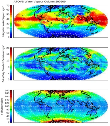
An example of ATOVS derived global monthly mean integrated water vapour content and corresponding extra daily standard deviation is shown in Fig.3. Global fields are provided in sinusoidal projection at a horizontal resolution of (90km)2. The daily and monthly mean products are merged products derived from all available ATOVS sensors 20

from NOAA 15, NOAA 16 and NOAA 18 platforms. The ATOVS system on MetOp will be added during 2008.

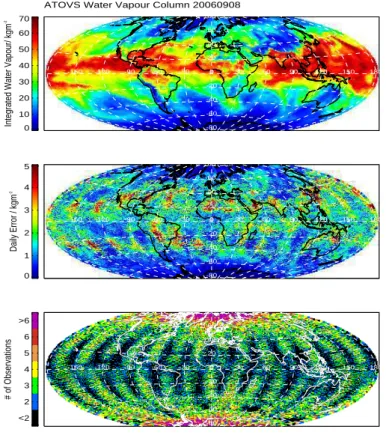
An optimal interpolation method (Kriging) is applied that provides a spatial distribu-tion of mean values and their errors. Fig.4 shows the daily mean, its corresponding error and the number of independent measurements per day for 8 September 2006. 25

The number of independent measurements from satellites is rather given by the num-ber of satellite overpasses because individual pixels cannot be treated as independent measurements (Lindau and Schulz,2004). The field shows the typical sampling with polar orbiters during one day with data gaps in the subtropical regions. Those gaps

(19)

ACPD

Full Screen / Esc

are effectively interpolated in the daily mean field. The corresponding error field for this day represents larger errors where no measurements are available and where the intra-daily variability is not well represented with 4–6 satellite overpasses per day as over the Gulf Stream region east of the USA. Large errors appear also in places where it is expected that the retrieval is hindered by difficult surfaces as over the Sahara where 5

knowledge of emissivity and the diurnal cycle of the surface temperature limit the qual-ity of the retrieval. As the method is also capable of handling retrieval errors and error covariances an improved error budget calculation is under development and will further enhance the quality of the error map.

SSM/I product

10

A total column water vapour estimate over ice free oceans is derived from measure-ments of the SSM/I employing the retrieval bySchl ¨ussel and Emery(1990). The above mentioned Kriging method is also used to combine the SSM/I measurements in an op-timal way. The record covers the period 1987–2005 and is updated in yearly intervals. This data set can be regarded as a climate data set suitable for long term variability 15

studies as all SSM/I radiometers have been intercalibrated using a statistical method described inAndersson et al.(2007).

3.2.2 Validation

ATOVS product

An initial validation of ATOVS results was performed for the period January 2004 to 20

December 2005 employing radiosonde data recorded at 173 Global Climate Observing System Upper-Air Network (GUAN) stations. The radiosonde data are used to validate the ATOVS daily averages on the (90km)2 grid. For this purpose the radiosonde data are allocated to the grid boxes and averaged over the day if more than one radiosonde ascent is available in a grid box. Note that a comparison to radiosonde data is more or 25

(20)

ACPD

Full Screen / Esc

less equivalent to a comparison of the product performance over land surfaces. Over ocean better results are expected because also the microwave instruments contribute to the product whereas over land it is mainly a HIRS product supported by the first guess of the retrieval. Additionally, the comparison is also slightly biased to the north-ern hemisphere as 56% of the GUAN stations are located there. On the southnorth-ern 5

hemisphere about 10% of the stations are located near the coast of Antarctica, which is a very difficult environment for the satellite product.

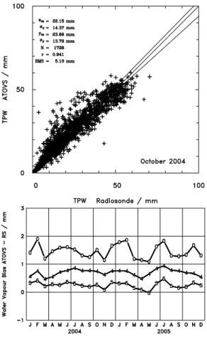
As an example Fig. 5shows a scatter plot for October 2004 indicating a very high correlation (0.94) between both data sets. Also visible is a positive bias of ∼1.5 mm in the ATOVS product. The lower part of Fig.5 shows the temporal development of this 10

bias for the whole period. The bias is varying between ∼1 mm and ∼2 mm with time. There is a slight tendency of higher biases in the northern hemisphere winter months that might be caused by less cloud free measurements over land. Fig.5 also shows that the bias is higher in the layer 850–700 hPa when compared to 1000–850 hPa. The GME model input used as background and first guess constrains the retrieval results 15

more strongly in the lowest atmosphere. This leads to a better agreement with the radiosondes in the lowest layer compared to the second lowest layer.

For the upper tropospheric layers (not shown)the relative bias is much lower, ∼2% for the 700–500 hPa layer and ∼1% for the 500–300 hPa layer, respectively. The results for the uppermost layer are difficult to interpret as integrated water vapour estimates 20

are already very small so that small absolute errors result in huge relative errors. How-ever, as the bias is positive one may say that this is consistent with the dry bias that radiosondes tend to have at this height.

SSM/I product

Schl ¨ussel and Emery(1990) did initial comparisons of instantaneous SSM/I total

col-25

umn water vapour retrievals to globally distributed radiosondes for data during July 1987. As collocation criteria they used matches within ±3 h and 0.5◦ latitude and lon-gitude. The sample size was around 300 matches and the bias and rms errors are 0.3

(21)

ACPD

Full Screen / Esc

and 5.6 mm, respectively. This result was confirmed by (Schulz et al.,1993) who found 0.4 mm for the bias and 5.8 mm for the rms using also data from August 1987.

The most recent and comprehensive analysis of total column water vapour content retrievals from passive microwave imagers has been done by (Sohn and Smith,2003). They compared five statistical (including theSchl ¨ussel and Emery (1990) algorithm) 5

and two physical algorithms in the framework of monthly and zonally averaged values. The global database of radiosondes used covered the period July 1987 to December 1990 (42 months). Statistics were derived from point pairings matched within 6 hours and 60 km. Most of the differences in bias and rms errors between the algorithms can be explained by different training data sets and different methods to exclude pixels with 10

high liquid water paths or rain. Considering regional differences between algorithms by comparing global monthly mean mapsSohn and Smith(2003) found that theSchl ¨ussel

and Emery (1990) is closest to theWentz(1995) optimum statistical algorithm, which had the best all around rms statistics. Maximum differences between these algorithms are 1.5 mm with well balanced positive–negative bias distribution.

15

Looking at zonally averaged water vapour contents (Fig. 12 inSohn and Smith,2003) it is striking that minimum and maximum excursions of the algorithms occur at equa-torial, subtropical, and mid-latitude latitudes, not unlike the zonally averaged profiles of cloudiness and precipitation. Sohn and Smith (2003) used the original brightness temperature thresholds of the published algorithms to exclude precipitating pixels from 20

the record. In the current software version used with CM-SAF this is not used. Instead, precipitation and cloud liquid water path retrieved from SSM/I data are used to sort out pixels. From this one may expect that minimum and maximum excursion are smaller with the new version.

The evaluation of the SSM/I retrieval schemes inSohn and Smith(2003) has shown 25

that the current CM-SAF scheme is fully competitive compared to other existing re-trievals. The presented comparison results from Sohn and Smith (2003) are based on SSM/I data from the DMSP F8 and F10 platforms that need substantial corrections be-cause of a non-functioning 85 GHz channel on F8 and large height and therefore zenith

(22)

ACPD

Full Screen / Esc

angle variations of the F10 satellite. It is not described if those features are corrected in the data used in the Sohn and Smith study. Thus the there found bias errors can be caused by a missing correction for those effects. However, the comparison statistics also show that the SSM/I is clearly the best suitable instrument for climate monitoring of vertically integrated water vapour over oceans.

5

3.3 Top of atmosphere radiation fluxes

Top of the atmosphere radiation fluxes can principally be used for the evaluation of the radiative budget of climate models and reanalysis. The temporal resolution of the geo-stationary satellite data (15 min) matches reasonably well with the time step of current global models and processes like convection and surface heating may be studied on a 10

time step basis. 3.3.1 Retrieval

The individual single satellite products from GERB and CERES on-board the AQUA and TERRA satellites are derived from the basic radiance measurements of the instru-ments. The CM-SAF top of atmosphere radiative flux products are merged from the 15

individual satellite products of GERB and CERES (seeHarries et al.(2005) for details). In that sense these products are level 3 products. The incoming solar radiative flux is determined from the Differential Absolute Radiometer DIARAD on-board the SOlar and Heliospheric Observatory (SOHO) satellite (Dewitte et al.,2004).

CM-SAF top of atmosphere radiative fluxes are available with high temporal and spa-20

tial resolution covering the full Meteosat disc and polar latitudes. On the Meteosat disc GERB measurements are used to benefit from its high temporal resolution. CERES measurements are exclusively used over polar regions with improved temporal sam-pling where GERB measurements are not available. GERB results are compared with CERES data in the solar spectral range to verify if measurements suffer from system-25

(23)

ACPD

Full Screen / Esc

the CERES instrument on the Tropical Rainfall Measurement Mission (TRMM) satellite using the Visible and InfraRed Scanner (VIRS) imager for scene identification (Loeb

et al.,2003), the longwave model stems from theoretical considerations based on ra-diative transfer calculations (Clerbaux et al.,2003).

Example products are shown in Fig.6 where the monthly mean top of atmosphere 5

thermal emitted flux and the solar reflected flux are given for June 2007. 3.3.2 Validation

The accuracy of the incoming solar flux product is dominated by the accuracy of the total solar irradiance, which is also referred to as “Solar Constant”. Recent studies have shown that the accuracy of the latter is about 1 W/m2(Crommelynck et al.,1995), 10

(Dewitte et al.,2001), thus being also the accuracy of the incoming solar flux product.

Validation of the thermal emitted flux and the reflected solar flux was carried out over different surface types. It is based on a comparison of results against Meteosat-7 retrieval results and an intercomparison of GERB and CERES radiance data. We found differences between the results of GERB and the three active CERES instruments of 15

about 3% (thermal emitted flux) and 6% (solar reflected flux), respectively, which is sufficient to fulfil current user requirements. We further analyzed unfiltered GERB and CERES radiance data and acceptable agreement (within postulated error margins) was found over homogeneous scene types, e.g. cloudy scenes (1–2%) and desert regions (4–6%), although GERB radiances are always higher. A systematic deviation of about 20

8% was found over clear sky ocean scenes which may partly be caused by the GERB spectral response function in use. Further work is under way to confirm this possible explanation.

3.4 Surface radiation fluxes

Incoming and outgoing solar and thermal radiative fluxes are also computed at ground 25

(24)

ACPD

Full Screen / Esc

pressure and cloud type as input. 3.4.1 Incoming solar radiation

The calculation of the surface incoming solar radiation (SIS) is based on the method of

(Pinker and Laszlo,1992) and (Mueller et al.,2004). It uses the well-known

relation-ship between the broadband atmospheric transmittance and the reflectance at the top 5

of atmosphere retrieved from GERB data by RMIB. The reflectance at the top of at-mosphere is affected by the atmospheric (e.g., clouds and aerosol) and surface (e.g., albedo) state. The relation between the solar irradiance and the top of atmosphere albedo is pre-calculated and saved in look-up tables for a manyfold of atmospheric states and surface albedos. These look-up tables are finally used to derive the solar 10

irradiance from the TOA albedo for a given surface albedo and atmospheric state by interpolation.

3.4.2 Downwelling longwave radiation

For the surface downwelling longwave radiation we adapted the algorithm developed

by (Gupta,1989), (Gupta et al.,1992). The parametrization requires the temperature

15

profile of the lowest layers of the atmosphere, the water vapour profile and the cloud base height. All atmospheric data used in the surface flux retrieval as well as for the surface albedo calculations are taken from Numerical Weather Prediction (NWP) mod-els. Here, the CM-SAF operational processing employs analysis data of the General Circulation Model (GCM) of the German Meteorological Service (DWD) with a spatial 20

resolution of about 40 km, a temporal resolution of three hours and 40 atmospheric layers up to 10 hPa (Majewski et al.,2002). The outgoing longwave flux at surface level is obtained from the Stefan-Boltzmann equation and a surface emissivity that depends on the surface type (Wilber et al.,1999). The surface temperature is again taken from NWP analysis data.

(25)

ACPD

Full Screen / Esc

3.4.3 Surface albedo

The broadband surface albedo at cloud free pixels is derived as follows: Firstly, the angular-dependent surface reflectance from the top of atmosphere reflectance (per channel) is computed by removing the atmospheric signal caused by gaseous absorp-tion, molecular and aerosol scattering. For this the forward model SMAC (Rahman and

5

Dedieu,1994) has been used for the required radiative transfer simulations. Viewing and illumination conditions are corrected employing bidirectional reflectance distribu-tion funcdistribu-tions for different surface types. The surface albedo is then calculated from surface reflectance data as suggested byRoujean et al.(1992). The broadband sur-face albedo is estimated from a narrow- to broadband conversion (Liang,2000). The 10

instantaneous surface albedo is finally computed by normalization to a solar zenith angle of 60◦.

3.4.4 Averaging procedure

Climatological studies require daily averages of the radiation fluxes. For the polar or-biter products the daily averages of the longwave flux are derived by linearly averaging 15

all available, but at least three NOAA overpasses during the day. The daily mean value of SIS is derived following the method presented in Diekmann et al. (1988), which takes into account the diurnal variation of the solar incoming clear-sky flux. Again, three overpasses per day must be at least available. Monthly averages require again at least twenty daily mean products. A daily mean is not feasible for surface albedo 20

as usually the clear sky area is rather small compared to the cloudy area. Instead, a weekly and monthly mean albedo is calculated from the instantaneous estimates. 3.4.5 Product examples

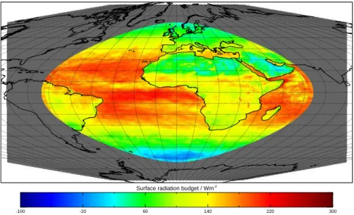
As an example and to demonstrate the need for high-resolution climatological data we show the incoming solar radiation based on SEVIRI data at surface level both on 25

(26)

ACPD

Full Screen / Esc

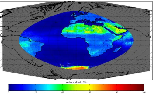
the spatial grids of the CM-SAF product and the National Centers for Environmental Prediction (NCEP) reanalysis (Fig. 7). Clearly, the much higher spatial resolution of CM-SAF is beneficial for many applications, not only for climate issues but also for e.g., the solar energy community, which is interested in radiation maps of European areas. Two other product examples, monthly mean results of September 2007 of the surface 5

albedo and the surface radiation budget based on METEOSAT-9/SEVIRI observations are shown in Figs.8and9, respectively.

3.4.6 Validation

The radiation products are validated against ground-based measurements, whereby mainly Baseline Surface Radiation Network (BSRN) stations are used (Ohmura et al., 10

1998), supplemented by specific well maintained measurements from European na-tional weather services. Validation of the instantaneous satellite derived data vs. hourly averaged surface measurements of the longwave components and the solar incom-ing irradiance showed good agreement within the targeted accuracy of 10 W/m2 for monthly averages. Larger deviations of the thermal radiation and the solar incoming 15

radiation are however found over complex terrain where ground-based measurements are not necessarily representative for larger areas of the size of satellite pixels (

Holl-mann et al.,2006).

It is essential to carefully consider the location of the station (height above sea level, horizontal view restrictions, multiple reflection effects, shadow effects) relative to the 20

surrounding area. Furthermore, local meteorological conditions of e.g., measurement sites in valleys may considerably hamper the interpretation of validation results. On the other hand, the spatial resolution of SEVIRI-based products cannot properly resolve the small-scale spatial variability of mountainous terrain. It seems further that the sep-aration of clouds and snow-covered scenes suffers from the low spatial resolution of 25

the standard solar SEVIRI channels. Thus, it is considered to introduce an improved SIS product that is based on high-resolution visible (HRV) channel of SEVIRI and a dig-ital elevation model to take into account topographic effects (D ¨urr and Zelenka,2007).

(27)

ACPD

Full Screen / Esc

As can be seen in Fig.10the calculated incoming solar radiation based on HRV data differs remarkably from the standard product. Validation of the solar incoming radiation against ground-based measurements taken from the Alpine Surface Radiation Bud-get network (ASRB) clearly shows the beneficial impact of the high-resolution channel (Fig.11). The scatter of SIS results is reduced and the negative bias of the SIS stan-5

dard product disappears if HRV data is used.

The relative accuracy of the surface albedo is approximately 25% with respect to ground-based measurements. This is the expected accuracy from the used space born sensors. However surface albedo retrieved from the geostationary SEVIRI instrument and the AVHRRR instrument systematically differ in their mean value. The reason for 10

this bias is not fully understood and currently under investigation.

4 Summary and future perspectives

CM-SAF as part of EUMETSAT’s SAF network provides satellite-derived thematic cli-mate data records. The CM-SAF products comprise macrophysical and cloud physical variables as among others cloud cover and cloud optical thickness, vertically resolved 15

temperature and water vapour information as well as resulting radiation fluxes at the top of the atmosphere and the surface. Spatial coverage of the products ranges from re-gional (AVHRR derived cloud parameters) over continental (SEVIRI full disc products) to global (ATOVS and SSM/I water vapour products). Temporal coverage is rather short for most of the CM-SAF data products because the operational production started in 20

2005 and no processing of historical data was foreseen. The exception to this is the SSM/I water vapour series that covers a period from 1987–2005.

CM-SAF utilizes most up to date retrieval schemes to derive its products from oper-ational satellite sensors. Validation results as described above revealed encouraging results for all products, although particular problems such as the systematic difference 25

between surface albedo derived from AVHRR and SEVIRI remain to be solved. Cur-rently available products can already be used for several applications including

(28)

vari-ACPD

Full Screen / Esc

ability analysis at diurnal to subseasonal time scales, improvements of cloud parame-terizations in climate models, etc. Series based on already intercalibrated data as the CERES referenced top of atmosphere radiation fluxes and the intersensor calibrated SSM/I water vapour data can also be used for studies of inter-annual variability. Solar radiation fluxes at the surface are also beneficial for the solar energy community. 5

Based on recommendations from GCOS, the WMO Space Programm, and EUMET-SAT, CM-SAF has identified four key issues for the future development of the CM-SAF data sets in a time frame of 5–10 years. These are:

1. Calibration

Requirements for more accurate satellite information products are steadily in-10

creasing. To create the stable long-term data sets needed for monitoring cli-mate change it becomes vital to inter-calibrate sensors on similar and different satellites. To integrate observations and products from different satellite systems, the measurements must be inter-calibrated. For instanceRoebeling et al.(2006) investigated the differences between cloud properties derived from SEVIRI on 15

Meteosat 8 and AVHRR on the NOAA-17 platform. It clearly showed the need of intercalibration before integration. Otherwise the data cannot be used for cli-mate applications because jumps (systematic biases) can occur in a time series constructed from different sensor observations.

Relative calibration of satellite data is a pre-requisite for a reasonable processing 20

of data obtained from different sensors of the same type. Current schedule of MSG launches shows that data from three spacecrafts will need to be harmonised until 2012. It is however expected that the satellite operator (EUMETSAT) will provide such radiance data sets towards the end of the CDOP.

First attempts to generate sensor intercalibrated brightness temperature time se-25

ries from SSM/I records have already been undertaken in the framework of the HOAPS-3 data set (Andersson et al.,2007). Those basic data have already been used to build the SSM/I water vapour product. Furthermore, it is envisaged to

(29)

ACPD

Full Screen / Esc

retrieve global cloud products using the satellite intercalibration that was devel-oped to generate the PATMOS-X data set (Jacobowitz et al.,2003), but replacing the retrieval methods with CM-SAF cloud algorithms. Such complementary time series would be quite helpful to identify algorithm weaknesses and strengths. International activities like the Global Space-based Inter-Calibration System 5

(GSICS) initiative strongly help to fulfil some of the CM-SAF needs with respect to data sets and methods during the CDOP. However, some intercalibration ac-tivities may have to be pursued by CM-SAF especially in those cases where non EUMETSAT sensors like the SSM/I are used or newer instruments like SEVIRI must be homogenised with older instruments like MVIRI on the Meteosat first 10

generation in due time. The global network of Regional Specialized Satellite Cen-ters on Climate Monitoring (R/SSC-CM) planned by WMO will help to foster the international collaboration in the generation of intercalibrated radiance records. The R/SSC-CM will also help to organize the production and quality assessment of geophysical data sets derived from the intercalibrated radiance records. 15

2. Temporal extension of the data sets and reprocessing of current products based

on intercalibrated sensor data and employing improved and frozen retrieval schemes

Climate change and variation occur on different time scales and data sets use-ful for climate monitoring must therefore cover longer time series to understand 20

these changes. The demands on the accuracy increase in accordance to the time scales considered. Today the existing CM-SAF data sets are suitable for monitor-ing diurnal and subseasonal to seasonal fluctuations of environmental variables, which can be large.

At the seasonal to interannual time scale the accuracy requirements increase 25

dramatically because climate phenomena at this scale are initiated by very small changes in the observed parameters. At decennial to centennial time scales, which are exclusively suitable for trend detection, the accuracy of data sets must

(30)

ACPD

Full Screen / Esc

be one order of magnitude higher than compared to the needs of detecting in-terannual fluctuations. Thus, CM-SAF will also process historical satellite data to ensure that its data sets may become suitable for trend detection. Further-more, improvements of retrieval algorithms and the growing time series of newer instruments such as SEVIRI that are affected by calibration changes will cause 5

reprocessing of these data sets within the period 2007 to 2012. Both activities im-ply close interaction of responsible space agencies in order to archive and provide the required data in the given time frame. Such reprocessing events also need to be carefully coordinated with data suppliers (upstream) and the user community (downstream).

10

3. The production of global and regional products

Climate variability at regional level may be related to global climate changes but regional effects may differ from region to region. CM-SAF aims to provide support for climate analysis at regional level but needs global products to improve the un-derstanding of scale interaction and to interpret the nature of regional changes. 15

Global products enhance the amount of possible applications, e.g., global prod-ucts can be used to support studies on climate sensitivity of global climate models. However, the extension to global products is not possible for all products because of the inhomogeneity of the observing system. This is especially true for instru-ments in geostationary orbit where the SEVIRI instrument sets new standards 20

but dedicated algorithms cannot be applied globally. Additionally, collaboration between at least four satellite operators would be needed to achieve an almost global product. Regional products derived from SEVIRI with improved quality will still serve as regional benchmark data sets. Products from polar orbiters typically suffer from inadequate spatiotemporal sampling at low latitudes but provide com-25

plementary data with often better spatial resolution. However, at high latitudes polar orbiter data are essential to study polar conditions.

(31)

ACPD

Full Screen / Esc

and water cycle

The primary strength of the CM-SAF approach for climate monitoring is the pro-vision of consistent thematic climate data records. One of the most concerning questions about the changing Earth climate system is the potential change of the hydrological and energy cycle. Energy and water cycle related geophysical pa-5

rameters over water surfaces at global scale are provided by the Hamburg Ocean Atmosphere Parameters and Fluxes from Satellite Data (HOAPS-3) (Andersson

et al.,2007). Consequently, CM-SAF will take over the responsibility for the pro-cessing of HOAPS during the CDOP. This will enhance the product suite with precipitation and turbulent heat fluxes over the ocean. Potentially, the CM-SAF 10

surface flux products can be used to investigate the net heat flux at the ocean surface.

A 30 year long climatology of upper tropospheric humidity derived from a homog-enized Meteosat record spanning over Meteosat First and Second Generation instruments will be derived in cooperation with the Laboratoire M ´et ´eorologie Dy-15

namique (LMD). It will provide a very good data set to study the variability of water vapour at intra-seasonal scale. Brogniez et al.(2006) found from a series of Me-teosat First Generation data for the period 1983–2005 an asymmetry between the two hemispheres along the annual cycle. Whereas the intra-seasonal variability is homogeneous in the Southern hemisphere the variability shows a distinct min-20

imum in the Northern hemisphere during the summer. Thus, the planned data set extended with data from the new SEVIRI instrument will be perfectly usable to analyse the quality of intra-seasonal variability in future global reanalysis. Other new products include ice water path, aerosol properties and enhanced surface radiation flux products as a spectrally resolved irradiance.

25

Acknowledgements. We acknowledge the Cloudnet project (European Union contract

EVK2-2000-00611) for providing the microwave radiometer and target classification data, which was produced by the University of Reading using measurements from the experimental sites of Chilbolton in the UK, Paleaseau in France and Cabauw in the Netherlands. The supportive work