HAL Id: hal-00305158
https://hal.archives-ouvertes.fr/hal-00305158
Submitted on 19 Mar 2008
HAL is a multi-disciplinary open access
archive for the deposit and dissemination of
sci-entific research documents, whether they are
pub-lished or not. The documents may come from
teaching and research institutions in France or
abroad, or from public or private research centers.
L’archive ouverte pluridisciplinaire HAL, est
destinée au dépôt et à la diffusion de documents
scientifiques de niveau recherche, publiés ou non,
émanant des établissements d’enseignement et de
recherche français ou étrangers, des laboratoires
publics ou privés.
using ensemble learning
J. Peters, B. de Baets, R. Samson, N. E. C. Verhoest
To cite this version:
J. Peters, B. de Baets, R. Samson, N. E. C. Verhoest. Modelling groundwater-dependent
vegeta-tion patterns using ensemble learning. Hydrology and Earth System Sciences Discussions, European
Geosciences Union, 2008, 12 (2), pp.603-613. �hal-00305158�
www.hydrol-earth-syst-sci.net/12/603/2008/ © Author(s) 2008. This work is distributed under the Creative Commons Attribution 3.0 License.
Earth System
Sciences
Modelling groundwater-dependent vegetation patterns using
ensemble learning
J. Peters1, B. De Baets2, R. Samson3, and N. E. C. Verhoest1
1Department of Forest and Water Management, Ghent University, Coupure links 653, 9000 Gent, Belgium 2Department of Applied Mathematics, Biometrics and Process Control, Coupure links 653, 9000 Gent, Belgium 3Department of Bioscience Engineering, University of Antwerp, Groenenborgerlaan 171, 2020 Antwerpen, Belgium
Received: 17 September 2007 – Published in Hydrol. Earth Syst. Sci. Discuss.: 2 October 2007 Revised: 12 February 2008 – Accepted: 14 February 2008 – Published: 19 March 2008
Abstract. Vegetation patterns arise from the interplay
be-tween intraspecific and interspecific biotic interactions and from different abiotic constraints and interacting driving forces and distributions. In this study, we constructed an ensemble learning model that, based on spatially distributed environmental variables, could model vegetation patterns at the local scale. The study site was an alluvial floodplain with marked hydrologic gradients on which different vegetation types developed. The model was evaluated on accuracy, and could be concluded to perform well. However, model ac-curacy was remarkably lower for boundary areas between two distinct vegetation types. Subsequent application of the model on a spatially independent data set showed a poor per-formance that could be linked with the niche concept to con-clude that an empirical distribution model, which has been constructed on local observations, is incapable to be applied beyond these boundaries.
1 Introduction
Ecosystems are complex, evolving structures whose charac-teristics and dynamic properties depend on many interrelated links between direct gradients (nutrients, moisture, temper-ature), their environmental determinants (climate, geology, topography) and potential natural vegetation, and the pro-cesses that mediate between the potential and actual vege-tation cover (Baird and Wilby, 1999). Riparian wetlands in
Correspondence to: J. Peters
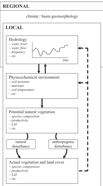
particular exhibit a complex interplay between meteorolog-ical, hydrological and biological processes and interactions with the surrounding terrestrial and aquatic systems result-ing in a high spatial and short-term variability (Dall’O’ et al., 2001). The conceptual representation shown in Fig. 1 illustrates the relationships between hydrology, the physic-ochemical environment and vegetation at the local scale. The direct effect of site hydrology on physicochemical site properties, such as soil moisture content, oxygen and nutri-ent availability determines the productivity and species com-position of the site (Venterink et al., 2001; Wassen et al., 2003). Vegetation, however, is not passive to the abiotical setting, but affects site hydrology and physicochemical prop-erties through feedback processes of which transpiration (En-gel et al., 2005), soil aeration (Mainiero and Kazda, 2005) and alterations in nutrient loadings (Hill, 1996; Fisher and Acreman, 2004) are just some examples. These localized direct and feedback processes result in spatial and tempo-ral distributions of the abiotical constraints at a higher scale level (Schr¨oder, 2006). Together with intraspecific, interspe-cific and anthropogenic interactions these distributed abioti-cal constraints result in vegetation patterns.
Exploring vegetation patterns is a central goal in ecol-ogy. Numerous studies examined environmental gradients in relation to vegetation type distributions in various ecosys-tems (Schulze et al., 1996; Famiglietti et al., 1998; Molina et al., 2004; Rudner, 2005), and different techniques have been developed to quantify vegetation-environment relationships. Canonical ordination (Jongman et al., 1995) for example, is widely applied in ecological studies to detect patterns of vari-ation in vegetvari-ation data and quantify the main relvari-ations be-tween vegetation and environmental variables. Generalized
REGIONAL
climate / basin geomorphology
LOCAL
Potential natural vegetation
~ species composition ~ productivity ~ LAI ~ etc. Physicochemical environment ~ soil moisture ~ nutrients ~ soil temperature ~ etc. Hydrology ~ water level ~ water flow ~ frequency ~ etc. time
Actual vegetation and land cover
~ species composition ~ productivity ~ LAI ~ etc. natural disturbance anthropogenic disturbance
Fig. 1. Conceptual model illustrating the relationships between
hy-drology, the physicochemical environment and vegetation at the lo-cal slo-cale. Legend: full arrows indicate direct effects, broken arrows indicate vegetation feedbacks, and rounded squares and bent arrows indicate exogenous disturbances. Figure adapted from Franklin (1995); Baird and Wilby (1999); Mitsch and Gosselink (2000).
linear models (e.g. multiple logistic regression (Hosmer and Lemeshow, 2000)) are frequently applied to construct distri-bution models (Austin, 2002; Bio et al., 2002, among oth-ers). Distribution models tend to predict spatial distribu-tions of species based on environmental variables (Guisan and Zimmerman, 2000; Guisan and Thuiller, 2005). In this study, an ensemble learning technique named random forests (Breiman, 2001; Prasad et al., 2006), is applied to a spatially distributed data set containing information on environmen-tal conditions and vegetation type distributions. The random forest distribution model was assessed in terms of: (i) its
clas-Observations LEGEND A B C D E
Fig. 2. The Doode Bemde is situated in the valley of the river Dijle.
A detailed overview of the topography and the vegetation distribu-tion at the site are shown. The posidistribu-tions of 5 (A-E) piezometers located along a topographical transect are symbolized by ◦.
sification accuracy, (ii) its applicability on a similar alluvial floodplain, and (iii) its potential to model vegetation distribu-tions based on a reduced number of important environmental variables in groundwater-dependent ecosystems.
2 Description of the study site
A lowland river valley in Belgium called “Doode Bemde” was the research area of this study (Fig. 2). The site is an alluvial floodplain mire in the middle course of the river Di-jle, situated approximately 30 m above sea level. The area is bordered by the river Dijle in the west, the Molenbeek, a tributary of the Dijle, in the north and the valley slope with a number of permanent springs in the east (De Becker et al., 1999). The climatic conditions at the site are typically temperate, with an average yearly rainfall of ≈800 mm dis-tributed evenly over the year (Verhoest et al., 1997; De Jongh et al., 2006), an average annual pan evaporation of 450 mm, and an average yearly air temperature of 9.8◦C (Van Herpe and Troch, 2000). Local conditions at the Doode Bemde have been extensively described by De Becker et al. (1999) and Joris and Feyen (2003).
2.1 Ecohydrological monitoring scheme
During the summer of 1993 and the spring of 1994, plant species occurrences were mapped in the study area. There-fore, the total area of 21.08 ha was subdivided in 519 regular and adjacent 20 m by 20 m grid cells. Mapping was restricted to a selection of 56 plant species of which 45 were typically groundwater dependent (phreatophytes, sensu Londo (1988)) and 11 were differential species for several vegetation types at the Doode Bemde. Based on these species cover data, De Becker et al. (1999) applied TWINSPAN (Hill, 1979) in or-der to define vegetation types. Seven different types were
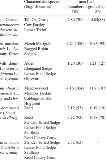
Table 1. Summary of the vegetation types: abbreviation, name, short description and area.
Nr. Name Short description Characteristic species area [ha]
(English names) (number of grid cells)
DB SN
Ar Arrhenatherion High yield potential pasture.
Charac-teristic species include Arrhenatherum elatius (L.) J. & C. Presl, Anthriscus sil-vestris (L.) Hoffm. and Trifolium du-bium Sibth..
Tall Oat Grass Cow Parsley Lesser Trefoil
2.80 (70) 0.83(83)
Cp Calthion palustris Species–rich mesotrophic fen meadow
dominated by Caltha palustris L., Ly-chnis flos–cuculi L., and many Carex species. March Marigold Ragged Robin Sedges 4.24 (106) 0.93 (93) Ce Carici elongetae – Alnetum glutinosae
Mesotrophic forest type with domi-nance of Alnus glutinosa (L.) Gaertn. and a herblayer with Carex elongata L., Carex acutiformis Ehrh. and Lycopus europaeus L..
Alder
Elongated Sedge Lesser Pond Sedge Gipswort
1.20 (30) 1.21 (121)
Fi Filipendulion Tall herb fen with Filipendula ulmaria
(L.) Maxim., Alopecurus pratensis L., Cirsium oleraceum (L.) Scop. and Her-acleum sphondylium L.. Meadowsweet Meadow Foxtail Cabbage Thistle Hogweed 4.16 (104) 1.07 (107)
Ph Phragmitetalia Highly fertile reedswamps dominated
by Phragmites australis (Cav.) Steud..
Reed 2.12 (53) 0.19 (19)
MP Magnocaricion with
Phragmites
Magnocaricion vegetation with Phrag-mites australis (Cav.) Steud..
Reed
Slender Tufted Sedge Lesser Pond Sedge Skullcap
Reed Canary Grass
3.72 (93) 0.78 (78)
Ma Magnocaricion Tall sedge swamp with Carex acuta
L., Carex acutiformis Ehrh., Scuttelaria galericulata L. and Phalaris arundi-nacea L..
Slender Tufted Sedge Lesser Pond Sedge Skullcap
Reed Canary Grass
2.52 (63) –
DB = Doode Bemde; SN = Snoekengracht
distinguished (Table 1), and their spatial distribution can be seen in Fig. 2. All vegetation types are herbaceous, except for Carici elongetae – Alnetum glutinosae where a tree layer of Common Alder is present. The similarity in species com-position between grid cells was compared using the Jaccard index of similarity JS=c/(a+b+c) where c is the number of species shared by both cells, and a and b are the numbers of species unique to each of the cells (Jaccard, 1912). The Jaccard similarity of two grid cells expresses their ecological resemblance concerning species composition, and ranges be-tween 0 (when both cells have unique species) and 1 (when both cells have equal species composition). Averaged JS values are given in Table 2 for the seven different vegeta-tion types. The values of the diagonal elements in Table 2 are a measure of similarity between grid cells of the same vegetation type. Based on these values, patches of
Phrag-mitetalia, Magnocaricion with Phragmites and Magnocari-cion can be concluded to be more homogeneous in species
composition compared to the other vegetation types which have lower values. Between the different vegetation types, marked differences in similarity can be observed.
Magno-caricion with Phragmites has high similarities with Phrag-mitetalia and Magnocaricion. Between the other vegetation
types, similarities are generally lower, but nevertheless dif-ferences can be observed. Arrhenatherion for example, has twice as much species in common with Filipendulion than with Magnocaricion.
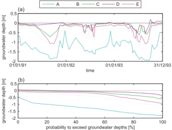
A groundwater monitoring network consisting of 25 piezometers was installed in 1989. Groundwater depths were measured every fortnight during the period 1 January 1991–31 December 1993. Time series of linear interpolated groundwater depths measured at several piezometers (A–E, locations can be seen in Fig. 2) along a topographical transect are plotted in Fig. 3a. A yearly pattern of high summer depths and low winter depths was observed at all piezometers. Based on these time series, hydrological dura-tion lines expressing the probability (%) that a groundwater
Table 2. Jaccard index of similarity between the vegetation types in
the Doode Bemde.
Ar Cp Ce Fi Ph MP Ma Ar 0.40 Cp 0.18 0.37 Ce 0.11 0.17 0.46 Fi 0.24 0.21 0.20 0.39 Ph 0.09 0.19 0.35 0.22 0.55 MP 0.10 0.19 0.30 0.23 0.44 0.51 Ma 0.11 0.24 0.30 0.33 0.38 0.42 0.54
depth is exceeded are calculated (Fig. 3b). Groundwater depths corresponding to a probability of exceedance of 50% are yearly average groundwater depths. They differed con-siderably along the transect (Fig. 3b). At the levee near the river an average value of 1.27 m was measured (piezometer A), which decreased gradually moving further down toward the depression (piezometer B→C→D), with a minimal yearly average groundwater depth of 0.05 m measured at piezometer D in the center of the depression. Fig. 3b also shows different periods of superficial groundwater depths (<0.3 m) in all piezometers, ranging from 75% of the year in piezometer C to 35% of the year in piezometers B and D. Groundwater depths measured in piezometer A are never <0.3 m. Additional to the monitoring of groundwater dynamics, all 25 piezometers were sampled on several groundwater quality variables during a sampling campaign in September 1993 with respect to pH, Cl−, Ca2+, Fetot, K+,
Mg2+, NO−3-N, NH+4-N, H2PO−4 and SO2−4 . All values are
in [mg L−1] except for pH [-]. A soil type map was made based on 60 drillings to a depth of 1 m, evenly distributed over the study area. Management regime was assessed for each grid cell separately. Four different regimes could be distinguished:
– Yearly mowing in early summer, followed by grazing or
mowing of the aftermath;
– Cyclic mowing (once every 5 to 10 years) or not mown
at all since at least 5, and up to 10 years;
– No management for at least 10 years; – Transition from yearly to cyclic mowing.
2.2 Data set
Groundwater depth measurements were used to calculate a dynamic groundwater variable, the mean groundwater depth (MGD) below surface [m]. Values of this variable, together with the groundwater quality variables, were assigned to each grid cell by spatial interpolation of measurement data over the entire area using block kriging (for details, see Bio et al. (2002)). 01/01/91-2 01/01/92 01/01/93 31/12/93 -1.5 -1 -0.5 0 0.5 time groundwater depth [m] 0 20 40 60 80 100 -2 -1.5 -1 -0.5 0 0.5
probability to exceed groundwater depths [%]
groundwater depth [m] A B C D E (a) (b)
Fig. 3. (a) Time series of the groundwater depth, as monitored by
piezometers A–E along a topographic transect (see Fig. 2). (b) Hy-drological duration lines expressing the probability that measured groundwater depths are exceeded. The line colours correspond to the vegetation types wherein these piezometers were installed (see Fig. 2).
The spatially explicit variables were structured into a data set. The data set contains N =519 measurement vectors
xi=(xi1, xi2, . . . , xip) consisting of the values of p=13 vari-ables describing the abiotic environment:
– Groundwater dynamics: mean groundwater depth
(con-tinuous variable);
– Groundwater quality: pH, Cl−, Ca2+, Fetot, K+, Mg2+,
NO−3–N, NH+4–N, H2PO−4 and SO2−4 . All these
vari-ables are continuous;
– Soil: soil type (silt/peat, categorical);
– Management: yearly mowing, cyclic mowing, no
man-agement, transition (categorical).
Seven different vegetation types c1, . . . , c7 are considered.
To each measurement vector xia unique vegetation type li ∈
{c1, . . . , c7}is assigned. The data set will be denoted as:
L = {(x1, l1), . . . , (xN, lN)} . (1) 2.3 Independent evaluation data set
A spatially independent ecohydrological data set Lev was constructed for a similar valley ecosystem, “Snoekengracht”. The Snoekengracht is an alluvial floodplain of the river Velp, situated approximately 15 km from the Doode Bemde. The climatic setting of both nature reserves is very much alike, and local environmental conditions and floral composition are very similar (Bio et al., 2002). The monitoring scheme was largely the same as in the Doode Bemde (Huybrechts and De Becker, 1999), and a grid-based (with a grid size of
10 m by 10 m) data set consisting of M=501 elements was constructed, which will be denoted as:
Lev= {(y1, l1), . . . , (yM, lM)} . (2) where liis the vegetation type assigned to measurement vec-tor yi. Most vegetation types coincide with those found at Doode Bemde, except for Magnocaricion which was not found at Snoekengracht (see Table 1).
3 Distribution model
The distribution model used in this study applies the random forest technique (Breiman, 2001). Random forest is an en-semble learning technique which generates many classifica-tion trees (Breiman et al., 1984) that are aggregated to com-pute a classification. Each classification tree is grown using another bootstrap subset Liof the original data set L and the nodes are split using the best split variable among a subset of m randomly selected variables (Liaw and Wiener, 2002). The pseudo-code for growing a random forest is given in Ap-pendix A1. The number of trees (k) and the number of vari-ables used to split the nodes (m) are two user-defined param-eters required to grow a random forest. An unbiased estimate of the generalization error (the so called out-of-bag error, oob error) is obtained during the construction of a random forest (Appendix A2). Breiman (2001) proved that random forests produce a limiting value for the oob error. As the number of trees increases, the generalization error always converges. The number of trees (k) needs to be set sufficiently high to allow for this convergence. The oob error can be used to op-timize the other user-defined parameter m, in order to get a minimal random forest error (Peters et al., 2007). The model outcome is an ensemble of k classification trees which are aggregated based on majority votes to compute the final clas-sification. Since every classification tree votes for a certain vegetation type cj based on the measurement vector xi of grid cell i, the probability of occurrence of vegetation type
cj is given by P (cj) = Ncj/ k, where Ncj is the number of trees voting for vegetation type cj, and k the total number of trees. The highest probability of occurrence (P (cj)max)
determines the predicted vegetation type cj.
Additionally, the random forest algorithm can estimate variable importances (Appendix A3), i.e. variables can be ranked according to their importance in determining vege-tation distributions at the study site.
4 Modelling vegetation distributions
4.1 Model construction and results
At first instance the data set L was randomly split into 3 data subsets for 3-fold cross-validation. The model was constructed using the random forest program provided by Breiman and Cutler (2005). User-defined parameters m, the
Table 3. Confusion matrix of the classification made by the random
forest distribution model. Predicted vegetation types are compared with the observations at the Doode Bemde.
Observed Ar Cp Ce Fi Ph MP Ma Predicted Ar 55 4 0 4 0 0 0 Cp 6 89 0 7 0 5 4 Ce 0 1 19 0 1 4 4 Fi 9 2 0 82 1 0 7 Ph 0 2 7 1 45 4 2 MP 0 2 3 1 4 68 9 Ma 0 6 1 4 2 12 37
number of randomly selected variables to split the nodes, and
k, the number of trees within the random forest, where
op-timized using the oob error, and suitable parameter values were m=3 and k=1000. The results include an ensemble of
k=1000 predictions, one made by each classifier, which are
aggregated based on majority votes into a final classification. A confusion matrix summarizing the final classification is given in Table 3, and results are shown in Fig. 4a.
4.2 Model evaluation 4.2.1 Classification accuracy
Out of the 519 grid cells included in the study, the model classified 395 (76.1%) correctly, and 124 (23.9%) incorrectly (Table 3). A κ (Cohen, 1960) value of 0.716 was calculated, indicating a substantial agreement between observations and predictions. A threshold-independent evaluation using re-ceiver operating characteristic (ROC) graphs was performed (Hosmer and Lemeshow, 2000). ROC graphs are useful for visualizing classifier performances (Fawcett, 2006). ROC graphs are two-dimensional graphs in which the true posi-tive rate, tp, is plotted on the y-axis, and the false posiposi-tive rate, fp, on the x-axis, where
tp = positives correctly classified
total positives (3)
fp = negatives incorrectly classified
total negatives . (4)
The area under the ROC curve, abbreviated AUC, is a scalar value between 0 and 1 representing the classifier perfor-mance (Fawcett, 2006). Since random guessing produces a diagonal line between (0,0) and (1,1) in ROC space, with an AUC value of 0.5, a classifier with a higher AUC value than 0.5 does better than random guessing. For multi-class ROC graphs, which should be applied here since 7 vegetation types are considered, a methodology described in Fawcett (2006) is used. For each class a different ROC curve is produced, with ROC curve j plotting the classification performance using
Predictions Observations LEGEND (a) (a) (b) LEGEND (b) Probability class
Fig. 4. (a) Observed vegetation types overlaid by the classification
made by the random forest distribution model. (b) Modelled prob-abilities (P (cj)max) on which the classification is based.
vegetation class cj as positive and all other classes as neg-ative. For each ROC curve, the AUC can be calculated and averaged over the different classes using class weights based on class prevalences in the test data (Provost and Domingos, 2001):
AUCtotal =
X
cj∈C
AUC(cj) · w(cj) (5)
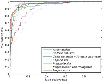
where AUC(cj) is the area under the class reference ROC curve for cj, and w(cj) a weighing factor. Weighing fac-tors are obtained from Table 1. Figure 5 visualizes the ROC curves for each vegetation type. The AUCtotal value equals
0.96 and the random forest distribution model is concluded to perform well. 0 0.2 0.4 0.6 0.8 1 0 0.1 0.2 0.3 0.4 0.5 0.6 0.7 0.8 0.9 1
false positive rate
true positive rate
Arrhenaterion Calthion palustris
Carici elongetae − Alnetum glutinosae Filipendulion
Phragmitetalia
Magnocaricion with Phragmites Magnocaricion
Fig. 5. Receiver operating characteristic (ROC) curves
visualiz-ing the classification performances of the 3-fold cross-validated random forest distribution model for the 7 vegetation types (full curves). The AUCtotalequals 0.96. Model performances for bound-ary cells only are summarized by the dashed ROC curves, yielding an AUCtotalvalue of 0.92.
4.2.2 Spatially explicit evaluation
For each grid cell, the ensemble of k=1000 classification re-sults is aggregated by calculating probabilities of occurrence
P (cj) for all j vegetation types of which the vegetation type with the highest P (cj) value (P (cj)max) is the predicted one.
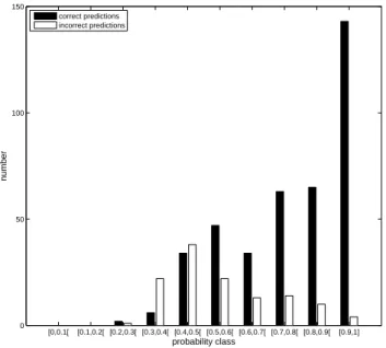
As seen in Fig. 6 this decision rule leads to an increasing number of correct classifications with increasing P (cj)max
values. Indeed, 252 elements are correctly classified with a probability higher than 0.7, whereas only 2 elements are cor-rectly classified with a probability lower than 0.3. 50% of the correctly classified elements are based on probabilities
>0.78. The incorrect classifications show a maximum in the
[0.4,0.5] interval, with 1 element incorrectly classified with a probability lower than 0.3, and 28 elements incorrectly clas-sified with probabilities higher than 0.7. 50% of the incor-rectly classified elements are based on probabilities > 0.55.
Figure 4b shows the spatial distribution of P (cj)max
val-ues at the study site in graduated colours. Correctly classi-fied grid cells with high P (cj)maxvalues are situated within
the central areas of homogeneous vegetation clusters, and
P (cj)max values tend to decrease toward the boundaries of
these areas (see also Fig. 4a). Incorrectly classified grid cell are mainly found where two adjacent vegetation types meet, and are based on low P (cj)maxvalues at the central
depres-sion and the north-eastern side of the study site. The vegeta-tion types found in these areas are Carici elongetae-Alnetum
glutinosae, Phragmitetalia, Magnocaricion with Phragmites
and Magnocaricion. A Jaccard similarity matrix was con-structed for the boundary grid cells only (Table 4). The JS
[0,0.1[ [0.1,0.2[ [0.2,0.3[ [0.3,0.4[ [0.4,0.5[ [0.5,0.6[ [0.6,0.7[ [0.7,0.8[ [0.8,0.9[ [0.9,1] 0 50 100 150 probability class number correct predictions incorrect predictions
Fig. 6. Probability distribution of correct and incorrect classified
grid cells of the Doode Bemde (N =519).
values in Table 4 express averaged resemblances in species composition of each boundary grid cell with its 8 neighbor-ing grid cells. Boundary grid cells of Phragmitetalia,
Mag-nocaricion with Phragmites and MagMag-nocaricion can be
con-cluded to share a large proportion of their species with JS values higher than 0.5. This is reflected in the modelling results, P (cj)max values for these grid cells are generally
low because comparable numbers of the k=1000 classifiers classify these grid cells as Phragmitetalia, Magnocaricion with Phragmites and Magnocaricion. Another conclusion should be drawn for isolated grid cells and small isolated vegetation clusters surrounded by another vegetation type (e.g. as occurs along the western border of the study area, see Fig. 4a). These grid cells are frequently incorrectly clas-sified with high P (cj)max values, and are the weak point
of the random forest distribution model. The worse perfor-mance of the model on boundary grid cells can also be seen in Fig. 5, where ROC curves of classification results computed for boundary grid cells only are lower than those computed for the entire data set. The corresponding AUCtotalvalue for
model performances in boundary areas equaled 0.92, while being 0.96 for the entire study area.
4.2.3 Performance on independent test data
The use of independent test data allows us to assess the model generalization abilities. Edwards et al. (2006) pointed out that cross-validated model accuracies are frequently differ-ent from accuracies assessed with truly independdiffer-ent data. It is easy to conclude that the random forest vegetation dis-tribution model, which was trained on the data set L did not classify data set Lev satisfactory. From the 501
ele-Table 4. Jaccard index of similarity for boundary grid cells between
two vegetation types at the Doode Bemde. Non-adjacent vegetation types are indicated by –.
Ar Cp Ce Fi Ph MP Ma Ar 0.59 Cp 0.38 0.60 Ce – 0.45 0.66 Fi 0.34 0.21 – 0.54 Ph – 0.18 0.52 0.27 0.67 MP – 0.30 0.36 0.19 0.57 0.65 Ma – 0.34 0.39 0.57 0.59 0.53 0.66 -5 -4 -3 -2 -1 0 1 2 3 4 -6 -4 -2 0 2 4 6 PCA 1 PCA 2
Calthion palustris at the Doode Bemde Calthion palustris at the Snoekengracht
Fundamental niche
Realized niche at Snoekengracht
Realized niche at Doode Bemde
Fig. 7. Conceptual representation of realised niches of Calthion
palustris at the Doode Beemde and Snoekengracht. The funda-mental niche of Calthion palustris ranges over all environfunda-mental states which would permit to Calthion palustris to exist indefinitely (Hutchinson, 1957).
ments included in Lev, only 99 elements were classified
cor-rectly (19.8%). This can be explained by the niche con-cept (Hutchinson, 1957). The fundamental niche of a plant species, and by extension a vegetation type, is defined as an
n-dimensional hypervolume (Hutchinson, 1957) in which
ev-ery point corresponds to a state of the environment which would permit the species to exist and reproduce. Due to interspecific competition species generally occupy only an elementary part of this volume, the realized niche. The niches realized by each of the vegetation types found at the Doode Bemde differ from those realised by the same vege-tation types at Snoekengracht. Although similar results were observed for all vegetation types, the example of Calthion
palustris is given in Fig. 7. Since 13 environmental
vari-ables are used in this study, a principle component analy-sis was performed to reduce dimensions and make results visible. Fig. 7 graphs the component scores of grid cells where Calthion palustris was observed on the 2 principle
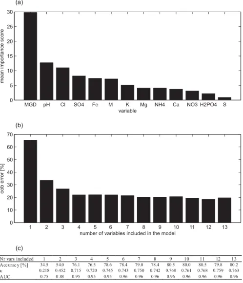
Fig. 8. (a) All variables ranked according to their importance as calculated with the variable importance measure (Appendix A3). M
stands for management regime, S represents the variable soil type, and MGD the mean groundwater depth. (b) Oob error of random forest distribution models constructed on data sets with reduced complexity. The model containing only the most important variable (MGD) has an oob error of 65.5%. The oob error decreases gradually when more variables are included. (c) Summarizing table of model performances: accuracy, Cohen’s κ and AUC values associated with a decreasing number of variables included.
component axes (cumulatively explaining 70% of variance). Although partly intersecting, two different realized niches can be distinguished. Obviously, a random forest distibution model that is trained on the vegetation distributions at the Doode Bemde and which uses explicit environmental thresh-olds to compute a classification, cannot perform well on such an independent test data set of an apparantely similar ecosys-tem.
5 Reduction of model complexity
The random forest algorithm includes a procedure to estimate the importance of the independent variables (Appendix A3).
Applying this procedure on data set L results in a ranking of all 13 variables according to importance (Fig. 8a). The most important variable is mean groundwater depth. This means that, according to this classification technique, the spatial dif-ferences in mean groundwater depths at the Doode Bemde are determinative for the vegetation distributions at the study site. Based on this variable ranking, 13 random forest dis-tribution models were constructed, each on a data set with reduced complexity, i.e. each based on a different number of variables by eliminating the variables in order of impor-tance. Results are summarized in terms of the oob error, and plotted in Fig. 8b. A stable oob error value was found for the models with complexities between 4 and 13 variables. The models constructed on the 3, 2 and 1 most important
variables showed a significant increase in oob error, which is reflected in lower accuracy, κ and AUC values for these models (Fig. 8c).
Based on this result, a simplification of the ecohydrologi-cal monitoring scheme for distribution modelling is prelimi-narily assessed. Since the random forest performances were similar when all 13 or just a part (>3) of these variables were included, there seems to be no need to describe the environ-mental conditions of the study area by that many variables. Therefore, a simplification of monitoring efforts can be made based on various criteria such as relevance and measurement costs. For similar alluvial ecosystems with groundwater de-pendent vegetations, the inclusion of groundwater depth to-gether with some – easily measurable – groundwater quality variables such as pH, NO−3–N, NH+4–N, and management as environmental variables on which the vegetation distri-bution modelling is based, is proposed. The independent test data set Levwas redesigned only to include 5 variables:
mean groundwater depth, pH, NO−3–N, NH+4–N, and man-agement. A random forest distribution model was trained on this data set, and 3-fold cross-validation resulted in an overall accuracy of 72.5% (363 grid cells correctly classi-fied, 138 incorrectly classified), and a κ value of 0.657 and an AUCtotalvalue of 0.94 were computed. The reduced
ran-dom forest distribution model did perform satisfactorily, even when compared to the 3-fold cross-validated results of the random forest model constructed on the entire data set Lev
(accuracy=76.6%, κ=0.709, AUCtotal=0.96).
6 Conclusions
Vegetation patterns arise from the interplay between in-traspecific and interspecific biotic interactions and from dif-ferent abiotic constraints and interacting driving forces and distributions (Schr¨oder, 2006). In this study, we constructed a vegetation distribution model based on spatially distributed environmental variables which were linked with the occur-rence of a certain vegetation type. Biotic interactions were only included indirectly, i.e. their effect was included through the observed vegetation distribution pattern, not directly as independent variables underlaying the vegetation distribu-tion. As far as classification accuracy of the random forest is concerned, results were satisfactory (AUCtotal=0.96). Model
errors were located in boundary areas (AUCboundary area =
0.92) between adjacent vegetation types. A proportion of these errors could be attributed to high similarities between neighboring grid cells. These incorrect predictions were generally based on low probabilities of occurrence of sev-eral similar vegetation types. Furthermore, the random for-est distribution model cannot be applied beyond the local conditions upon which it was constructed, because realized niches of species/vegetation types do seldom coincide, even between apparently similar sites. This restricts the model’s applicability. In order to make it operational on a larger scale
many data would be needed, ranging over the entire ecologi-cal amplitude of the modelled attributes. Finally, gradual re-ductions in model complexity were analysed. Based on these results, a significant reduction of the ecohydrological moni-toring scheme could be proposed for a similar groundwater-dependent ecosystem. The random forest distribution model made a reasonably accurate classification (AUCtotal=0.94)
when constructed on spatially distributed measurement of five easily measured environmental variables only.
Appendix A Random Forest
A1 Growing a random forest
The algorithm for growing a random forest of k classification trees goes as follows:
(i) for i = 1 to k do:
1. draw a bootstrap subset Xi containing approxi-mately 2/3 of the elements of the original data set
X;
2. use Xi to grow an unpruned classification tree to the maximum depth, with the following modifica-tion compared to standard classificamodifica-tion tree build-ing: at each node, rather than choosing the best split among all variables, randomly select m variables and choose the best split among these variables; (ii) predict new data according to the majority vote of the
ensemble of k trees. A2 Out-of-bag error estimate
An unbiased estimate of the generalization error is obtained during the construction of a random forest by:
(i) for i = 1 to k do:
1. each tree is constructed using a different bootstrap sample Xi from the original data set X. Xiconsists of about 2/3 of the elements of the original data set. The elements not included in Xi, called out-of-bag elements, are not used in the construction of the i– th tree;
2. these out-of-bag elements are classified by the fi-nalized i-th tree.
(ii) At the end of the run, on average each element of the original data set X is out-of-bag in one-third of the k tree constructing iterations. Or, each element of the original data set is classified by one-third of the k trees. The proportion of misclassifications [%] over all out-of-bag elements is called the out-of-bag error.
A3 Variable importance
The random forest algorithm can estimate the importance of each variable by using the variable importance measure. Defining variable importances is done by looking at how much the oob error increases when oob data are permuted for one variable while left unchanged for all others. The cal-culation procedure goes as follows:
(i) For i = 1 to k do (grow a random forest consisting of k classification trees):
(1) apply tree i to the n oob elements and count the number of correct classifications over the n oob el-ements (Ci,untouched);
(2) for j = 1 to p (with p the total number of variables) do:
(a) take the n untouched oob elements;
(b) randomly permute the values of variable j in the n oob elements;
(c) apply tree i to all the j permuted oob elements; (d) count the number of correct classifications
(Ci,j −permuted);
(e) subtract the number of correct classifications of the variable-j -permuted oob elements from the number of correct classifications of the un-touched oob elements and divide by the num-ber of oob elements (1Ci,j = (Ci,untouched−
Ci,j −permuted)/n);
The results from these iterations are p (number of variables,
j =1 to p) groups of k (number of trees, i=1 to k) 1Ci,j values. Since trees are independent, correlations among the
1Ci,j values within the p groups are generally low. Finally: (ii) For each of the j = 1 to p groups, the mean 1Ci,j over all i=1 to k trees is calculated (1Cj =Pki=1Ci,j/ k). The value 1Cj × 100 is referred to as the “mean importance score” of variable j . The value is posi-tive when Ci,untouched>Ci,j −permutedand negative when
Ci,untouched<Ci,j −permuted. Mean importance scores have high values when the classification error increases by permuting the values of variable p.
(iii) Since correlations of the 1Ci,j scores are generally low within the j =1 to p groups, standard errors can be calcu-lated for each of the j groups of i=1 to k 1Ci,j scores. Divide 1Cj by the standard error to obtain a z-score for variable j , and assign a significance level assuming normality.
Acknowledgements. The authors wish to thank the special re-search fund (BOF, project nr 011/015/04) of Ghent University, and the Fund for Scientific Research-Flanders (operating and equipment grant 1.5.108.03). We are grateful to W. Huybrechts and
P. De Becker from the Institute of Nature Conservation, Belgium, for providing the data gathered through the Flemish Research Programme on Nature Development (projects VLINA 96/03 and VLINA 00/16).
Edited by: S. Manfreda
References
Austin, M. P.: Spatial prediction of species distribution: an inter-face between ecological theory and statistical modelling, Ecol. Model., 157(2–3), 101–118, 2002.
Baird, A. J. and Wilby, R. L. (Eds.): Eco-hydrology: Plants and Wa-ter in Terrestrial and Aquatic Environments, Routledge, London, 1999.
Bio, A. M. F., De Becker, P., De Bie, E., Huybrechts, W., and Wassen, M.: Prediction of plant species distribution in lowland river valleys in Belgium: modelling species response to site con-ditions, Biodivers. Conserv., 11, 2189–2216, 2002.
Breiman, L.: Random forests, Mach. Learn., 45, 5–32, 2001. Breiman, L. and Cutler, A.: http://www.stat.berkeley.edu/users/
breiman/RandomForests, 2005.
Breiman, L., Friedman, J. H., Olsehen, R. A., and Stone, C. J.: Clas-sification and Regression Trees, Chapman and Hall, New York, 1984.
Cohen, J.: A coefficient of agreement for nominal scales, Edu. Psy-chol. Meas., 20, 37–46, 1960.
Dall’O’, M., Kluge, W., and Bartels, F.: FEUWAnet: a multibox water level and lateral exchange model for riperian wetlands, J. Hydrol., 250, 40–62, 2001.
De Becker, P., Hermy, M., and Butaye, J.: Ecohydrological char-acterization of a groundwater-fed alluvial floodplane mire, Appl. Veg. Sci., 2, 215–228, 1999.
De Jongh, I. L. M., Verhoest, N. E. C., and De Troch, F. P.: Anal-ysis of a 105-zear time series of precipitation observed at Uccle, Belgium, Int. J. Climatol., 26, 2023–2039, 2006.
Edwards Jr., T. C., Cutler, D. R., Zimmerman, N. E., Geiser, L., and Moisen, G. G.: Effect of sample survey design on the accuracy of classification tree models in species distribution models, Ecol. Model., 199, 132–141, 2006.
Engel, V., Jobby, E. G., Steiglitz, M., Williams, M., and Jack-son, R. B.: Hydrological consequences of Eucalyptus afforesta-tion in the Argentine Pampas, Water Resour. Res., 41, W10409, doi:10.1029/2004WR003761, 2005.
Famiglietti, J. S., Rudnicki, J. W., and Rodell, M.: Variability in surface moisture content along a hillslope transect: Rattlesnake Hill, Texas, J. Hydrol., 210(1–4), 259–281, 1998.
Fawcett, T.: An introduction to ROC analysis, Pattern Recogn. Lett., 27, 861–874, 2006.
Fisher, J. and Acreman, M. C.: Wetland nutrient removal: a review of the evidence, Hydrol. Earth Syst. Sci., 8(4), 673–685, 2004. Franklin, J.: Predictive vegetation mapping: geographic modelling
of bio-spatial patterns in relation with environmental gradients, Prog. Phys. Geog., 19, 474–499, 1995.
Guisan, A. and Zimmerman, N. E.: Predictive habitat distribution models in ecology, Ecol. Model., 135(2–3), 147–186, 2000. Guisan, A. and Thuiller, W.: Predicting species distribution:
offer-ing more than simple habitat models, Ecol. Lett., 8, 993–1009, 2005.
Hill, M. O.: TWINSPAN – a FORTRAN program for arranging multivariate data in an ordered two-way table by classification of the individuals and attributes, Cornell University, Ithaca, 1979. Hill, A. R.: Nitrate removal in stream riparian zones, J. Environ.
Qual., 25(4), 743–755, 1996.
Hosmer, D. W. and Lemeshow, S.: Applied Logistic Regression, 2nd ed., New York, Chichester, Wiley, 2000.
Hutchinson, G. E.: Concluding remarks, Cold Spring Harbor Sym-posia on Quantitative Biology, 22(2), 415–427, 1957.
Huybrechts, W. and De Becker, P.: De Snoekengracht – Ecohy-drologische Atlas (in Dutch), Institute of Nature Conservation, Brussels, Belgium, 1999.
Jaccard, P.: The distribution of the flora of the alpine zone, New Phytol., 11, 37–50, 1912.
Jongman, R. H. G., Ter Braak, C. J. F., Tongeren, O. F. R. V. (Eds.): Data Analysis in Community and Landscape Ecology, Second edition, Elsevier Science, Amsterdam, 1995.
Joris, I. and Feyen, J.: Modelling water flow and seasonal soil mois-ture dynamics in an alluvial groundwater-fed wetland, Hydrol. Earth Syst. Sci., 7(1), 57–66, 2003.
Liaw, A. and Wiener, M.: Classification and regression by random forest, R News, 2(3), 18–22, 2002.
Londo, G.: Nederlandse Freatophyten (in Dutch), Pudoc, Wagenin-gen, 1988.
Mainiero, R. and Kazda, M.: Effects of Carex rostata on soil oxy-gen in relation to soil moisture, Plant Soil, 270(1–2), 311–320, 2005.
Mitsch, W. J. and Gosselink, J. G.: Wetlands, Third edition, John Wiley & Sons, New York, 2000.
Molina, J. A., Pertinez, C., Diez, A., and Casermeiro, M. A.: Vege-tation composition and zonation of a Mediterranean braided river floodplain, Belg. J. Bot., 137(2), 140–154, 2004.
Peters, J., De Baets, B., Verhoest, N. E. C., Samson, R., Degroeve, S., De Becker, P., and Huybrechts, W.: Random forests as a tool for ecohydrological distribution modelling, Ecol. Model., 207, 304–318, 2007.
Prasad, A. M., Iverson, L. R., and Liaw, A.: Newer classification and regression tree techniques: bagging and random forests for ecological prediction, Ecosystems, 9, 181–199, 2006.
Provost, F. and Domingos, P.: Well-trained PETs: Improving prob-ability estimation trees, CeDER Working Paper #IS-00-04, Stern School of Business, New York University, NY, NY 10012, 2001. Rudner, M.: Environmental patterns and plant communities of the ephemeral wetland vegetation in two areas of the Southwestern Iberian Peninsula, Phytocoenologia, 35(2–3), 231–265, 2005. Schr¨oder, B.: Pattern, process, and function in landscape ecology
and catchment hydrology - how can quantitative landscape ecol-ogy support predictions in ungauged basins?, Hydrol. Earth Syst. Sci., 10, 967–979, 2006,
http://www.hydrol-earth-syst-sci.net/10/967/2006/.
Schulze, E. D., Mooney, H. A., Sala, O. E., Jobbagy, E., Buchmann, N., Bauer, G., Canadell, J., Jackson, R. B., Loreti, J., Oesterheld, M., and Ehleringer, J. R.: Rooting depth, water availability, and vegetation cover along an aridity gradient in Patagonia, Oecolo-gia, 108(3), 503–511, 1996.
Van Herpe, Y. and Troch, P. A.: Spatial and temporal variations in surface water nitrate concentrations in a mixed land use catch-ment under humid temperate climati conditions, Hydrol. Pro-cess., 14, 2439–2455, 2000.
Venterink, H. O., Wassen, M. J., Belgers, J. D. M., and Verhoeven, J. T. A.: Control of environmental variables on species density in fens and meadows: importance of direct effects and effects through community biomass, J. Ecol., 89(6), 1033–1040, 2001. Verhoest, N. E. C., Troch, P. A., and De Troch, F. A.: On the
appli-cability of Barlett-Lewis rectangular pulses models in the mod-eling of design storms at a point, J. Hydrol., 202, 108–120, 1997. Wassen, M. J., Peeters, W. H. M., Venterink, H. O.: Patterns in vegetation, hydrology, and nutrient availability in an undisturbed river floodplain in Poland, Plant Ecol., 165(1), 27–43, 2003.