HAL Id: hal-02920445
https://hal.archives-ouvertes.fr/hal-02920445
Submitted on 24 Aug 2020
HAL is a multi-disciplinary open access archive for the deposit and dissemination of sci-entific research documents, whether they are pub-lished or not. The documents may come from teaching and research institutions in France or abroad, or from public or private research centers.
L’archive ouverte pluridisciplinaire HAL, est destinée au dépôt et à la diffusion de documents scientifiques de niveau recherche, publiés ou non, émanant des établissements d’enseignement et de recherche français ou étrangers, des laboratoires publics ou privés.
Performance of three iGrav superconducting gravity
meters before and after transport to remote monitoring
sites
Florian Schäfer, Philippe Jousset, Andreas Güntner, Kemal Erbas, Jacques
Hinderer, Séverine Rosat, Christian Voigt, Tilo Schöne, Richard Warburton
To cite this version:
Florian Schäfer, Philippe Jousset, Andreas Güntner, Kemal Erbas, Jacques Hinderer, et al.. Perfor-mance of three iGrav superconducting gravity meters before and after transport to remote monitoring sites. Geophysical Journal International, Oxford University Press (OUP), 2020, 223 (2), pp.959-972. �10.1093/gji/ggaa359�. �hal-02920445�
© The Author(s) 2020. Published by Oxford University Press on behalf of The Royal Astronomical Society.
ORIGINAL UNEDITED MANUSCRIPT
Performance of three iGrav superconducting
gravity meters before and after transport to
remote monitoring sites
Florian Schäfer,1 Philippe Jousset,1 Andreas Güntner,1,2 Kemal Erbas,1 Jacques Hinderer,3 Séverine Rosat,3 Christian Voigt,1 Tilo Schöne1 and Richard Warburton4
1Helmholtz Centre Potsdam GFZ German Research Centre for Geosciences, Potsdam, Germany, E-mail:
florian.schaefer@gfz-potsdam.de
2University of Potsdam, Institute of Environmental Science and Geography, Potsdam, Germany 3IPGS/EOST, CNRS/Université of Strasbourg, France
4GWR Instruments, Inc., San Diego, USA
Summary
High spatial and temporal resolution of gravity observations allows quantifying and understanding mass changes in volcanoes, geothermal or other complex geosystems. For this purpose, accurate gravity meters are required. However, transport of the gravity meters to remote study areas may affect the instrument’s performance. In this work, we analyse the continuous measurements of three iGrav superconducting gravity meters (iGrav006, iGrav015 and iGrav032), before and after transport between different monitoring sites. For four months, we performed comparison measurements in a gravimetric observatory (J9, Strasbourg) where the three iGravs were subjected to the same environmental conditions. Subsequently, we transported them to Þeistareykir, a remote geothermal field in North Iceland. We examine the stability of three instrumental parameters: the calibration factors, noise levels and drift behaviour. For determining the calibration factor of each instrument, we used three methods: First, we performed relative calibration using side-by-side measurements with an observatory gravity meter (iOSG023) at J9. Second, we performed absolute calibration by comparing iGrav data and absolute gravity measurements (FG5#206) at J9 and Þeistareykir. Third, we also developed an alternative method, based on intercomparison between pairs of iGravs to check the stability of relative calibration before and after transport to Iceland. The results
ORIGINAL UNEDITED MANUSCRIPT
show that observed changes of the relative calibration factors by transport were less than or equal to 0.01%. Instrumental noise levels were similar before and after transport, whereas periods of high environmental noise at the Icelandic site limited the stability of the absolute calibration measurements, with uncertainties above 0.64% (6 nm s-2 V-1). The initial transient drift of the iGravs was monotonically decreasing and seemed to be unaffected by transport when the 4K operating temperatures were maintained. However, it turned out that this cold transport (at 4K) or sensor preparation procedures before transport may cause a change in the long-term quasi-linear drift rates (e.g. iGrav015 and iGrav032) and they had to be determined again after transport by absolute gravity measurements.
Key words: Time variable gravity; Time-series analysis; Instrumental noise
1 Introduction
For more than 50 years, continuous gravity observations have been performed across the globe to gain knowledge about spatial and temporal gravity changes. This helps to quantify local subsurface mass changes (Jacob et al., 2009; Harnisch and Harnisch, 2006; Jousset et al., 2000), or to improve tidal models by identifying the share of regional and global gravity effects, like solid Earth tides, ocean loading or polar motion (Agnew, 2015; Francis and Mazzega, 1990; Melchior, 1974). Superconducting gravity meters (SG) have proven their value for such observations, especially for long-term measurements.
Most SGs installed to date are large, heavy, and require significant amounts of power and, in some cases, refills with liquid helium (Tab. 1). A more flexible approach for continuous high-resolution gravimetry is achieved by using smaller and easier-to-handle instruments like the SG with integrated electronics (iGrav) of GWR Instruments, Inc. The iGrav Dewar is much smaller and weighs less than the Dewars of the Compact (CT) and Observatory SG (OSG), although it uses the same refrigeration system. Furthermore, it operates remotely after an initial filling with helium gas and does not depend on a regular refill with liquid helium (Warburton et al., 2010). Finally, the electronics require less power than the OSG. This makes it more adapted for operation in harsh or remote
ORIGINAL UNEDITED MANUSCRIPT
environments (Carbone et al., 2019; Carbone et al., 2017; Fores et al., 2017; Kennedy et al., 2016; Kennedy et al., 2014).
Table 1. Comparison of three SG Dewars from GWR Instruments, Inc.: Compact (CT), observatory (OSG) and with integrated electronics (iGrav); giving the Dewar weight, demand on power supply for electronics, requirement for regular refill with liquid helium (values obtained from Hinderer et al., 2015 and Warburton et al., 2010).
SG type Weight (kg) Power supply for electronics (W) Liquid helium refill required
CT 90 250 Yes (up to 100L/yr)
OSG 69 250-600 No
iGrav 40 250 No
While these technological developments make it easier to transport the gravity meters from one monitoring site to another, the question arises whether specific instrument parameters and characteristics (i.e. calibration, noise and drift behaviour) determined at one location can be transferred to another site to simplify processing and evaluation of the gravity signals. The calibration converts the sensor output voltage into gravity units. Noise is instrumental noise and/or geophysical signal, which may limit the accuracy and precision with which gravity signals of interest can be identified in the data. The drift is an instrumental artefact in the gravity record that contaminates the measured values of true gravity changes. The drift for most SGs is generally assumed to consist of a transient function followed by a linear trend and is determined by comparison to co-located AG measurements (Van Camp and Francis, 2007; Crossley et al., 2004). Schilling and Gitlein (2015) described the variability of these parameters for a spring gravity meter (gPhone98) at different measuring stations in Germany. There are several studies that have involved moving SGs. Wilson et al. (2012) reported on the first field test of a transportable OSG. Kennedy et al. (2014) transported iGravs 004 and 006 by truck with sensor spheres levitated. Later, Güntner et al. (2017) transported iGrav006 from GWR (San Diego, USA) to the Wettzell geodetic observatory (Germany) and deployed it in a customised field enclosure. However, there are no studies so far that report on how the iGrav instrumental parameters may be influenced by either preparation for cold transport (i.e. transport while maintaining the sensor operation temperature at 4K) or the cold transport itself to a new location.
ORIGINAL UNEDITED MANUSCRIPT
In this study, we assess the performance of three iGravs (006, 015 and 032) before and after transport. First, we deployed the three iGravs for continuous measurements at the gravimetric observatory J9 in Strasbourg (France) for instrumental calibration and for estimation of the noise levels. For determination of the iGrav drifts at J9, we included measurements of one OSG with integrated electronics (iOSG023) as a reference (Rosat and Hinderer, 2018). Next, we transported the three iGravs to Þeistareykir (pronounced: ‘Thest-a-rey-kir’), a geothermal site in North Iceland. For drift characterisation and calibration check of the scale factors at the Icelandic remote sites, we used an FG5 absolute gravity meter (FG5#206; Van Camp et al., 2003; Amalvict et al., 2001). At both sites (J9 and Iceland), we used a three-channel correlation method (TCCM; Rosat and Hinderer, 2018) to discriminate common environmental noise from instrument-specific noise. In this study, we do not address the interpretation of the gravity signals with regard to local mass changes due to geothermal activity, which will be discussed in subsequent analyses.
2 Instruments, sites and transport
2.1 Instrument specifics
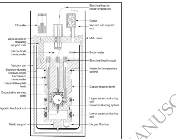
The first iGravs were introduced about 10 years ago and since then approximately 45 iGrav SGs have been manufactured. During this time, several modifications were made to the iGravs to improve their performance. Early iGrav bodies (serial no. 001 to 020) were made shorter than previous SG bodies to reduce Dewar height and weight so as to increase portability. The shorter body reduced the length of the Niobium shield and its shielding effectiveness (sensor design illustrated in Fig. A1, Appendix and Hinderer et al., 2015). As a result, magnetic signals produced by building elevators or nearby parked cars were observed in early iGravs. To remedy this problem, a lead shield was added outside of the vacuum can so that it enclosed the open end of the Niobium shield. Although this proved effective, iGrav bodies (serial no. 021) returned to the original SG design and as a result their Dewars are 10 cm taller; and have a larger volume and hold time for liquid helium during transport. iGrav015 was also retrofitted into a larger Dewar.
ORIGINAL UNEDITED MANUSCRIPT
An additional change that was implemented for serial no. 015, 017 and above, was the introduction of side coils and ‘flux trapping’ to raise the frequency of the commonly observed orbital sphere resonance (Hinderer et al., 2015) out of the long-period seismic band. To accomplish this, four small side coils were placed at sphere height with their axes perpendicular to the axis of the levitation magnets. These were wired so that a current through the coils produced a dipole magnetic field in the vicinity of the sphere, coils, and shield. This change results in the ability to trap the magnetic flux in the sphere, coils and shield, by a specific procedure called ‘flux trapping’. ‘Flux trapping’ consisted of heating the body to 32K (well above Tc), applying a current to the side coils, activating
the getter to add helium gas to the vacuum can to cool the sensor to 4K, and turning off the current. The use of trapped flux was very effective at raising the mode frequency and no abnormal drifts have been reported for dozens of iGravs operated for many years at stationary observatories.
2.2 Co-located gravity measurements at the gravimetric observatory J9 in Strasbourg
J9 has been a gravimetric observatory since 1971 (Rosat et al., 2015; Arnoso et al., 2014). We installed our three iGravs within 2 to 10 meters from each other at J9, where they were operating for up to four months between June and October 2017. Figure 1 shows the positions of the iGravs and of the other gravity meters at the observatory. iOSG023 has been recording at J9 since February 2016 and, therefore, provides good reference for our instruments (Rosat and Hinderer, 2018). Operational setup is shown in the Appendix (Fig. A2).
ORIGINAL UNEDITED MANUSCRIPT
Figure 1. Site map of the underground observatory J9 with the positions of the three iGravs (006, 015, 032) and the observatory instruments (iGrav029, iOSG023) included in this study (modified from Hinderer et al., 2018).
2.3 Remote operation at a geothermal field in North Iceland
On 04 December 2017, we started recording with the gravity meters at Þeistareykir in North Iceland (Fig. 2). iGravs 006 and 032 were set up inside the geothermal field within two kilometres of each other. iGrav015 was initially located outside the geothermal field, 17 kilometres to the northwest, for reference measurements. In June 2019, we relocated iGrav015 to the central position between iGravs 006 and 032. GPS positions of the four monitoring sites are given in the Appendix (Tab. A1).
ORIGINAL UNEDITED MANUSCRIPT
Figure 2. Location of the geothermal field in North Iceland and positions of the gravity stations for each iGrav, iGrav015 was moved from reference to central station in June 2019 (maps compiled with ArcGIS 10.5.1, map.is/os, UTM Zone 28N).
All monitoring sites have similar configuration (Fig. A3, Appendix). They comprise an isolated container with two rooms, each housing a circular concrete pillar. Both pillars are decoupled from the container and attached to the subsurface (bedrock where possible). The continuously operating gravity meter is set up on the pillar in the rear room. The pillar in the entrance room is used for performing calibration measurements with an absolute gravity meter. Each container is equipped with a heater and air conditioning system to keep a constant room temperature of approximately 16°C. A remotely operated multi-parameter station (ROMPS) (Schöne et al., 2013) outside the container monitors hydro-meteorological parameters including barometric pressure, air temperature, precipitation, wind speed, soil moisture and soil temperature. Snow weight, snow height and snow water equivalent are monitored at the east station (iGrav032) only. At every gravity station, we deployed geodetic GNSS receivers for continuous
ORIGINAL UNEDITED MANUSCRIPT
observations of ground motion. Three cameras at each site allow visual inspections of the surroundings and estimation of snow heights at the container corners.
2.4 Instrument transport and timeline of gravity measurements
Figure 3 summarises the different periods of gravity measurements performed at the J9 observatory in Strasbourg and the Icelandic remote monitoring sites in Þeistareykir. Each change of location of a particular instrument marks a transport and may influence the subsequent gravity records. At the end of October 2017, we removed the three iGravs from the measuring site in Strasbourg for transport to Iceland. Transport from J9 to Þeistareykir is illustrated in the Appendix (Fig. A4).Typically, SGs are transported at room temperature without liquid helium inside the Dewar of the gravity meter, and several weeks are required to cool the system to operating temperature (4K) for helium liquefaction and filling. For our study, we targeted to transport the iGrav Dewars at 4K with liquid helium filled (cold transport marked grey in Fig. 3) to avoid the time-consuming cooling phase and the associated generation of significant initial drift rates. Only iGrav006 was transported at room temperature and had to be cooled down to 4K before the start of measurements at J9. For iGrav015 and iGrav032 we successfully realised cold transport for every transport from GWR / San Diego, USA to J9 (truck and airfreight) and J9 to Iceland (truck and ship’s freight). At Þeistareykir iGrav006 had to be re-cooled from only slightly increased temperature (8K) after cold transport. This results from the larger Dewar volumes and associated longer helium hold times for 015 and 032 compared to 006.
We noticed that two of the instrumental iGrav parameters (i.e. noise and drift) are directly dependent on the sensor preparation procedures for cold transport. It turned out that high-temperature annealing before transport causes a reduction in mode frequency and a reduction of drift rates observed for iGrav015 and iGrav032 at the remote monitoring sites, discussed in detail in sections 4 and 5.
ORIGINAL UNEDITED MANUSCRIPT
Figure 3. Timeline of gravity measurements at J9 (Strasbourg, France) and Þeistareykir (Iceland) with the following operating periods at J9: 21.09.2017-23.10.2017 for iGrav006, 21.06.2017-24.10.2017 for iGrav015, 17.06.2017-29.08.2017 and 28.09.2017-24.10.2017 for iGrav032; periods of cold transport at 4K (CT; marked grey) occurred in September 2017 when iGrav032 had to be sent to GWR (San Diego, USA) for maintenance and in November 2017 when all three iGravs were shipped to Iceland; last line shows AG measurements performed with the FG5#206 at J9 and Þeistareykir; FG5 values from January 2018 (dashed margins) are not included in this study because of large measuring uncertainties due to increased ground vibration in the Icelandic winter.
3 Calibration factors
Every iGrav needs a scale factor to convert the measured output feedback voltage to gravity units. We used two methods for estimating the scale factor from the local tidal signal, calibrating the iGrav measurements with either an absolute gravity meter (AG calibration) (Crossley et al., 2018; Riccardi et al., 2012) or side-by-side measurements with an accurately calibrated relative gravity meter (RG calibration) (Hinderer et al., 2015; Meurers, 2012).
For AG calibration, the absolute gravity meter is positioned next to the SG. The AG drop values (in nm s-2) are then least-squares fitted to the SG output voltage to calculate the scale factor (in nm s-2 V-1) (Hinderer et al., 2015). Results from AG calibration using FG5#206 at J9 and Þeistareykir are shown in Table A2 in the Appendix. Uncertainty values of the AG calibrations are up to 3.3 times larger for the Icelandic remote monitoring sites than at J9. One possible reason are the different solid Earth tidal amplitudes (511.6 nm s-2at J9 and 356.1 nm s-2 at Þeistareykir during AG calibration in June/July 2017), leading to increased AG calibration uncertainties in Iceland by a factor 1.4 (40% increase) assuming a linear dependence of the uncertainties to tidal amplitude. As another possible reason we suspect increased local noise at the remote sites from wind, breaking ocean waves, tectonic and geothermal activities, which is negatively
ORIGINAL UNEDITED MANUSCRIPT
affecting AG measurements. In particular, noise from geothermal activities is likely at the iGrav032 and iGrav006 sites due to their short distances to the geothermal well pads.
For RG calibration, a relative gravity meter with known calibration (e.g. by former AG calibration) is positioned next to the SG. Then, analogous to AG calibration both sets of measurements are compared and the data is fitted by a least-squares adjustment from one instrument to the other (Hinderer et al., 2015; Riccardi et al., 2012). We performed RG calibration using one of the observatory superconducting gravity meters (iOSG023) at J9 for all three iGravs in October 2017. The iGrav scale factors obtained by RG calibration at J9 are given in Table A3 in the Appendix. The results shown in Tables A2 and A3 reveal that AG and RG calibrations are very similar and that the uncertainties of RG calibrations are much smaller. However, for a fair comparison between RG and AG calibration factors, one has to consider the absolute calibration uncertainty of the reference gravity meter (2 nm s-2 V-1 for iOSG023).
Due to the lack of AG calibration for iGrav006 at J9 and for iGrav032 at Þeistareykir as well as the increased absolute calibration uncertainties for the remote sites, we consider an alternative approach to determine the scale factor stability after transport to Iceland. Instead of comparing the individual iGravs 006, 015 and 032 to either iOSG023 or FG5#206 we compare them to each other using their RG calibrations determined at J9 (from Tab. A3) as reference. The resulting scale factors are shown in Table 2. To determine the scale factors for Þeistareykir we used iGrav data sets of 8 days in June/July 2019. During this period, iGrav015 was located on the second pillar of the central station (cf. Fig. 2) at about 0.7 km distance to iGrav006 and 1.0 km distance to iGrav032. The increasing distances between the instruments may explain the scale factor differences between J9 and Þeistareykir, with smallest differences for the iGrav006-iGrav015 pair located closest to each other (Fig. 2 and Tab. 2, cols. 7 and 8). To correct for the different locations and elevations of the three iGravs at Þeistareykir, we calculate the scale factors between theoretical tides, using Wahr-Dehant-Defraigne (WDD) solid Earth tides (Dehant et al., 1999) and ocean tide loading (FES2014b; Carrere et al., 2015) models for each of the iGrav locations and multiply the scale factors in column five by this correction factor. As shown in column 11, the differences of the RG calibrations observed between J9 and Þeistareykir are reduced to less than or equal
ORIGINAL UNEDITED MANUSCRIPT
0.01% when taking into account the tidal correction. We conclude that the RG calibrations have not changed after transport, within 0.01% uncertainty.
Table 2. Stability of iGrav scale factors determined by RG calibration between iGrav pairs before and after transport to Iceland; column 1 shows the iGrav for which the scale factors are calculated using the respective iGrav in column 2 (calibrated to iOSG023, Tab. A3) as reference; columns 3 to 6 show the
resulting scale factors (SF) and standard deviations (SD) for J9 and Þeistareykir; column 8 shows the
distances (Dist.) between each iGrav pair; column 9 shows the correction factors (CF) due to the tides in order to account for the different geographical locations between the iGravs and column 10 shows the therewith corrected scale factors (SFC) for Þeistareykir; columns 7 and 11 show the percentage differences (SFD) between the J9 and Þeistareykir (geographically corrected, SFDC) scale factors.
iGrav pair Scale factor DIFF Geographic correction DIFF
J9 Þeistareykir J9-Þei Þeistareykir J9-Þei
1 Obj 2 Ref 3 SF nms-2 V-1 4 SD nms-2 V-1 5 SF nms-2 V-1 6 SD nms-2 V-1 7 SFD % 8 Dist. km 9 CF 10 SFC nms-2 V-1 11 SFDC % 006 015 -914.29 0.0040 -914.24 0.0032 0.0055 0.66 1.00012 -914.35 0.0065 006 032 -914.23 0.0075 -914.01 0.0055 0.0241 1.64 1.00021 -914.20 0.0031 015 006 -930.11 0.0041 -930.16 0.0032 0.0054 0.66 0.99988 -930.05 0.0066 015 032 -930.14 0.0067 -929.97 0.0051 0.0183 1.00 1.00009 -930.05 0.0093 032 006 -895.77 0.0074 -895.98 0.0054 0.0234 1.64 0.99979 -895.79 0.0024 032 015 -895.85 0.0065 -896.02 0.0050 0.0190 1.00 0.99991 -895.94 0.0100
The stability of calibration factors examined above can also be considered with regard to the change of the local value of g between J9 and Þeistareykir. A more detailed description and related calculations for the ‘variation of SG calibration caused by change in latitude or elevation’ are given in the Appendix.
4 Noise analyses
A combination of instrumental noise (e.g. data acquisition noise or sphere resonance effects; Rosat et al., 2015; Imanishi, 2005) and/or environmental noise (of e.g. seismic or meteorological origin) may limit the precision with which gravity signals of interest can be measured. We expect lower environmental noise to be present at a quiet, isolated site like J9 in Strasbourg, compared to an active geothermal site like Þeistareykir. In addition, we expect to observe larger gravity signals (ocean load and waves) at the
ORIGINAL UNEDITED MANUSCRIPT
Icelandic remote sites, due to their short distance to the coastline (8 km for the reference station). In this study, we applied the three-channel correlation method (TCCM) initially proposed by Sleeman et al. (2006) and adapted to SGs by Rosat and Hinderer (2018) in order to extract the incoherent noise (containing the iGrav self-noise) from ambient noise common to the three channels (here instruments). This method consists of calculating the Power Spectral Densities (PSDs) and cross-spectra of calibrated gravity records from three SGs applying a modified smoothed Welch periodogram estimator. We used calibrated gravity signals in nm s-2 with 1 Hz sampling rate from which we compute the PSDs. As a consistent time-window for all monitoring sites, we chose gravity records of seven days during ‘quiet’ periods (no obvious earthquakes or other disturbances).
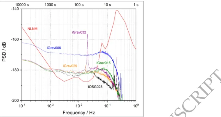
For J9 a direct comparison of the three iGravs is severely limited by the short record length of iGrav006 (cf. Fig. 3). Instead, we compare each of the three iGravs independently to two SGs (iGrav029 and iOSG023) which were continuously recording during our observation period at J9. We chose records from 20.08.2017 to 26.08.2017 for iGravs 015 and 032, and from 03.10.2017 to 09.10.2017 for iGrav006. As shown in Figure 4, iGrav015 and iGrav032 have average self-noise levels of -180 dB at intermediate frequencies (from 10-3 to 10-1 Hz) similar to those of iGrav029 and iOSG023, and in consistence with the observations from Rosat and Hinderer (2018) of low self-noise levels for different iGravs at J9. Only iGrav006 shows about 10 dB higher self-noise. Most likely, this increased noise of iGrav006 is a consequence of improper alignment of the coldhead isolation frame, so that the coldhead is in contact with the inside of the Dewar neck and vibrations from the coldhead are being directly transmitted to the gravity sensor. The sharp peaks at higher frequencies (between 100 and 350 mHz) have also been observed for other SGs at J9 (Rosat and Hinderer, 2018) but the cause has not been identified yet.
ORIGINAL UNEDITED MANUSCRIPT
Figure 4. The instrument-specific noise levels resulting from the three-channel correlation method (TCCM) applied on 1-second data (1 Hz) of iGravs 006, 015 and 032 during seven ‘quiet’ days at J9 in comparison to iGrav029 and iOSG023; Noise levels computed as Power Spectral Densities (PSD) relative
to 1 (m s-2)2 Hz-1; New Low Noise Model (NLNM; Peterson, 1993) shown for reference.
For Þeistareykir we chose records from 15.07.2019 to 21.07.2019, after relocation of iGrav015 to the central station, to directly apply the TCCM to the nearby located iGravs. The results from Þeistareykir (Fig. 5) show similar self-noise between -180 and -170 dB among the three iGravs. Compared to J9 we observe slightly increased noise levels by approximately 5 dB for iGravs 015 and 032 at the remote stations. At frequencies around 0.2 Hz we observe microseismic peaks (up to -165 dB), which do not appear in the PSDs from J9. This is likely caused by incoherent microseismic signals between the sites at Þeistareykir. We must note that in the TCCM, we assume that the ambient environmental noise is common to the three instruments. Since the three iGravs are located at different positions within the geothermal field, with slightly different environmental conditions, the self-noise extraction is less efficient than at J9, where the three gravity meters are collocated within a few meters. As a result, cancellation of environmental noise between the remote stations is less efficient in the TCCM. Non-coherent part of the environmental noise will remain and be interpreted as instrumental noise, which could lead to the increased self-noise observed for the remote stations.
ORIGINAL UNEDITED MANUSCRIPT
Another observation is that the microseismic peak for iGrav015 is about 3 to 4 dB lower than for iGrav006 and iGrav032. Possible reasons could be the slightly different response functions or the larger calibration uncertainties among the iGrav pairs containing iGrav015 (Tab. 2, col. 11). It could also be caused by differences from the iGrav remote installations. For example, the terrain at the central station (iGrav015) is characterised by higher amounts of bedrock than the west and east stations, which may favour a better decoupling for the iGrav pillar and thus less microseismic noise being transmitted to iGrav015.
Figure 5.The instrument-specific noise levels resulting from the three-channel correlation method (TCCM) applied on 1-second data (1 Hz) of iGravs 006, 015 and 032 during seven ‘quiet’ days at the three remote stations within the Þeistareykir geothermal field; Noise levels computed as Power Spectral Densities
(PSD) relative to 1 (m s-2)2 Hz-1; New Low Noise Model (NLNM; Peterson, 1993) shown for reference.
At frequencies around 10-2 Hz (between 9 and 20 mHz), the graphs show distinct spikes, visible in the plots for J9 and Þeistareykir (Figs. 4 and 5). This effect has been called ‘the parasitic mode’ (Van Camp, 1999; Richter et al., 1995) and is due to horizontal displacements of the sphere that turn into an orbital mode (Hinderer et al., 2015). At J9 we note sphere parasitic resonance at 20 mHz for iGrav032 (Fig. 4). At Þeistareykir the orbital mode frequencies of iGrav015 and iGrav032 are reduced to about 9 mHz (Fig. 5) because both sensors were heated above 32K at J9 before shipment to Iceland (see
ORIGINAL UNEDITED MANUSCRIPT
also discussion about high-temperature annealing in section 5). Note that during the three-channel correlation process, the cross-PSD of two instruments is subtracted from the third one resulting in the contamination to all PSDs by these parasitic peaks.
5 Instrumental drift
Every relative gravity meter, including SGs, is characterised by a distinctive instrumental drift behaviour. Drift functions for most SGs are normally toward increasing gravity and combine exponential components that decay with time constants from weeks to months, with a small linear term that varies from 16 to 49 nm s-2 per year for nine SGs operating in Europe (Hinderer et al., 2015; Crossley et al., 2004). This transient drift behaviour can be described as:
g = g + ae + bt (1)
with gravity (g), time (t), the exponential terms (a and k) and the linear term (b).
To identify the instrumental drift of the three iGravs we removed the tidal signals, as well as the effect of air masses (barometric admittance) from the calibrated gravity time series. As a standard tool for gravity reduction, we applied tidal modelling (Agnew, 2015; Merriam, 1992; Francis and Mazzega, 1990) to determine the residual time series for each monitoring site. For computation of local tidal models and the barometric admittance, we used the program ANALYZE from the ETERNA 3.4 package (Wenzel, 1996).
From our measurements at J9, we calculated the gravity residuals by reduction of local tidal parameters and atmospheric admittance factors available from long-term gravity analysis at the observatory (Calvo et al., 2016; Calvo et al., 2014). Figure 6 shows a comparison of the three iGravs and iOSG023 residual time series at J9. For further reduction of the remaining gravity effects including local hydrology, we subtracted the residual (reference) signal of iOSG023 from the iGrav residuals shown in Figure 7. It is noticeable that the iGrav time series are much smoother than in Figure 6 because most of the higher frequency gravity changes are present in all four gravity signals (of iOSG023, iGrav006, iGrav015 and iGrav032) and hence disappear in the difference. To
ORIGINAL UNEDITED MANUSCRIPT
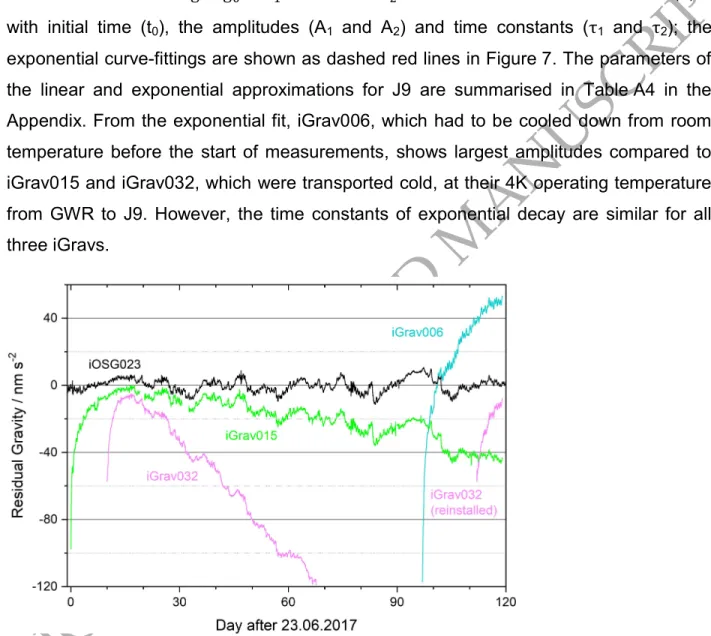
isolate the initial exponential drift and quantify the linear long-term component we applied a linear drift correction for iGrav015 and iGrav032 (dashed black lines in Fig. 7). The time series of iGrav006 and iGrav032 after reinstallation (after day 90 in Fig. 6) were too short to apply linear drift corrections. We calculated the linear term by:
g = g + 𝑥𝑡 (2)
with initial gravity at t = 0 (g0) and the drift rate (x). As approximation for the initial drift,
we used a two-term exponential decay function:
g = g + A e ( )/ + A e ( )/ (3) with initial time (t0), the amplitudes (A1 and A2) and time constants (τ1 and τ2); the
exponential curve-fittings are shown as dashed red lines in Figure 7. The parameters of the linear and exponential approximations for J9 are summarised in Table A4 in the Appendix. From the exponential fit, iGrav006, which had to be cooled down from room temperature before the start of measurements, shows largest amplitudes compared to iGrav015 and iGrav032, which were transported cold, at their 4K operating temperature from GWR to J9. However, the time constants of exponential decay are similar for all three iGravs.
Figure 6. Time series from J9, showing gravity residuals of iOSG023, iGrav006, iGrav015 and iGrav032 after reduction of local tides and atmospheric pressure effects.
ORIGINAL UNEDITED MANUSCRIPT
Figure 7. Time series from J9, showing gravity differences to the reference iOSG023 and subsequent linear drift correction for iGrav015 (dark green) and iGrav032 (purple), no linear drift corrections were done for iGrav006 and the reinstalled iGrav032 (after day 90 in Fig. 6) because of too short time series; dashed lines show linear (black) and exponential (red) curve-fittings for drift estimation; exponential fit for iGrav006 is extrapolated for days 120 to 137.
At Þeistareykir, the gravity monitoring sites are located at distances of several kilometres to each other (up to ~2 km at the geothermal field and ~17 km apart from iGrav015). For this reason, satisfactory reduction of site-dependent gravitational effects like solid Earth tides or ocean loading cannot be achieved by calculating gravity differences between two instruments as at J9 (in Fig. 7), where the gravity meters were installed inside the same building. Instead, we calculated local tidal models for each of the remote monitoring sites and used them for reduction of the iGrav time series.
Figure 8 shows the iGrav residual time series for the first 18 months of observation at the Þeistareykir remote monitoring sites. For instrumental drift characterisation, we used AG measurements (Hinderer et al., 2015) from two FG5#206 campaigns at Þeistareykir in June/July 2018 and June 2019. With the FG5 measurements as benchmark, we corrected the long-term linear drift of each iGrav. After AG correction, we used Eq. 3 to approximate the initial transient drift. The parameters for the linear and exponential corrections are summarised in the Appendix (Tab. A5). Out of the three instruments, only iGrav006 shows the initial exponential behaviour as observed from the
ORIGINAL UNEDITED MANUSCRIPT
measurements at J9. At the Icelandic remote monitoring site, however, the exponential component of the iGrav006 residuals has smaller amplitude and time constants and is visible only for a few days after installation (see also Fig. A5, Appendix).
Figure 8. Time series from Þeistareykir, showing gravity residuals of the 3 iGravs (bright colours), long-term drift estimations by comparison to FG5#206 absolute measurements in summer 2018 and summer 2019 (red dots with error bars) and the resulting drift corrected iGrav residuals (bold colours).
A comparison of the linear long-term drift rates for J9 and Þeistareykir is shown in Table A6 in the Appendix. The results from J9 show negative drift rates of -137 nm s-2 per year for iGrav015 and -837 nm s-2 per year for iGrav032. After transport to Iceland, we observe reduced negative drift rates of -92 nm s-2 per year for iGrav015 and -597 nm s-2 per year for iGrav032, and a positive drift rate of +70 nm s-2 per year for iGrav006.
From our observations at J9 and Þeistareykir, only iGrav006 shows the expected drift behaviour of an initial transient function followed by a small linear term. The drift curves observed for both iGrav015 and iGrav032 were anomalous and can be described by a transient decay toward increasing gravity followed by a much larger negative drift. The problem was most likely caused by shipping iGravs 015 and 032 after side coils had been used to trap flux in the sphere, coils and shield. GWR attempted to remove the trapped flux from both iGravs by heating the sensors inside the vacuum can (above 32K)
ORIGINAL UNEDITED MANUSCRIPT
and letting them slowly recool to 4K, before shipment to Iceland. In later analysis, it was realised that this high-temperature annealing would generally reduce the magnitude of the negative drift but would not eliminate it completely. In retrospect, it could have been more beneficial to warm these two iGravs to room temperature, subsequently recool to 4K at J9, and then activate them in Iceland without using the side coils.
The drift rates of iGrav015 and iGrav032 both decreased after transport to Iceland (Tab. A6, Appendix). This reduction in drift rate most likely indicates that the high- temperature annealing of the sensor at J9 was effective. However, it has not been proven that the negative anomalous drift magnitude is linear. An alternative explanation is that the negative drift could also have an exponential component and that its magnitude slowly decreased in the time elapsed between operation at J9 and installation in Iceland.
6 Conclusions
We analysed continuous gravity measurements of three superconducting iGravs before and after transport to remote monitoring sites. We focused our investigation on calibration, noise and drift, and the influence of transport on these instrumental parameters. For calibration, we used AG (FG5#206) and RG (iOSG023) calibration methods. The stability of the AG calibration factors after transport from J9 to Þeistareykir was limited to 0.64% uncertainty, presumably by high noise disturbances on the AG measurements, from the nearby operating well pads at Þeistareykir. In contrast, the stability of the RG calibration factors was determined to better than 0.01%. For noise analyses, we used a three-channel correlation method. The comparison of noise levels confirms that the iGravs show resonance effects of the sphere and indicate a possible minor change of the iGrav self-noise of about 5 dB after transport to Iceland, although field conditions are also different from the conditions at J9. We estimated the instrumental drift by linear and exponential fitting of the iGrav time series. The results show that there is an exponential component, which presumably started after first initialisation of the iGravs. For iGrav006 (smaller Dewar and no side coils), the initial transient behaviour is also visible at Þeistareykir, which could have started after the
ORIGINAL UNEDITED MANUSCRIPT
sensor warmed up to 8K during shipment to Iceland. For iGravs 015 and 032 which both have side coils we observe negative drifts after preparing and transporting at 4K (cold transport). The cause of the negative drifts is not yet understood. In fact, iOSG023, which has side coils, was also transported cold from GWR to J9 and its drift curve conforms to typical drift behaviour expected with SGs. Negative drifts have been observed not only in shipping iGravs from GWR to J9, and from J9 to Iceland, but also from GWR to other locations. The problem was diagnosed and removed from other iGravs (by warming the sensors to room temperature and re-cooling to 4K) about one year after the start of installations in Iceland. For the three sites in Þeistareykir, we plan further AG campaigns to validate and improve the long-term drift characterisation.
Our analyses revealed that:
1. Calibration is not affected by transport,
2. Noise is dependent on local conditions mostly, with only minor changes of the iGrav self-noise after transport,
3. Initial transient drift is reduced when the SGs are transported cold, but long-term drift rates cannot be transferred from one site to another without validation by repetitive AG measurements.
Our findings from the comparison measurements at J9 and the first results from the remote sites at Þeistareykir provide a promising basis for continuation of the long-term monitoring of the geothermal field. Further comparison to time-lapse micro-gravimetry carried out at Þeistareykir (Portier et al., 2020), is planned to improve the understanding of the general spatial distribution of the gravity changes within the geothermal field.
Acknowledgments
We thank Landsvirkjun the Icelandic National Power Company for providing the necessary facilities and infrastructure at the Þeistareykir geothermal field and for their great ongoing support for installation and servicing of the gravity stations. We gratefully acknowledge GWR Instruments, Inc. for numerous hours of work during installation and operation of the iGravs and additionally providing iGrav015 to improve the comparability of our measurements. Many thanks to Hreinn Hjartarson, Richard Reineman,
ORIGINAL UNEDITED MANUSCRIPT
Stephan Schröder, Tania Ballerstedt, Marvin Reich, Nico Stolarczuk, Julia Illigner, Cornelia Zech, Felix Rietz, Henning Francke and Frederic Littel for their keen help during installation, transport and reinstallation of the gravity meters. We also thank Jean-Daniel Bernard for performing the FG5 absolute measurements at J9 and Þeistareykir, and we acknowledge funding from LABEX ANR-11-LABX-0050\G-EAU-THERMIE-PROFONDE managed by the French National Research Agency. Funding for this project was provided by the German Federal Ministry for Education and Research (BMBF, grant: 03G0858A), the Helmholtz Centre Potsdam GFZ German Research Centre for Geosciences and Landsvirkjun. Prof. Duncan Agnew, Walter Zürn and an anonymous reviewer are gratefully acknowledged for their constructive comments and improvements to the manuscript.
ORIGINAL UNEDITED MANUSCRIPT
References
Agnew, D.C., 2015. Earth Tides, in Treatise on Geophysics, vol. 3 Geodesy, second edition, vol. ed. T. Herring, ed. in chief Schubert G., Elsevier, Amsterdam, The Netherlands, 151-178, https://doi:10.1016/b978-0-444-53802-4.00058-0.
Amalvict, M., Hinderer, J., Boy, J.P. & Gegout, P., 2001. Three Year Comparison Between a Superconducting Gravimeter (GWR C026) and an Absolute Gravimeter (FG5# 206) in Strasbourg (France), Journal of the Geodetic Society of Japan, 47(1), 334-340, https://doi.org/10.11366/sokuchi1954.47.334.
Arnoso, J., Riccardi, U., Hinderer, J., Córdoba, B. & Montesinos, F.G., 2014. Analysis of co-located measurements made with a LaCoste&Romberg Graviton-EG gravimeter and two superconducting gravimeters at Strasbourg (France) and Yebes (Spain), Acta Geodaetica et Geophysica, 49(2), 147-160, https://doi.org/10.1007/s40328-014-0043-y.
Calvo, M., Hinderer, J., Rosat, S., Legros, H., Boy, J.-P., Ducarme, B. & Zürn, W., 2014. Time stability of spring and superconducting gravimeters through the analysis of very long gravity records, J. of Geodyn., 80, 20-33, https://doi.org/10.1016/j.jog.2014.04.009.
Calvo, M., Rosat, S. & Hinderer, J., 2016. Tidal spectroscopy from a long record of superconducting gravimeters in Strasbourg (France), in: Freymueller J.T., Sánchez L. (eds) International Symposium on Earth and Environmental Sciences for Future Generations. International Association of Geodesy Symposia, vol 147. Springer, Cham, https://doi.org/10.1007/1345_2016_223.
Carbone, D., Poland, M.P., Diament, M. & Greco, F., 2017. The added value of time-variable microgravimetry to the understanding of how volcanoes work, Earth-Science Reviews, 169, 146-179, https://doi.org/10.1016/j.earscirev.2017.04.014.
Carbone, D., Cannavò, F., Greco, F., Reineman, R. & Warburton, R.J., 2019. The benefits of using a network of superconducting gravimeters to monitor and study active volcanoes, Journal of Geophysical Research: Solid Earth, 123, https://doi.org/10.1029/2018JB017204.
Carrere, L., Lyard, F., Cancet, M. & Guillot, A., 2015. FES 2014, a new tidal model on the global ocean with enhanced accuracy in shallow seas and in the Arctic region.
ORIGINAL UNEDITED MANUSCRIPT
EGUGA, April 2015, Vienna, id.5481.Crossley, D., Hinderer, J. & Boy, J.P., 2004. Regional gravity variations in Europe from superconducting gravimeters, Journal of Geodynamics, 38(3-5), 325-342, https://doi.org/10.1016/j.jog.2004.07.014.
Crossley, D., Calvo, M., Rosat, S. & Hinderer, J., 2018. More Thoughts on AG–SG Comparisons and SG Scale Factor Determinations, Pure and Applied Geophysics, 175(5), 1699-1725, https://doi.org/10.1007/s00024-018-1834-9.
Dehant, V., Defraigne, P. & Wahr, J.M., 1999. Tides for a convective Earth. Journal of Geophysical Research: Solid Earth, 104(B1), 1035-1058., https://doi.org/10.1029/1998JB900051.
Fores, B., Champollion, C., Le Moigne, N., Bayer, R. & Chery, J., 2017. Assessing the precision of the iGrav superconducting gravimeter for hydrological models and karstic hydrological process identification, Geophysical Journal International, 208(1), 269-280, http://dx.doi.org/10.1093/gji/ggw396.
Francis, O. & Mazzega, P., 1990. Global charts of ocean tide loading effects, Journal of Geophysical Research: Oceans, 95(C7), 11411-11424, https://doi.org/10.1029/JC095iC07p11411.
Güntner, A., Reich, M., Mikolaj, M., Creutzfeldt, B., Schroeder, S. & Wziontek, H., 2017. Landscape-scale water balance monitoring with an iGrav superconducting gravimeter in a field enclosure, Hydrol. Earth Syst. Sci., 21, 3167-3182, https://doi.org/10.5194/hess-21-3167-2017.
Harnisch, G. & Harnisch, M., 2006. Hydrological influences in long gravimetric data series, Journal of Geodynamics, 41(1-3), 276-28, https://doi.org/10.1016/j.jog.2005.08.018.
Hinderer, J., Crossley, D. & Warburton, R.J., 2015. Superconducting gravimetry, in Treatise on Geophysics, vol. 3 Geodesy, second edition, vol. ed. T. Herring, ed. in chief Schubert G., Elsevier, Amsterdam, The Netherlands, 66–122, https://doi.org/10.1016/B978-0-444-53802-4.00062-2.
Hinderer, J., Rosat, S., Schäfer, F., Riccardi, U., Boy, J.-P., Jousset, P., Littel, F. & Bernard, J.-D., 2018. Intercomparison of a dense meter-scale network of superconducting gravimeters at the J9 gravimetric observatory of Strasbourg, France,
ORIGINAL UNEDITED MANUSCRIPT
1st Workshop on the International Geodynamics and Earth Tide Service (IGETS), Potsdam, Germany, June 2018.
Imanishi, Y., 2005. On the possible cause of long period instrumental noise (parasitic mode) of a superconducting gravimeter, Journal of Geodesy, 78(11-12), 683-690, https://doi.org/10.1007/s00190-005-0434-5.
Jacob, T., Chery, J., Bayer, R., Le Moigne, N., Boy, J.-P., Vernant, P. & Boudin, F., 2009. Time-lapse surface to depth gravity measurements on a karst system reveal the dominant role of the epikarst as a water storage entity, Geophysical Journal International, 177(2), 347-360, https://doi.org/10.1111/j.1365-246X.2009.04118.x.
Jousset, P., Mori, H. & Okada, H., 2000. Possible magma intrusion revealed by temporal gravity, ground deformation and ground temperature observations at Mount Komagatake (Hokkaido) during the 1996–1998 crisis, Geophysical Journal International, 143(3), 557-574, https://doi.org/10.1046/j.1365-246X.2000.00218.x.
Kennedy, J., Ferré, T.P.A., Güntner, A., Abe, M. & Creutzfeldt, B., 2014. Direct measurement of subsurface mass change using the variable baseline gravity gradient method, Geophysical Research Letters, 41, 8, 2827-2834, https://doi.org/10.1002/2014GL059673.
Kennedy, J., Ferré, T.P.A. & Creutzfeldt, B., 2016. Time‐lapse gravity data for monitoring and modeling artificial recharge through a thick unsaturated zone, Water Resources Research, 52(9), 7244-7261, https://doi.org/10.1002/2016WR018770.
Melchior, P., 1974. Earth tides, Geophysical surveys, 1(3), 275-303, https://doi.org/10.1007/BF01449116.
Merriam, J.B., 1992. Atmospheric pressure and gravity, Geophysical Journal International, 109(3), 488-500, https://doi.org/10.1111/j.1365-246X.1992.tb00112.x.
Meurers, B., 2012. Superconducting gravimeter calibration by colocated gravity observations; results from GWR C025, International Journal of Geophysics, 2012, 1-12, http://dx.doi.org/10.1155/2012/954271.
ORIGINAL UNEDITED MANUSCRIPT
Peterson, J., 1993. Observations and Modelling of Seismic Background Noise, Open-File Report 93-332, U.S. Department of Interior, Geological Survey, Albuquerque, NM.
Portier, N., Hinderer, J., Drouin, V., Sigmundsson, F., Schäfer, F., Jousset, P., Erbas, K., Magnusson, I., Hersir, G.P., Águstsson, K., De Zeeuw Van Dalfsen, E., Guðmundsson, Á. & Bernard, J.-D., 2020. Time-lapse Micro-gravity Monitoring of the Theistareykir and Krafla Geothermal Reservoirs (Iceland), submitted: Proceedings World Geothermal Congress, Reykjavik, Iceland.
Riccardi, U., Rosat, S., Hinderer, J., Wolf, D., Santoyo, M.A. & Fernandez, J., 2012. On the accuracy of the calibration of superconducting gravimeters using absolute and spring sensors; a critical comparison, Pure and Applied Geophysics, 169(8), 1343-1356, http://dx.doi.org/10.1007/s00024-011-0398-8.
Richter, B., Wenzel, H.-G., Zürn, W. & Klopping, F., 1995. From chandler wobble to free oscillations: comparison of cryogenic gravimeters and other instruments in a wide period range, Phys. Earth Planet. Inter., 91, 131-148, https://doi.org/10.1016/0031-9201(95)03041-T.
Rosat, S., Calvo, M., Hinderer, J., Riccardi, U., Arnoso, J. & Zürn, W., 2015. Comparison of the performances of different spring and superconducting gravimeters and STS-2 seismometer at the gravimetric observatory of Strasbourg, France, Studia Geophysica Et Geodaetica, 59(1), 58-82, http://dx.doi.org/10.1007/s11200-014-0830-5.
Rosat, S. & Hinderer, J., 2018. Limits of Detection of Gravimetric Signals on Earth, Scientific reports, 8(1), 15324, https://doi.org/10.1038/s41598-018-33717-z.
Schilling, M. & Gitlein, O., 2015. Accuracy estimation of the IfE gravimeters Micro-g LaCoste gPhone-98 and ZLS Burris Gravity Meter B-64, in IAG 150 Years. Springer, Cham., 143, 249-256, https://doi.org/10.1007/1345_2015_29.
Schöne, T., Zech, C., Unger-Shayesteh, K., Rudenko, V., Thoss, H., Wetzel, H-U., Gafurov, A., Illigner, J. & Zubovich, A., 2013. A new permanent multi-parameter monitoring network in Central Asian high mountains – from measurements to data bases, Geosci. Instrum. Method. Data Syst., 2, 97-111, https://doi.org/10.5194/gi-2-97-2013.
ORIGINAL UNEDITED MANUSCRIPT
Sleeman, R., Van Wettum, A. & Trampert, J., 2006. Three-channel correlation analysis: A new technique to measure instrumental noise of digitizers and seismic sensors, Bulletin of the Seismological Society of America, 96(1), 258-271, https://doi.org/10.1785/0120050032.
Van Camp, M., 1999. Measuring seismic normal modes with the GWR C021 superconducting gravimeter, Phys. Earth Planet. Inter., 116, 81-92, https://doi.org/10.1016/S0031-9201(99)00120-X.
Van Camp, M., Hendrickx, M., Richard, P., Thies, S., Hinderer, J., Amalvict, M., Luck, B. & Falk, R., 2003. Comparisons of the FG5# 101,# 202,# 206 and# 209 absolute gravimeters at four different European sites, Cahiers du Centre Européen de Géodynamique et de Séismologie, 22, 65-73.
Van Camp, M. & Francis, O., 2007. Is the instrumental drift of superconducting gravimeters a linear or exponential function of time?, Journal of Geodesy, 81(5), 337-344, https://doi.org/10.1007/s00190-006-0110-4.
Warburton, R.J., Pillai, H. & Reineman, R.C., 2010. Initial results with the new GWR iGravTM superconducting gravity meter, IAG Symposium Proceedings, June 2010, Saint Petersburg, http://www.gwrinstruments.com/pdf/warburton-pillai-reineman-revised.pdf, [last accessed 22-June-2020].
Wenzel, H.G., 1996. The Nanogal software: Earth tide data processing package ETERNA 3.30, Bull. Inform. Marees Terrestres, 124, 9425-9439, http://www.eas.slu.edu/GGP/ETERNA34/MANUAL/ETERNA33.HTM, [last accessed 22-June-2020].
Wilson, C.R., Scanlon, B., Sharp, J., Longuevergne, L., & Wu, H., 2012. Field test of the superconducting gravimeter as a hydrologic sensor, Groundwater, 50(3), 442-449, https://doi.org/10.1111/j.1745-6584.2011.00864.x.
ORIGINAL UNEDITED MANUSCRIPT
Appendix
Variation of SG calibration caused by change in latitude or elevation
For SG levitation, the current in the magnet (Ic) produces induced currents (Ics) in the
sphere. Since Ics is proportional to Ic, the levitation force (FL) is simply expressed as
FL(Ic) = L(Ic)2 = mg, where L depends on the sphere and magnet geometry and is about
2.5 m/s2/A2 for the iGrav, with a levitation current A ≈ 2 A; m is the mass of the sphere and g is the local value of gravity. The feedback force is proportional to the product of the current in the feedback coil (i) and the current in the sphere Ics. Again, since Ics is
proportional to Ic, the feedback force can be expressed as Ffb(i) = BiIc ∝ i√g, with the
constant B = 0.05 m/s2/A2 for a typical iGrav. Therefore, the variation of the iGrav scale factor caused by either a change in elevation or latitude can be calculated by the following formula:
∆C = g
g (A1)
With the absolute gravity values at the station of lowest latitude (J9) g0 = 9.80878 m s-2
and at the station of highest latitude (Þeistareykir, reference station) gn = 9.82312 m s-2.
The resulting scale factor change is 1.00073 (i.e. 0.073%) after transport from J9 to Þeistareykir. This is a larger uncertainty than the 0.01% determined by RG calibration. However, it is still much smaller than the best stability of AG calibration with an uncertainty of 0.64% (6 nm s-2 V-1) obtained for iGrav015 (Tab. A2, Appendix).
ORIGINAL UNEDITED MANUSCRIPT
Figure A1. Schematic of the gravity sensor inside the iGrav Dewar showing arrangement of the sphere, coils and shielding (modified from Hinderer et al., 2015)
(a) (b)
Figure A2. Measuring setup for iOSG023 (a) and iGravs 032 and 015 (b) at the gravimetric observatory J9 in June 2017; with each instrument connected to a separate helium cooling system and data acquisition unit.
ORIGINAL UNEDITED MANUSCRIPT
(a) (b)
Figure A3. Setup of gravity station similar at all four remote sites (here reference station with iGrav015 shown), GNSS and hydro-meteorological parameters measured outside the container (a); measuring setup inside the container with the iGrav installed on a concrete pillar, decoupled from the surroundings and grounded to the bedrock (b).
(a) (b) (c)
Figure A4. Packing and transport of the iGravs with liquid helium filled (4K, cold transport); after securing the Dewar and component parts inside the GWR supplied crates (a and b at J9, Strasbourg), the instruments were transported by truck and ship freight to the remote monitoring sites in Iceland (c).
ORIGINAL UNEDITED MANUSCRIPT
Figure A5. Exponential fit of iGrav006 gravity residuals for the initial 13 days after installation at
Þeistareykir, subsequent to FG5#206 drift correction; fit function: g = g0 - 11e^(-(t - t0) / 0.089) - 62e^(-(t -
t0) / 1.65).
Table A1. Coordinates and heights above sea level for the remote monitoring sites at Þeistareykir, obtained by GPS (Garmin handheld) measurements; iGrav015 moved from reference to central station in June 2019.
Latitude (°) Longitude (°) Height (m a.s.l.)
iGrav006 (west station) 65.8853 -16.9750 332
iGrav015 (reference station) 66.0027 -17.1925 334
iGrav015 (central station) 65.8819 -16.9634 340
iGrav032 (east station) 65.8787 -16.9430 378
ORIGINAL UNEDITED MANUSCRIPT
Table A2. Absolute gravity (AG) calibration with FG5#206; at J9 for iOSG023 (duration of 6.2 days in
September 2016), iGravs 015 and 032 (duration of 7.1 days in July 2017); atÞeistareykir for iGravs 006
and 015 (duration of 5.0 and 4.8 days in June/July 2018); no AG calibrations (X): for iGrav006 at J9 because it was installed in October 2017 when FG5#206 was not available, and for iGrav032 at Þeistareykir because of excessive noise from geothermal well pads during AG measurements at east station; uncertainty of AG calibration factors (from AG-SG least-squares fit) are proportional to uncertainty of the AG drop values (the uncertainty of the SGs being negligible in comparison).
SG name J9 Þeistareykir AG calibration factor nm s-2 V-1 AG calibration factor uncertainty nm s-2 V-1 AG calibration factor nm s-2 V-1 AG calibration factor uncertainty nm s-2 V-1 iOSG023 -451 2 X X iGrav006 X X -917 10 iGrav015 -934 3 -935 6 iGrav032 -898 3 X X
Table A3. Relative gravity (RG) calibration at J9 of iGravs 006, 015 and 032 by fitting to iOSG023; standard deviations (SD) are formal errors for the RG scale factors between iOSG023 and the respective iGrav, smaller than the AG calibration uncertainties because of the large number of SG values sampled at 1 second in the parallel comparison.
SG name Scale factor
nm s-2 V-1 SD nm s-2 V-1 iGrav006 -914.27 0.0042 iGrav015 -930.18 0.0019 iGrav032 -895.84 0.0065
Table A4. Parameters of linear and exponential fitting of iGrav gravity differences from J9.
J9 iGrav006 iGrav015 iGrav032
Value SD Value SD Value SD
Linear fit Drift rate
(nm s-2 d-1) X X -0.375 0.00006 -2.29 0.00039 Exponential fit A1 (nm s-2) -63.7 0.0729 -42.3 0.106 -34.4 0.0734 τ1 (d) 0.616 0.00142 0.870 0.00432 0.744 0.00315 A2 (nm s-2) -93.6 0.0350 -25.2 0.0704 -44.3 0.0621 τ2 (d) 8.31 0.0104 8.67 0.0257 5.67 0.00773
ORIGINAL UNEDITED MANUSCRIPT
Table A5. Parameters of linear and exponential fitting of iGrav gravity residuals from Þeistareykir.
Þeistareykir iGrav006 iGrav015 iGrav032
Value SD Value SD Value SD
Linear fit FG5#206 diff.
(nm s-2) 67 16 51 13 59 24 Drift rate (nm s-2 d-1) +0.19 0.046 -0.25 0.039 -1.6 0.069 Exponential fit A1 (nm s-2) -11 0.59 X X X X τ1 (d) 0.089 0.0085 X X X X A2 (nm s-2) -62 0.23 X X X X τ2 (d) 1.7 0.0080 X X X X
Table A6. Long-term drift rates (in nm s-2 a-1) from linear approximations of time series from J9 and
Þeistareykir.
Location Timeframe iGrav006 iGrav015 iGrav032
J9 120 days for iGrav015 (June - October 2017)
60 days for iGrav032 (July - August 2017)
X X -137 X X -837
Þeistareykir 350 days for each iGrav (June 2018 - June 2019) +70 -92 -597