Handling variability at the code level : modeling, tracing and checking consistency

HAL Id: tel-01720323

https://tel.archives-ouvertes.fr/tel-01720323

HAL is a multi-disciplinary open access archive for the deposit and dissemination of sci-entific research documents, whether they are pub-lished or not. The documents may come from teaching and research institutions in France or abroad, or from public or private research centers.

L’archive ouverte pluridisciplinaire HAL, est destinée au dépôt et à la diffusion de documents scientifiques de niveau recherche, publiés ou non, émanant des établissements d’enseignement et de recherche français ou étrangers, des laboratoires publics ou privés.

and checking consistency

Xhevahire Tërnava

To cite this version:

Xhevahire Tërnava. Handling variability at the code level : modeling, tracing and checking consistency. Software Engineering [cs.SE]. Université Côte d’Azur, 2017. English. �NNT : 2017AZUR4114�. �tel-01720323�

Université Côte d’Azur

DOCTORAL SCHOOL STIC

ET DE LA COMMUNICATION

P H D T H E S I S

to obtain the title of

PhD of Science

of the Université Côte d’Azur

Specialty : C

S

Defended by

Xhevahire T

ËRNAVA

Handling Variability at the Code Level: Modeling,

Tracing and Checking Consistency

Thesis Advisor: Philippe C

CNRS, I3S, Sophia Antipolis, France

defended on 01 December 2017

Jury :

Olivier BARAIS - Professor, Université de Rennes 1 Reviewer Mireille BLAY-FORNARINO - Professor, Université Côte d’Azur Examiner Philippe COLLET - Professor, Université Côte d’Azur Advisor Laurence DUCHIEN - Professor, Université de Lille Examiner Tewfik ZIADI - Associate Professor, HDR, UPMC - LIP6 Reviewer

Université Côte d’Azur

ECOLE DOCTORALE STIC

ET DE LA COMMUNICATION

Thèse de doctorat

Présentée en vue de l’obtention du grade de

docteur en Sciences

de l’Université Côte d’Azur

Mention : I

Présentée et soutenue par

Xhevahire T

ËRNAVA

Gestion de la Variabilité au Niveau du Code :

Modélisation, Traçabilité et Vérification de

Cohérence

Dirigée par: Philippe C

CNRS, I3S, Sophia Antipolis, France

Soutenance prévue le 01 décembre 2017

Devant le jury composé de:

Olivier BARAIS - Professeur des Universités, Rennes 1 Rapporteur Mireille BLAY-FORNARINO - Professeur des Universités, Côte d’Azur Examinatrice

Philippe COLLET - Professeur des Universités, Côte d’Azur Directeur

Laurence DUCHIEN - Professeur des Universités, Lille Examinatrice

Abstract. When large software product lines are engineered, a combined set of traditional techniques, such as inheritance, or design patterns, is likely to be used for implementing variability. In these techniques, the concept of feature, as a reusable unit, does not have a first-class representation at the implementation level. Further, an inappropriate choice of techniques becomes the source of vari-ability inconsistencies between the domain and the implemented variabilities.

In this thesis, we study the diversity of the majority of variability implementa-tion techniques and provide a catalog that covers an enriched set of them. Then, we propose a framework to explicitly capture and model, in a fragmented way, the variability implemented by several combined techniques into technical variability models. These models use variation points and variants, with their logical relation and binding time, to abstract the implementation techniques.

We show how to extend the framework to trace features with their respective implementation. In addition, we use this framework and provide a tooled ap-proach to check the consistency of the implemented variability. Our method uses slicing to partially check the corresponding propositional formulas at the domain and implementation levels in case of 1–to–m mapping. It offers an early and auto-matic detection of inconsistencies.

As validation, we report on the implementation in Scala of the framework as an internal domain specific language, and of the consistency checking method. These implementations have been applied on a real feature-rich system and on three product line case studies, showing the feasibility of the proposed contribu-tions.

Résumé. Durant le développement de grandes lignes de produits logiciels, un ensemble de techniques d’implémentation traditionnelles, comme l’héritage ou les patrons de conception, est utilisé pour implémenter la variabilité. La no-tion de feature, en tant qu’unité réutilisable, n’a alors pas de représentano-tion de première classe dans le code, et un choix inapproprié de techniques entraîne des incohérences entre variabilités du domaine et de l’implémentation.

Dans cette thèse, nous étudions la diversité de la majorité des techniques d’implémentation de la variabilité, que nous organisons dans un catalogue étendu. Nous proposons un framework pour capturer et modéliser, de façon fragmen-tée, dans des modèles techniques de variabilité, la variabilité implémentée par plusieurs techniques combinées. Ces modèles utilisent les points de variation et les variantes, avec leur relation logique et leur moment de résolution, pour ab-straire les techniques d’implémentation.

Nous montrons comment étendre le framework pour obtenir la traçabilité de feature avec leurs implémentations respectives. De plus, nous fournissons une ap-proche outillée pour vérifier la cohérence de la variabilité implémentée. Notre méthode utilise du slicing pour vérifier partiellement les formules de logique propositionnelles correspondantes aux deux niveaux dans le cas de correspon-dance 1–m entre ces niveaux. Ceci permet d’obtenir une détection automatique et anticipée des incohérences.

Concernant la validation, le framework et la méthode de vérification ont été implémentés en Scala. Ces implémentations ont été appliquées à un vrai système hautement variable et à trois études de cas de lignes de produits.

Acknowledgments

I began this work in the name of God, the Beneficent, the Merciful, and I thank Him for every single progress in my life. Then, many people supported, encouraged, and motivated me, in one way or another, during this work. My sincere thanks to all of them! I shall mention here those who did much more than I expected from them.

I would like to express my nearly boundless gratitude to my supervisor Philippe Collet, who replied to my very first email to him and accepted to super-vise me in this work, even without knowing me. I thank him for his unwavering support, for his readiness, and for all those constructive discussions, which kept me constantly engaged, especially during my research work in the distance. Liter-ally, it was a complete privilege to be mentored by him, and hopefully, our cooper-ation will continue. So, I say to him: "thank you for your continued support, thoughtful guidance, encouragement, the shared knowledge, and wisdom. Above all, thanks for your patience!"

I wish to extend my deep appreciation to the reviewers, Olivier Barais and Tewfik Ziadi, who gave their time and attention to reviewing my manuscript and evaluating my work. I thank Mireille Blay-Fornarino and Laurence Duchien for accepting to be on the jury of my thesis. Also, special thanks go to all anonymous and known reviewers of our published work.

I would really like to thank the French Embassy in Kosovo for awarding me a six months per year scholarship for the Ph.D. studies for four years. Also, I thank Nexhat Humolli for saving my workplace at his company, where I worked part-time during the part-time that I was in Kosovo, for almost the first three years of my Ph.D.

Many thanks to the University of Nice Sophia Antipolis for supporting my Ph.D. in so many ways; especially, by making possible my participation in scien-tific conferences and for granting me a financial support for the three months on the last year. Also, thank you for being in the most amazing city.

Warm thanks to my family for being my biggest supporters, especially during these past four years. I cannot ever say this enough, but "faleminderit për gjithçka"! Also, I thank my closest friends (you know who you are) for their enthusiastic support.

Contents

List of Figures ix

List of Tables xii

Listings xiii

List of Acronyms xvii

Glossary xix

1 Introduction 1

1.1 Context . . . 1

1.1.1 Software Product Line Engineering . . . 1

1.1.2 Software Variability Management . . . 2

1.2 Overview of Challenges and Contributions . . . 4

1.2.1 Challenges. . . 4

1.2.2 Contributions . . . 9

1.2.3 Outline . . . 9

2 Background and State of the Art 11 2.1 Variability Modeling . . . 11

2.2 Variability Implementation . . . 13

2.2.1 Variable Parts in Core-Code Assets. . . 13

2.2.2 Variability Abstractions . . . 14

2.2.3 Variability Implementation Techniques . . . 17

2.3 Variability Management Approaches . . . 17

2.3.1 Variability Traceability . . . 18

2.3.2 Modeling and Tracing the Variability of Core Assets. . . 19

2.3.3 Orthogonal Approaches to Variability Traceability . . . 21

2.3.4 Reverse Engineering Approaches. . . 21

2.4 Automated Analysis of Feature Models . . . 22

2.5 Domain Specific Languages . . . 24

I Design of Variability Models at the Implementation Level 27 3 Diversity in Variability Implementations 29 3.1 Dimensions of Diversity . . . 29

3.1.1 Characteristic Properties of Variable Parts. . . 30

3.1.2 Quality Criteria . . . 33

3.2 Catalog Building Method . . . 37 3.2.1 Covered Techniques . . . 37 3.2.2 Evaluation Process . . . 37 3.2.3 Resulting Catalog . . . 38 3.2.4 Related Work . . . 40 3.3 Choosing a Technique . . . 41 3.3.1 Illustration . . . 41 3.3.2 Discussion . . . 42 3.4 Summary. . . 44

4 Technical Variability Models 45 4.1 Capturing the Variability of Core-Code Assets . . . 45

4.1.1 Imperfectly Modular Variability . . . 45

4.1.2 A Framework for Capturing the Variability . . . 49

4.2 Modeling the Implemented Variability . . . 52

4.2.1 Types of Variation Points . . . 53

4.2.2 Fragmented Variability Modeling . . . 56

4.2.3 Capturing and Modeling the Variability for Reverse Engi-neering . . . 58

4.3 Summary. . . 62

II Usage of Technical Variability Models 65 5 Traceability with Technical Variability Models 67 5.1 A Three Step Traceability Approach . . . 67

5.2 Establishing Trace Links . . . 71

5.3 Summary. . . 71

6 Consistency Checking 73 6.1 Assumptions and Issues of Consistency Checking . . . 73

6.2 Proposed Method . . . 78

6.2.1 Initial Checking . . . 78

6.2.2 Slicing . . . 78

6.2.3 Substitution . . . 81

6.2.4 Assertion. . . 81

6.2.5 Handling 1 – M trace links. . . 83

6.3 Related Work . . . 86

6.4 Summary. . . 87

III Implementation and Validation 89 7 Framework Implementation and Applications 91 7.1 Technical Foundations . . . 91

Contents ix

7.2 Applications . . . 94

7.2.1 Design Evaluation of TVMs . . . 98

7.2.2 Limitations . . . 100

7.3 Summary . . . 101

8 An Implementation of the Consistency Checking Method 103 8.1 Implementation . . . 103 8.2 Applications . . . 105 8.2.1 Evaluation Process . . . 105 8.2.2 Execution Time . . . 110 8.2.3 Limitations . . . 111 8.3 Summary . . . 111 9 Conclusion 113 9.1 On Challenges . . . 113

9.2 On the Scope and Limitations . . . 116

9.3 Future Work . . . 118

A Definitions of Features and Variation Points with Variants 121 B The Developed Case Studies 125 B.1 Summary of Case Studies . . . 125

List of Figures

space and solution space separation for software assets (adapted fromCzarnecki[2005];Pohl et al.[2005, Ch. 2]) . . . 2 1.2 Excerpt of the feature model for the Graph product line . . . 3 2.1 The feature model of the Graph product line . . . 11 2.2 Problem space and solution space for variability modeling

(bor-rowed fromCapilla et al.[2013, Ch. 2]). . . 13 2.3 The vp concept as a) a variable point (i.e., the cx), b) a variable part (i.e.,

the cx with variants). The cxis the common part for variants va, vb, and vc. . . 15 2.4 Illustration of two variability traceability dimensions,

realize/imple-ment and use - the blue links (adapted fromAnquetil et al.[2010]) . . 19 2.5 The relation between the concepts of feature, variation point with

variants and software entities (borrowed fromSvahnberg et al.[2005]) 20 3.1 The FM of Expressions PL . . . 41 4.1 Four features of JavaGeom product line . . . 46 4.2 A detailed design excerpt of JavaGeom product line from the

imple-mentations in Listings 4.1 to 4.4 . . . 46 4.3 A three step framework for variability management of core-code

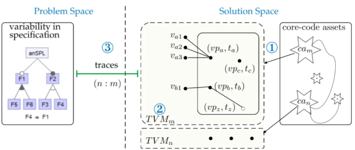
as-sets (T VMm stands for Technical Variability Model (cf. Section 4.2.2) of the core-code asset cam, with vp-s {vpa, vpb, ...} and their respective variants {va1, va2, ...}that are realized by different techniques {ta, tb, ...}. Whereas, {f1, f2, ...}are features in the FM.) . . . 48 4.4 Documentation of the implemented variability in T VMs for the

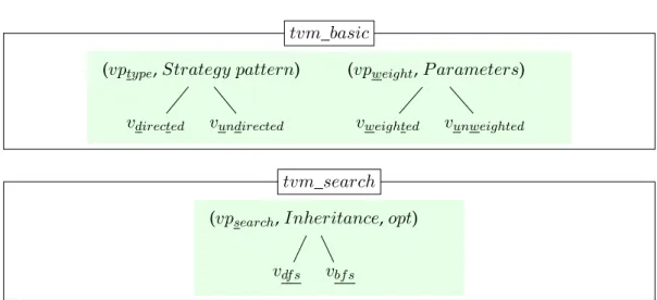
Graph SPL (cf. Figure 2.1) . . . 57 4.5 The reconstructed FM from features in Listing 4.7 . . . 61 5.1 Proposed traceability approach through using the technical

variabil-ity models (TVMs) . . . 68 6.1 A simplified feature model of the Graph PL (cf. Figure 2.1) . . . 74 6.2 Documentation of the implemented variability from Listing 4.5

(Page 55) in TVMs for the Graph PL (cf. Figure 6.1) . . . 75 6.3 Proposed consistency checking method . . . 79 6.4 Consistency checking by asserting the number of configurations . . . 82 6.5 Implementation of vpsearch, from Figure 4.4, as an Or logical relation

between its variants. . . 83 6.6 Example of inconsistency detection . . . 83

6.7 The tvm_search with a technical vp (cf. Figure 4.4 and Figure 6.1) . . 84 6.8 False inconsistency detection for 1 – to – m links . . . 85 7.1 A comparison of TVMs (the colored boxes), and their vp-s with

vari-ants, between the four case studies . . . 95 7.2 The TVMs closer but still separated with the functional code in files . 99 7.3 (a) The separated TVMs in package level; (b) The separated TVMs

in file level; (c) The separated TVMs in package, file, or class level; (d) For example, the TVMs in separate files for Microwave Oven PL. 100 8.1 Prototype toolchain for consistency checking . . . 104 8.2 A setup for checking the consistency of one or several TVMs for

Microwave Oven PL . . . 106 8.3 The detected consistency for a TVM in the Microwave Oven PL . . . 108 8.4 The detected inconsistency for a TVM in the Microwave Oven PL . . 109

List of Tables

2.1 Translation rules from an FM to propositional logic . . . 23

3.1 Logical relations of vp-s and of variants in a vp . . . 31

3.2 Binding times of vp-s with variants (adapted from Bosch and Capilla[2012];Capilla et al.[2013]) . . . 32

3.3 Granularity of vp-s with variants . . . 33

3.4 Quality criteria of variability implementation techniques . . . 34

3.5 Catalog of variability implementation techniques . . . 39

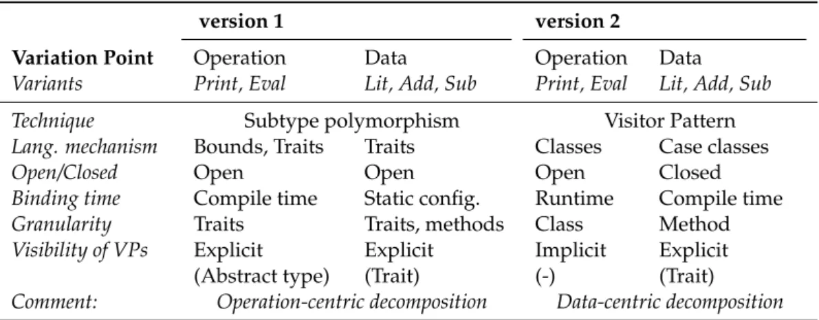
3.6 Two implemented versions of the Expressions PL . . . 42

4.1 Tagging properties of variation points and variants . . . 52

4.2 Types of variation points . . . 53

4.3 Capturing the implemented variability of Graph PL in Listing 4.5 . . 60

4.4 Capturing the implemented variability of Graph PL in Listing 1.1 . . 61

6.1 Features and vp-s with variants configurations in Graph PL . . . 77

7.1 Number of features (F-s), implemented features (Impl. F-s), TVM-s, and the captured vp-s with variants in each case study . . . 96

7.2 Number of vp-s and their implementation techniques in each case study . . . 97

7.3 The documented number of vp-s’ types in each case study . . . 98

8.1 Checking a TVM with one vp and its variants . . . 107

8.2 Checking more than one TVM with one or more vp-s with variants . 107 8.3 Times for checking the consistency of TVMs compared to self-consistency checking of the FM, in the Microwave Oven SPL . . . 110

Listings

(parame-ters and strategy pattern), in the Scala language . . . 4 4.1 An excerpt from the realization of feature StraighCurve2D, for

Jav-aGeom in Figure 4.1, as a variation point AbstractLine2D . . . 47 4.2 An excerpt from the realization of feature Line2D, for JavaGeom

in Figure 4.1, as a variant StraightLine2D of AbstractLine2D . . . 47 4.3 An excerpt from the realization of feature Segment2D, for JavaGeom

in Figure 4.1, as a variant LineSegment2D of AbstractLine2D . . . 47 4.4 An excerpt from the realization of feature Ray2D, for JavaGeom

in Figure 4.1, as a variant Ray2D of AbstractLine2D . . . 47 4.5 The variability on file GraphBasic.scala (given also in Listing 1.1) . . . 55 4.6 The variability on file Search.scala . . . 56 4.7 The Graph SPL using feature modules (borrowed from [Apel et al.,

2013]) . . . 60 7.1 Pattern for defining a variation point and variant. . . 92 7.2 Pattern for modeling some implemented variability in terms of the

defined variation points with variants in Listing 7.1 . . . 92 7.3 Pattern for defining trace links . . . 93 7.4 An excerpt of variability capturing and documentation in JavaGeom 93 7.5 An excerpt of variability traceability in JavaGeom . . . 94 7.6 Defining a nested variation point (a variant becoming a nested vp,

as defined in Section 4.2.1) . . . 94 7.7 An example of multiple trace links, in Microwave Oven PL . . . 96 B.1 Expressions PL implementation - version 1, in Scala language . . . . 128 B.2 Expressions PL implementation - version 2, in Scala language . . . . 129

List of Acronyms

vp Variation Point

CNF Conjuctive Normal Forme CVL Common Variability Language

DM Decision Model

DSL Domain Specific Language

FAMILIAR FeAture Model scrIpt Language for manIpulation and Automatic Reasoning

FM Feature Model

KCVL CVL implementation in Kermeta

MTVM Main Technical Variability Model

OVM Orthogonal Variability Model

SPL Software Product Line

TLs Trace Links

TVM Technical Variability Model

Glossary

JφF MK The set of feature configurations for the FM, φF M

JφM T V MK The set of vp-s with variants configurations for the MTVM, φM T V M BT The set of possible binding times of variation points

EV The evolution properties of variation points

LG The set of possible logical relations of vp-s with variants

T The set of possible traditional variability implementation techniques X The possible types of variation points

φF M The propositional formula for the feature model (FM)

φ0_{F M} The sliced formula of feature model, φF M

φM T V M The propositional formula for the MTVM

φT L The propositional formula for the bidirectional trace links

φ0_{T L} The sliced formula of trace links, φT L

φT V Mx The propositional formula of a specific technical variability model (TVM) core-code assets are those reusable code artifacts that form the basis for eliciting

the software products in a software product line

MTVM The power set of all technical variability models (TVMs) in an SPL

TVMs The technical variability models for modeling the realized variability in core-code assets in a fragmented way

C

1

Introduction

1.1

Context

1.1.1 Software Product Line Engineering

The software product line (SPL) engineering paradigm has emerged to foster methodological reuse between the related software products in a domain or an or-ganization. By adopting it, an organization expects to achieve mass-customization for a family of products, such as decreasing their cost and their time to market while increasing their quality. An SPL is then usually defined as "a set of software-intensive systems sharing a common, managed set of features that satisfy the specific needs of a particular market segment or mission and that are developed from a common set of core assets in a prescribed way [Clements and Northrop,2002;Northrop et al.,2007]. Orig-inally, a feature is defined as "a prominent or distinctive user-visible aspect, quality, or characteristic of a software system or systems"1 _{[Kang et al.,1990] within a domain.} Thus, features are used to describe and scope a set of related software products within a domain through defining their common aspects and their differences.

There are three models for adopting an SPL approach in an organization: proactive, when all products in the scoped domain are preplanned to be built; ex-tractive, when from a set of legacy applications is build/extracted an SPL model; and reactive one, when in either case the SPL itself get evolved [Krueger,2002a]. In addition, the whole development cycle of an SPL consists of (1) domain engi-neering, or development for-reuse, and (2) application engiengi-neering, or develop-ment with-reuse [Cledevelop-ments and Northrop,2002;Kang et al.,1998;Pohl et al.,2005; Weiss et al.,1999]. Despite the SPL adaptation model, domain engineering and ap-plication engineering processes are highly interactive and can occur in any order, which are shown also as rotating cycles byNorthrop et al.[2007].

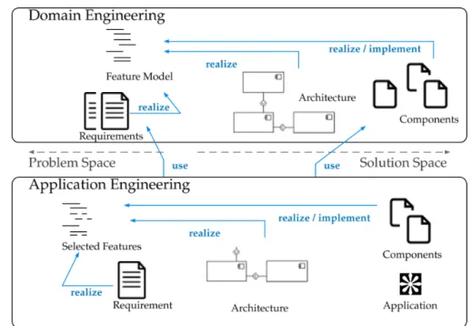
Domain engineering and application engineering. Figure 1.1 shows the do-main engineering and application engineering, as two do-main processes for the de-velopment of software product lines. The domain engineering process is charac-terized by the development of core assets, which represent those reusable artifacts and resources that form the basis for eliciting the single software products during the application engineering process. Core assets are made reusable by modeling and realizing what is common and what is going to vary (i.e., the common and

Figure 1.1: The software product line engineering processes, with the problem space and solution space separation for software assets (adapted fromCzarnecki [2005];Pohl et al.[2005, Ch. 2])

variable features) between the related products in a methodological way. Variabil-ity can be part of any core assets, which "often include, but are not limited to, the architecture, reusable software components, domain models, requirements statements, doc-umentation,..." [Clements and Northrop,2002;Northrop et al.,2007]. In this thesis, in the focus is the variability of core assets at the implementation level, that is, the core-code assets.

Problem space and solution space. Orthogonal with the domain engineering and application engineering is the problem space and solution space dimensions for all software assets [Czarnecki,2005;Czarnecki and Eisenecker,2000, Ch. 3], as is shown inFigure 1.1. While in problem space all valid feature combinations and requirements of software products are specified, in solution space these specifica-tions are realized in concrete software systems, such as their reusable architecture, detailed design, or implementation.

1.1.2 Software Variability Management

An essential activity of the whole product line development is the management activity (cf. Figure 1.1). It can be (1) organizational management, which repre-sents the "authority responsible for the ultimate success or failure of the product line effort" [Northrop et al., 2007], and (2) technical management that deals with the

1.1. Context 3

Figure 1.2: Excerpt of the feature model for the Graph product line

development of core assets and product derivation activities.

Technical management has several practice areas, such as configuration management, make/buy/mine/commission analysis, scoping, tool support, etc. [Clements and Northrop, 2002]. From them, the well-known configura-tion management comes from tradiconfigura-tional single software system development that is extended and represents the variation management in software product lines [Krueger,2002b]. According toKrueger[2002b] andClements and Northrop [2002], variation management is multi-dimensional and basically deals with (1) the variability in space, that is, the management of the variability of core assets at a fixed moment in time, and (2) the variability in time, that is, the management of versions of core assets during the time (as in single software development), maintenance (evolution of domain), and resolution of variability during a prod-uct derivation with different binding times (cf.Section 3.1.1). Thus, variability in space, known as software variability management, is specific only to product lines but, it interferes with the variability in time regarding the binding time, during each product derivation.

In realistic SPLs, where the variability is extensive, a crucial issue is the ability to manage this variability in different core assets and among different abstraction levels [Bosch et al.,2001]. An important aspect of this activity is then the ability to identify or capture and trace a variable unit, commonly known as a feature, in core assets of an SPL. In particular, fromFigure 1.1, the specified domain variability in the problem space needs to be mapped to their respective realization, such as in architecture assets, and core-code assets, in the solution space.

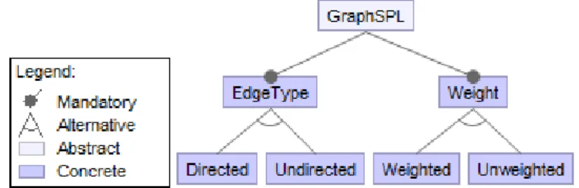
More concretely, the specified domain variability in terms of features is com-monly captured in a variability model (VM), such as a feature model (FM) [Kang et al., 1990] (cf. Figure 1.1). The FM is a tree structure of features, consisting of mandatory, optional, or, and/or alternative logical relations between features with their cross-tree constraints, implies and/or excludes, that are expressed in proposi-tional logic. Semantically, an FM represents the valid software products (i.e., the feature configurations) within an SPL. InFigure 1.2is given an excerpt of the fea-ture model for the Graph product line [Lopez-Herrejon and Batory,2001]2, which is well-known in the academia. Whereas, one of its possible realizations at the

implementation level is also given inListing 1.1.

In this thesis, we address specifically the variability management activities be-tween the specified variability in problem space, for example, the FM inFigure 1.2, and core-code assets in solution space, for example, the implemented variability in Listing 1.1, during the domain engineering process. In this context, we have identified several challenges to be addressed.

1 o b j e c t Conf {

2 f i n a l v a l WEIGHTED: Boolean = t r u e 3 }

4 a b s t r a c t c l a s s Graph { /∗ Core p a r t ∗/ } 5 c l a s s ConcreteGraph extends Graph {

6 def adddirectededge ( s : Vertex , d : Vertex , w: I n t ) = { 7 v a l edge = new Edge ( s , d )

8 i f ( Conf .WEIGHTED) {

9 edge . weight = w

10 }

11 edges = edge : : edges 12 a d d t o a d j a c e n c y m a t r i x ( edge ) 13 }

14 def addundirectededge ( s : Vertex , d : Vertex , w: I n t ) = { 15 v a l edge1 = new Edge ( s , d )

16 v a l edge2 = new Edge ( d , s ) 17 i f ( Conf .WEIGHTED) {

18 edge1 . weight = w 19 edge2 . weight = w

20 }

21 edges = edge1 : : edges 22 edges = edge2 : : edges 23 a d d t o a d j a c e n c y m a t r i x ( edge1 ) 24 a d d t o a d j a c e n c y m a t r i x ( edge2 ) 25 }

26 def addedge ( c a l l b a c k : ( Vertex , Vertex , I n t ) => Unit , 27 x : Vertex , y : Vertex , w: I n t = 1 ) = c a l l b a c k ( x , y , w)

Listing 1.1: Graph PL implementation using two different techniques (parameters and strategy pattern), in the Scala language

1.2

Overview of Challenges and Contributions

We now determine the addressed challenges, then we summarize our contribu-tions and we give an outline of this dissertation.

1.2.1 Challenges

In the described context, there are several challenges to be addressed regarding the modeling and management of variability in core-code assets. These challenges are grouped into three main challenges, as in the following.

1.2. Overview of Challenges and Contributions 5

Challenge A. Variability modeling at the implementation level

A1. Understanding the diversity of variability implementation techniques.

Variability can be implemented by different variability implementation tech-niques, such as inheritance, generic types, design patterns (seeSection 2.2.3). De-pending from the used technique, the units that vary can be diverse at the imple-mentation level. For example, some variability can be implemented at the class level (e.g., using the technique of inheritance), or at method level (e.g., using the technique of overloading). Also, variability can be resolved earlier (e.g., at compile time) or later (e.g., at runtime) during the product derivation. This implies that, when traditional techniques are used (cf.Section 3.1.3), the variability of core-code assets is realized by using a combined set of techniques (e.g., inheritance, overrid-ing, design patterns). In this case, choosing and combining the right techniques to implement some variability of an SPL domain is not trivial. Whereas, when variability is implemented by using a single technique, such as preprocessors in C, the implementation is more straightforward with the whole variability being implemented by using the preprocessor directives.

For evaluating and choosing a technique to address some domain variability at the implementation level, pieces of advice can be found in studies, catalogs, or taxonomies (e.g.,Apel et al.[2013];Bachmann and Clements[2005];Coplien[1999]; Gacek and Anastasopoules[2001];Muthig and Patzke[2003];Patzke and Muthig [2002];Svahnberg et al.[2005]), but their studied techniques are evaluated by dif-ferent subsets of criteria that remain scattered among difdif-ferent research works.

Moreover, towards an approach for documenting the variability at the mentation level, it is necessary to understand the diversity of variability imple-mentation techniques, analysed by the same set of properties. To the best of our knowledge, there is no up-to-date classification and catalog for variability imple-mentation techniques. It is also expected that an enriched catalog would guide the deveopers for choosing the right techniques in the majority of cases.

A2. Capturing and modeling the implemented variability when a combined set of tradi-tional variability implementation techniques is used.

When traditional variability implementation techniques are used to implement some variability, such as inheritance, generic types, or design patterns, the code is not shaped in terms of features from the domain level. Usually, the implemented variability is modeled in terms of variation points (vp-s) with variants [Coplien, 1999; Czarnecki et al., 2012; Jacobson et al., 1997; Schmid and John, 2004] (they are defined inSection 2.2.1). Further, in realistic product lines, variability is im-plemented by using a combined set of such traditional techniques, meaning that the vp-s with variants are diverse (e.g., with different binding times,Section 3.1) compared to the case when a single technique is used to implement the whole variability, for example, by using the preprocessors in C the whole variability is resolved during the compile time in case of a product derivation.

Consequently, the capturing and modeling of the implemented variability in core-code assets when a combined set of traditional variability implementation techniques are used is a challenging task that should be facilitated. Moreover, this modeling phase is essential for managing the variability of core-code assets. A3. Separating the development dimension and variability dimension while maintaining their corresponding relationship (a.k.a. consistency).

Variation points with variants (defined inSection 2.2.1) are not a by-product of the traditional variability implementation techniques [Bosch et al.,2001;Sinnema et al.,2004a], meaning that the places in core-code assets where some variability is realized are implicit. Therefore, the implemented variability needs to be captured and modeled in some way, in order to be managed. The variability of core-code as-sets can become explicit (1) by annotating the places where the variability happens directly in code, for example, using preprocessor directives [Tartler et al., 2012], tags [Heymans et al.,2012], or a visual representation [Kästner,2012], (2) abstract-ing and documentabstract-ing the variability separately from the code, for example, usabstract-ing decisions for variation points with variants in a decision model [Schmid and John, 2003], or (3) implementing/factorizing the code in physically separated modules, for example, in feature modules [Apel et al., 2013]. Here we do not consider the reverse engineering approaches, such as feature location techniques for migrating some related software products in an SPL approach.

Specifically, the development dimension, or the functionality in code, and the variability dimension, or the variability-related issues, can stay either mixed or separated. To ease the variability management, as mentioned byBerg et al.[2005]; John et al. [2007];Muthig and Atkinson[2002], we aim at keeping separated the variability and development dimensions. However, when they are separated, the consistency between the variability dimension and the development dimension becomes an issue as it needs to be maintained; therefore, it is one of our challenges. A4. Modeling the implemented variability in a fragmented way.

In realistic product lines, the number of features in a feature model at the spec-ification level may be considerable (e.g., [Tartler et al.,2012]). On the other hand, the variation points with variants at the implementation level are a refinement of features from the domain level [Hunt and McGregor, 2006]. Consequently, the amount of variability at the implementation level is expected to be even larger than the variability at the domain level [Pohl et al., 2005, Ch. 4]. The capturing and modeling of the implemented variability at once and in one place may then be harder and will weaken, instead of supporting, the management of variability. For such reason, the documentation of the implemented variability in a fragmented way can be practical and helpful, as is suggested by the variability-aware mod-ule system [Kästner et al.,2012] where each implemented module defines its own variability model.

object-1.2. Overview of Challenges and Contributions 7

oriented or functional ones) there is no concept of modules that can be considered as fragments with variability, but variability may happen, for example, within a package, file, or class. Therefore, we aim at modeling the variability of core-code assets in a fragmented way, where a fragment can be flexible, such as a package, file, or class with some variability that is worth to be modeled separately.

Challenge B. Variability traceability

B. Supporting the variability traceability between the specification and implementation levels.

Originally, in the FORM method [Ch. 8Capilla et al.,2013;Kang et al.,1998], the need to model separately the variability at the specification and realization lev-els is already present. While the variability at the realization level is more about the software variability, the specification one represents the variability between the software products themselves within an SPL [Metzger et al., 2007]. In most variability management approaches, it is up to the reader to understand whether a variability model is used to describe the variability at the specification or real-ization levels [Metzger and Heymans,2007]. Moreover, the mapping of features to variable units in implementation is mostly 1 – to –1, for example, between features and preprocessor directives in C [Le et al.,2013;Lotufo et al.,2010;Tartler et al., 2012], although a directive can be scattered in core-code assets. In such cases, the FM is used to model only the implemented variability, or from both levels into a single model. In reality, the mapping of features from the specification level to their implementation is n – to – m [Pohl et al.,2005, Ch.4], and also the variability abstractions in both levels may use different names.

Therefore, an approach for tracing the specified and implemented variabilities, when a combined set of techniques are used, is needed. Moreover, these trace links make possible the variability management and can also be used for other purposes, for example, to resolve the implemented variability during a product derivation, or to check its consistency.

Challenge C. Consistency checking of variability

C1. Checking the consistency of variability between the specification and implementation levels.

According to a recent survey about consistency checking in SPL engineering, by Santos et al. [2015], there are three major approaches to address consistency issues: (1) within the variability models (i.e., FMs), (2) between the FM and other software models, or (3) between the FM and its implementation (i.e., core-code assets). These also correspond to the locations where inconsistencies can happen, as mentioned byVierhauser et al.[2010].

Currently, the support for checking variability consistency between an FM and core-code assets is limited. This means that the specified variability in terms of

features at the domain level and their respective implementation, using the tradi-tional techniques, in core-code assets must represent the same number of software products.

Checking the consistency between the implemented and specified variabilities is also a challenging task, as the mapping of the specified features in an FM to the core-code assets is n – to – m. But, we expect to check their variability consistency within the context of their trace links.

C2. Checking the consistency of variability when a combined set of traditional variability implementation techniques is used.

The existing approaches are mostly conceived for resolving inconsistencies within a specific software, such as the Linux kernel [Lotufo et al., 2010; Tartler et al., 2012], or when the variability is implemented by a single variability im-plementation technique, for instance, using preprocessors in C [Le et al., 2013]. However, in realistic SPL settings, variability is implemented by using a combined set of traditional techniques, such as inheritance, overloading, design patterns. An inappropriate choice and combination of such techniques become the source of variability inconsistencies that cannot be detected by existing approaches. In this work, we consider that the variability of core-code assets is implemented by using a combined set of traditional techniques.

In case that some variability is implemented by using an improper technique, several inconsistencies may appear, for example, when an alternative logical rela-tion between features in a variability model is implemented by a variarela-tion point, with an Or logical relation between its variants. In such case, the number of pos-sible products at the specification level is inconsistent with the pospos-sible products that can be derived from the core-code assets. Therefore, in complement to Chal-lenge C1, a consistency checking approach should be able to check whether the right technique to implement some variability is used.

C3. Achieving an early detection of variability inconsistencies.

The consistency of some specified variability can be checked only after it is real-ized in core-code assets, but not necessarily only after the whole specified variabil-ity is addressed. Commonly, some variabilvariabil-ity is deferred to be implemented later or during the application engineering phase. In addition, it becomes harder to fix the inconsistencies after all of them are shown at the same time at the end [Vier-hauser et al.,2010]. In particular, it has been shown that trying to change the im-plementation technique for some addressed variability, only after the whole SPL is implemented, can be very costly [Bachmann and Clements, 2005]. Therefore, an approach for detecting earlier the variability inconsistencies is needed, for ex-ample, to be able to select a single or a group of variation points with variants and to check them against the specified features at the domain level early during the development process. Typically, we could expect that the earlier a variability inconsistency is identified, the cheaper becomes the fix.

1.2. Overview of Challenges and Contributions 9

1.2.2 Contributions

In this dissertation, we address these challenges by offering a detailed and tooled framework for modeling and managing the variability of core-code assets. Specif-ically, our contributions can be summarized as follows.

A catalog of variability implementation techniques. First, we study the diver-sity for the majority of the existing variability implementation techniques and provide a unified set of comparison criteria for them. Then, we build a cat-alog that covers an enriched set of techniques, which are compared by using the same set of criteria.

A framework for modeling and tracing the variability of core-code assets. We used the analysed diversity of variability implementation techniques to create our framework for capturing and modeling the variability of core-code assets. Specifically, the framework supports the capturing and modeling of variabil-ity when a combined set of traditional variabilvariabil-ity implementation techniques are used at the implementation level, which exposes a form of what we de-fine as imperfectly modular variability. Moreover, the framework is based on capturing or abstracting the variability implementation techniques, with their characteristic properties, in terms of variation points with variants, which are used for modeling the variability of core-code assets into so-called technical variability models, in a fragmented way.

In addition, the framework supports traceability, by defining the n–to–m trace links between the features in a feature model at the domain level and the vari-ation points with variants in technical variability models at the implementa-tion level.

A method for checking the consistency of the implemented variability.Through modeling the variability in a fragmented way, we provide a method for check-ing the consistency between the specified and implemented variabilities, as earlier during the realization of core-code assets. Concretely, the method uses a slicing technique over the variability models to partially check the corre-sponding propositional formulas at the domain and implementation levels in case of their 1–to–m mapping.

Tool support and validation.Finally, we present a concrete implementation of our framework as an internal DSL in the Scala language. Further, we use this DSL for implementing the method for variability consistency checking. Both these implementations are applied on a real feature-rich system and on three prod-uct line case studies, showing the feasibility of the proposed contributions.

1.2.3 Outline

In the following, Chapter 2gives a background for the used concepts in this thesis, and the state of the art in variability management, which is not specific to core-code assets. An introduction on domain specific languages (DSL), as a mean for

building tool support in variability modeling is also given. Our contribution is then presented, organized in three parts.

Part I: Design of variability models at the implementation level. In this part, Chapter 3presents the studied diversity of variability implementation techniques, an updated catalog of them, and shows a way for using the catalog during the eval-uation and choice of techniques. InChapter 4we describe our framework for cap-turing and modeling the imperfectly modular variability (defined inSection 4.1.1) at the implementation level. Also, the importance of capturing the variability im-plementation techniques during a reverse engineering process.

Part II: Usage of technical variability models. Chapter 5proposes an extension of the framework, for tracing the specified and implemented variabilities under their n–to–m trace links. Chapter 6describes the method for checking the consis-tency of the variabilities between the specification and implementation levels. Part III: A tool support. In Chapter 7 an implementation of the framework, as a domain specific language, is presented, as well as its usage in four case stud-ies. Similarly, Chapter 8presents a concrete implementation of the consistency checking method and reports on it application in four case studies.

Finally, Chapter 9 concludes the thesis by summarizing the addressed chal-lenges, and gives some further perspectives and our future work.

C

2

Background and State of the Art

This chapter is an introduction to the main topics and related approaches of this thesis. Specifically, we introduce variability modeling in Section 2.1, variability realization at the implementation level inSection 2.2, and variability traceability as a key aspect for variability management of core-code assets inSection 2.3. Then, we discuss automated analysis of feature models in Section 2.4, as a means for automatic consistency checking of variability, Section 2.5is dedicated to domain specific languages as a support for tooling the approach proposed in this thesis.

2.1

Variability Modeling

Since its first presentation byKang et al.[1990], feature modeling (FM) is widely adopted as a means for documenting the commonalities and variabilities in terms of features of software products in an SPL. In different approaches or usage con-texts, a feature is defined. Appendix Agives 20 of its definitions. Similarly, the original notion of feature model has been extended over time.Capilla et al.[2013, Ch. 2] compares 11 FM variations (by Benavides et al. [2005]; Czarnecki et al. [2002]; Czarnecki and Eisenecker [2000]; Czarnecki et al. [2004]; Eriksson et al. [2005];Griss et al.[1998];Hein et al.[2000];Kang et al.[1998];Riebisch et al.[2002]; Van Gurp et al.[2001] ), and a more holistic approach to feature modeling is also available [Lee et al.,2014].

Figure 2.1: The feature model of the Graph product line

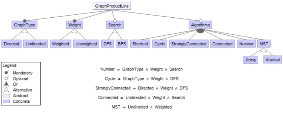
As an illustration, a concrete feature model, the Graph PL, is given inFigure 2.1. This SPL is quite well understood and used by the community [Lopez-Herrejon and Batory, 2001]. It is a hierarchically arranged set of features with the main

feature, GraphProductLine, representing conceptually the SPL domain. It has two compound mandatory features,GraphTypeandWeight, with their alternative variant features, «Directed,Undirected» and «Weighted,Unweighted», respec-tively. Also, it has two compound optional features, Search and Algorithms. The first one has two alternative variant features, «DFS, BFS», and the second one has six features in an Or relation, «Shortest, Cycle, StronglyConnected, Connected,Number, andMSTwith alternative featuresPrimeandKruskal». Fea-tures in an FM can have cross-tree constraints, which are commonly expressed in propositional logic. This Graph PL has five cross-tree constraints, such asNumber → (GraphType∧Weight∧Search), meaning that the selection of featureNumber requires featuresGraphType,WeightandSearchto be selected.

Thus, the software variability of an SPL is documented in a variability model (VM), which is commonly expressed as a feature model (FM) [Kang et al., 1990], but it can also be a decision model (DM) (first introduced by the Synthesis method [Corporation,1993;Schmid et al.,2011]), an orthogonal variability model (OVM) [Pohl et al.,2005], or FMs complemented by a Domain Specific Language (DSL) [Voelter and Visser,2011]. The FM and DM were introduced almost at the same time and used quite equally [Czarnecki et al.,2012]. According to the Synthe-sis method, "a Decision Model identifies, for each work product family, the application engineering requirements and engineering decisions that determine how members of the work product family can vary" [Corporation, 1993]. Overall, any variability model (FM, DM, etc.) can be considered as a decision model whenever it is used for tak-ing the decisions durtak-ing the product derivation [Capilla et al.,2013, Ch. 20]. While the variability in an FM has a graphical representation, in a DM it has a tabular representation [Dhungana and Grünbacher,2008;Forster et al.,2008;Muthig and Atkinson,2002;Schmid and John,2004]. Besides, there are also formal approaches for transforming an FM to a DM and vice versa [El-Sharkawy et al.,2012].

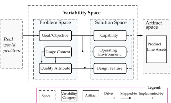
Problem space and solution space variability. Similar to the problem and so-lution space for core assets, given inSection 1.1.1[Czarnecki,2005;Czarnecki and Eisenecker,2000;Turner et al.,1999], the problem space and solution space for vari-ability are distinguished [Ch. 2Capilla et al.,2013;Lee et al.,2014]. This variability space is given inFigure 2.2, which shows that, depending on the viewpoints, fea-tures can be in problem variability space (i.e., goal/objective, usage context, and quality attribute features) or solution variability space (i.e., capability, operating environment, and design features). The approach byMetzger et al. [2007] recog-nizes these two variability spaces as the product line (PL) variability and software variability.

There are few approaches that distinguish clearly these two variability spaces. Their difference is introduced earlier in the FORM method [Kang et al.,1998] then, among the first, in the variability management approach by Becker[2003a,b]. In the majority of other approaches, it is up to the reader to understand when an FM represents the PL variability or the software variability [Metzger and Heymans,

2.2. Variability Implementation 13

Figure 2.2: Problem space and solution space for variability modeling (borrowed fromCapilla et al.[2013, Ch. 2])

2007].

According to a study by Czarnecki et al.[2012], an FM is mainly used at the specification level for scoping the software products within an SPL in terms of features, whereas a DM is used closer to the realization level (i.e., architecture, implementation, etc.) for supporting the resolution of variation points (vp-s) with variants in form of decisions (their definition is given inSection 2.2.1). In our work, we consider specifically the implementation level (i.e., the core-code assets).

2.2

Variability Implementation

2.2.1 Variable Parts in Core-Code Assets

In realistic SPL settings, the implementation of variability in core-code assets com-plies, mostly, to a commonality and variability approach, despite the program-ming paradigm (e.g., object-oriented, or functional) [Coplien,1999]. Specifically, a domain is decomposed into subdomains, then within each subdomain the com-monality is factorized from the variability that is used to differentiate the software products within the domain.

The core-code assets consist of three parts: the core, commonalities, and vari-abilities. The core part is what remains of the system in the absence of any particu-lar feature [Turner et al.,1999], that is, the assets that are included in any software product of the SPL. A commonality is a common part for the related variant parts within a subdomain. After the commonality is factorized from the variability and

implemented it becomes part of the core (i.e., it is buried in the core [Coplien, 1999]), except when it represents some optional variability. The variant parts are used to distinguish the software products in the domain. A subdomain can have more than one common and variant part. The core with the commonalities and variabilities of all subdomains constitute the wholeness of core-code assets in an SPL.

The commonalities and variabilities in core-code assets are commonly stracted in terms of variation points (vp-s) with variants, as solution oriented ab-stractions. Unlike features in problem space, vp-s with variants are related to con-crete elements in core-code assets. Originally, "a variation point identifies one or more locations at which the variation will occur" [Jacobson et al.,1997]. Respectively, vari-ation points are known as a manifestvari-ation of variability in architecture, in design, and, eventually, in implementation [Fritsch et al., 2002]. The way that a varia-tion point is going to vary is expressed by its variants. Over time, several other definitions of vp-s with variants have appeared (see 16 of their definitions in Ap-pendix A).

The variable part is like an organizing container. It contains the location where some variability happens in core-code assets (i.e., the variation point), the variants, and the used technique to implement them.

2.2.2 Variability Abstractions

In order to understand in terms of what abstractions we should capture some im-plemented variability, we analyse in this section the usage of features and varia-tion points (vp-s) with variants in the literature. In the following, we show their definitions as problem or solution oriented abstractions, the diversity of their ter-minology, and the different meanings of a vp concept.

Problem or solution oriented abstractions. To understand whether the concept of features or vp-s with variants are used solely as problem oriented or solution oriented variability abstractions, we analysed their definitions in 34 approaches (seeAppendix A).

We compared 20 definitions of the feature concept, also analysed byClassen et al.[2008],Patzke et al.[2011], andApel et al.[2013, Ch. 2]. From them, eleven definitions consider a feature as a problem oriented abstraction (including the orig-inal definition byKang et al.[1990]), four of them as a solution oriented abstraction (including the extension of the original definition [Kang et al.,1998]), and five are general definitions. Apel et al. [2013] give explicitly a broader (i.e., more inclu-sive) definition of a feature by subsuming the variability of problem and solution spaces.

Similarly, we analysed 14 definitions of the variation point. Twelve of them em-phasize that a vp is a solution oriented concept (including the original definition by Jacobson et al.[1997]), a single one uses the notion of variable part in solution space instead of the variation point [Bachmann and Clements,2005], and the last

2.2. Variability Implementation 15 cx va vb vc ... a) cx va vb vc ... b)

Figure 2.3: The vp concept as a) a variable point (i.e., the cx), b) a variable part (i.e.,

the cxwith variants). The cxis the common part for variants va, vb, and vc.

one defines it as a problem oriented concept [Pohl et al.,2005]. In a subsequent ap-proach [see Metzger et al.,2007],Pohl et al.[2005] make even clearer the usage of vp-s only as domain abstractions. Although, in the standard [ISO/IEC 26550:2015, 2015], byPohl et al.[2005], the feature concept is also defined and used as a prob-lem oriented abstraction.

In two definitions of vp, the abstractions of feature and variation point are used together. The first one considers that an FM is also a core asset and a vp is used to point the varying places in the FM [Czarnecki and Eisenecker,2000]. The sec-ond definition, byHunt and McGregor[2006], stresses that vp-s are refinements of features.

Naming. In the literature, features and vp-s with variants are sometimes called differently. Mostly, the alternative names for features reflect their usage as problem or solution oriented abstractions. For example, a feature is known as a delivery unit, configuration unit, reuse unit, semantic unit (in problem space), or as syn-tactic unit [Kästner et al.,2011], design decision (design feature), changeable deci-sion (alternative design feature) [Capilla et al.,2013], variation point feature [Griss, 2000], or variant feature (in solution space). On the other hand, a vp is known as a design decision, delayed design decision [Van Gurp et al., 2001], spot [Becker, 2003a], extension point [Apel et al.,2013], or generic element [Becker,2003b].

Sometimes, the notions of feature and vp with variants are used alternatively. For example, in problem space, the node at which varying features are attached (i.e., the compound feature) is known as vp [Czarnecki and Eisenecker,2000;Griss, 2000]. In solution space, a design feature is the vp and an alternative design feature (or variant feature) is the variant [Capilla et al.,2013].

Semantics of variability abstractions. Variability abstractions in problem space, such as features, are mere names which are not related to any variability realiza-tion technique or core asset in realizarealiza-tion levels. On the contrary, vp-s and solurealiza-tion space features are related to a concrete variability implementation technique or a varying element within core-code assets, that is, they concretely point the elements of core-code assets that are going to vary. For example, a solution space feature can point to a file [Beuche et al.,2004], a feature module in Feature-Oriented program-ming [Apel et al.,2013], or a macro in C using its preprocessors [Kästner,2012]. Similarly, a vp can be a (super) class, an interface, a parameter [Jacobson et al., 1997], or an #ifdef in C [Schmid and John,2004].

Mostly, a vp is understood as (1) a handle for relating the specified variabil-ity to its respective varying element(s) in core assets on realization levels [CVL, 2012], (2) an abstraction of a location or point that vary in core-code assets (cf. Figure 2.3a) [Jacobson et al., 1997], (3) a variable part (cf. Figure 2.3b) [Bach-mann and Clements, 2005], (4) an abstraction of a variability implementation technique [Capilla et al., 2013, pg. 48], or (5) as the symmetry (i.e., common-ality invariance) and symmetry breaking places in software [Coplien and Zhao, 2000]. Regarding the first meaning, in a prototype implementation of the CVL, KCVL [Barais et al.,2013; KCVL,2015], is stated that "Using variation points, it is possible to express and manipulate the links between the variability abstraction model and the base model". Although the vp is used here as a link, it also supports some se-mantics for reassigning references or excluding its other related model elements from the base model. The third, fourth, and fifth meanings are related, as the com-monality is factorized by using a variability implementation technique, whereas the technique represents the mechanism to accommodate the variants and thus to resolve the variability. In addition, most of the traditional variability imple-mentation techniques have the properties of the symmetry or symmetry break-ing in software [Castellani,2003;Coplien and Zhao,2000;Rosen,1995;Zhao and Coplien,2003, 2002]. In geometry, the symmetry is defined as the immunity to a possible change [Rosen,1995]. Whereas, in software, a symmetry can be identified between a class in object-oriented (which can be a vp) and its objects (its variants). Specifically, a class establishes an invariance relationship between the class and its objects, which are analogue (i.e., changed but still the same) with respect to the class structure [Coplien and Zhao,2000].

Independent from the implementation technique. There are approaches for managing the implemented variability in terms of features (e.g., [Apel et al.,2013; Heymans et al., 2012; Kästner and Apel, 2009]) and those in terms of variation points with variants (e.g., [Becker,2003b;Capilla et al.,2013;Jacobson et al.,1997; Pohl et al.,2005;Schmid and John,2004]). Thereby, in the literature, both abstrac-tions of feature and vp are used almost equally and sometimes in combination.

We observed that the differences between a feature and a vp oriented imple-mentation are not related to a specific variability impleimple-mentation technique. In most cases, a vp with variants are implemented by a traditional technique such as inheritance, parameterization, etc. On the other hand, there are approaches where a feature represents a class, a file [Beuche et al.,2004] or a plugin. As another exam-ple, forThüm et al.[2014] preprocessors are used as a technique for implementing features, whereas bySchmid and John[2004] they are used as a technique for im-plementing vp-s. But, still, the concepts of features and vp-s with variants are not the same thing that is just called differently in different approaches.

An essential difference. Basically, the concept of a feature is used to annotate or put in a separate module all those lines of code that may belong to a specific

fea-2.3. Variability Management Approaches 17

ture (e.g., [Apel et al.,2013;Heymans et al.,2012;Kästner,2010;Lee et al.,2000]). Whereas, a vp is used as a way for abstracting a varying place without making a commitment about which lines of code are exactly in or out the vp concept. Specif-ically, in our understanding, a vp with variants represents some entities that have a fuzzy border in core-code assets.

In this work, unless explicitly specified, we consider that variation points with variants are solution oriented abstractions that we use for capturing and managing the variability in core-code assets, whereas features as problem oriented abstrac-tions.

2.2.3 Variability Implementation Techniques

The techniques that are used for realizing the variability in an SPL are called vari-ability realization techniques [Capilla et al.,2013;Svahnberg et al.,2005], variabil-ity mechanisms [Bachmann and Clements,2005;Jacobson et al.,1997;Muthig and Patzke,2003], or variability implementation techniques [Fritsch et al.,2002]. Vari-ability realization technique is a general term used for techniques acting at the archi-tecture, design, or code level; whereas, the term variability implementation technique will be only used for techniques at the code. All variability implementation tech-niques came from several programming paradigms and are supported by different constructs in different programming languages, which in turn offer different prop-erties.

An SPL is structured around a set of features of several kinds, which repre-sent different functional or non-functional software products’ requirements. These features have to be properly realized and their reflection to vp-s with variants is manifold in architecture, design, and especially in implementation, forming an n-to-m relation [Gacek and Anastasopoules,2001;Metzger and Pohl,2014]. Each vp is associated with one or more variability implementation techniques (e.g., when several implemented versions of the same vp are needed for achieving different binding times [Dolstra et al.,2003a,b;Rosenmüller et al.,2011]) and vice versa. In principle, one vp is associated with only one technique, whereas the same tech-nique can be used to implement several vp-s within a domain. Examples of vari-ability implementation techniques are inheritance in object orientation, preproces-sors, feature modules or some design patterns. In Listing 1.1(Section 1.1.2) we show the usage of parameters and strategy pattern in the Scala language as vari-ability implementation techniques for implementing the two compound features, GraphTypeandWeight, for the Graph PL (cf.Figure 2.1).

2.3

Variability Management Approaches

Variability management is a complex activity, first because variability is realized in different types of core assets (e.g., requirements, architecture, code, etc.) and then, within each of these abstraction levels, different variability realization techniques

can be used. For example, at the requirements or architecture level, various ex-tensions of the UML (Unified Modeling Language) are proposed by using notes or stereotypes [Clauß and Jena,2001;Ziadi et al.,2003;Ziadi and Jézéquel,2006]. Whereas, at the implementation level, with a textual representation, different tex-tual or language annotations [Heymans et al.,2012;Tartler et al.,2012], language constructs [Apel et al., 2013; Schaefer et al.,2010], or visualization tools [Kästner et al.,2008b] are used. Therefore, modeling and tracing the variability of these core assets is a primary step for the variability management during the SPL engineer-ing [Berg et al.,2005].

2.3.1 Variability Traceability

The CoEST 1 [Cleland-Huang et al.,2012] defines a trace (noun 2) as "a specified triple of elements comprising: a source artifact, a target artifact, and a trace link associating the two artifacts". And, the traceability as "the potential for the traces to be established and used".

The concept of traceability is already used for different reasons in single (tradi-tional) software engineering, mostly to trace requirements [Winkler and Pilgrim, 2010]. Its meaning and techniques need to be enhanced for use in SPL engineer-ing, because the relevant entities that are required to be traced and the semantics of trace links in SPL engineering and in traditional software engineering are quite different.

Traceability dimensions. Principally, four dimensions of traceability are distin-guished among the literature: horizontal (intra), vertical (inter), versioning, and variability traceability [Anquetil et al., 2008, 2010; Cleland-Huang et al., 2012; Krueger,2002b;Schmid and John,2004;Winkler and Pilgrim,2010]. The first three dimensions are similar as in the traditional software engineering, whereas vari-ability tracevari-ability is specific to SPL engineering and deals with varivari-ability in space (i.e., the variability of core assets in a specific moment of time).

Variability traceability "is dealt by capturing variability information explicitly and modeling the dependencies and relationships separate from other development arti-facts" [Berg et al.,2005]. It has two other dimensions: tracing the realized variabil-ity (i.e., the variabilvariabil-ity from the problem space to the solution space), and tracing the resolved variability (i.e., the software artifacts between application engineering and domain engineering) [Anquetil et al.,2010;Krueger,2002b;Pohl et al.,2005]. They are shown as realize/implement and use trace links, respectively, inFigure 2.4. Further, the term variability traceability is used mostly for the first dimension. The horizontal and vertical traceability came from the single system engineering, but can also have the meaning of tracing the variability in an SPL among the artifacts within the same abstraction level or between different abstraction levels, respec-tively. And, the versioning traceability conducts the evolution of a software artifact

1_{Center of Excellence for Software Traceability:http://coest.org/}

2.3. Variability Management Approaches 19

Figure 2.4: Illustration of two variability traceability dimensions, realize/implement and use - the blue links (adapted fromAnquetil et al.[2010])

(in traditional engineering) and/or the evolution of variability (with the variability in time, in SPL engineering).

All these traceability dimensions are orthogonal to each other: (1) they may in-teract, such that, the variability traceability links may be subject to evolution over time, and (2) can be applied in a hierarchical way, that is, versioning traceability can be applied to variability, inter, and intra traceability, then variability traceabil-ity can be applied to inter and intra traceabiltraceabil-ity [Anquetil et al.,2008].

Usage of trace links. A generic traceability process model comprises the cre-ation, usage, and maintenance of trace links [Gotel et al.,2012], as the trace links are established to meet a specific usage purpose during a software engineering process and need to be maintained. In SPL engineering, variability traceability can be established and used for different reasons, and by different stakehold-ers [Anquetil et al.,2010;Cleland-Huang et al.,2012,2014]. It is mainly used for (semi)automating different processes in SPL engineering, for example, for resolv-ing the variability durresolv-ing product derivation [Deelstra et al.,2004,2005], evolving, checking consistency, addressing, or comprehending variability.

2.3.2 Modeling and Tracing the Variability of Core Assets

For identifying and modeling the variability in different core assets, several ap-proaches are available, which are specific to a type of core assets [e.g.,Clauß,2001; Czarnecki and Antkiewicz,2005;Gomaa,2005;Heymans et al.,2012;Ziadi et al.,

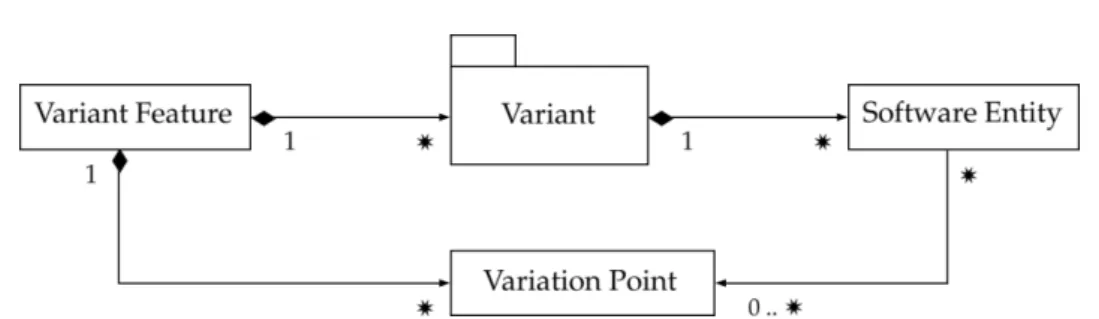
Figure 2.5: The relation between the concepts of feature, variation point with vari-ants and software entities (borrowed fromSvahnberg et al.[2005])

2003] or general for all core assets [e.g., Bachmann et al., 2003; Pohl et al., 2005; Sinnema et al.,2004b].

Further, several approaches for variability management provide detailed re-lationship or mapping models between the variability of core assets at dif-ferent abstraction levels. Mostly, they came in form of a general mapping model [Becker, 2003a,b], metadata model [de Oliveira Junior et al., 2005], basic traceability model [Mohan,2003], a representation independent variability meta-model [Schmid and John, 2003, 2004], a conceptual model for traceability [Berg et al.,2005], or a framework for variability modeling and management in all ab-straction levels [Ch. 9Capilla et al.,2013;Sinnema et al.,2004b]. A common as-pect of these approaches is a formal specification of the relations or associations between the variation points with variants, as variability abstractions in different core assets, the specified variability (e.g., features in an FM), and core assets them-selves. For example, inFigure 2.5we show a simple mapping model between the variant features, variation points with variants in core assets and their relationship with the software entities, without specifying the type of core assets (e.g., require-ments, architecture, code, etc.).

Besides these variability management approaches, there are other approaches that address specifically the variability traceability. Mostly, they address the gen-eral issues of variability traceability management in SPL engineering. For exam-ple, AMPLE [Anquetil et al., 2010] is a general framework based on a reference meta-model for tracing the variability of different types of artifacts by several types of trace links. It discusses the main traceability dimensions in an SPL engineering, specifically when model-driven engineering and aspect-orientation are applied. Quite similarly, XTraQue [Jirapanthong and Zisman, 2009] and the approach by Bayer and Widen[2001] target tracing the variability in different types of artifacts. But, the main idea in XTraQue is to translate the product line documents, the UML documents, into XML documents and to trace their variability by using several types of trace links. So, their main focus is in establishing, using, and/or managing the trace links, without much focus on how the variability in different abstraction levels, or types of core assets, is realized or identified and modeled. They consider that the variability in core assets is already made explicit in someway and need just to be traced.