HAL Id: hal-01834244
https://hal.archives-ouvertes.fr/hal-01834244
Submitted on 10 Jul 2018
HAL is a multi-disciplinary open access
archive for the deposit and dissemination of
sci-entific research documents, whether they are
pub-lished or not. The documents may come from
teaching and research institutions in France or
abroad, or from public or private research centers.
L’archive ouverte pluridisciplinaire HAL, est
destinée au dépôt et à la diffusion de documents
scientifiques de niveau recherche, publiés ou non,
émanant des établissements d’enseignement et de
recherche français ou étrangers, des laboratoires
publics ou privés.
Enhancement of mixing by rodlike polymers
Stefano Musacchio, Dario Vincenzi, Massimo Cencini, Emmanuel Plan
To cite this version:
Stefano Musacchio, Dario Vincenzi, Massimo Cencini, Emmanuel Plan. Enhancement of mixing by
rodlike polymers. European Physical Journal E: Soft matter and biological physics, EDP Sciences:
EPJ, 2018, 41 (7). �hal-01834244�
Stefano Musacchio and Dario Vincenzi Universit´e Cˆote d’Azur, CNRS, LJAD, Nice, France
Massimo Cencini
Istituto dei Sistemi Complessi, CNR, via dei Taurini 19, 00185 Roma, Italy and INFN, Sezione di Roma Tor Vergata,
via della Ricerca Scientifica 1, 00133 Roma, Italy.
Emmanuel L.C. VI M. Plan
Rudolf Peierls Centre for Theoretical Physics, University of Oxford,Oxford OX1 3PU, UK
We study the mixing of a passive scalar field dispersed in a solution of rodlike polymers in two dimensions, by means of numerical simulations of a rheological model for the polymer solution. The flow is driven by a parallel sinusoidal force (Kolmogorov flow). Although the Reynolds number is lower than the critical value for inertial instabilities, the rotational dynamics of the polymers generates a chaotic flow similar to the so-called elastic-turbulence regime observed in extensible polymer solutions. The temporal decay of the variance of the scalar field and its gradients shows that this chaotic flow strongly enhances mixing.
I. INTRODUCTION
The mixing properties of laminar flows are generally poor. In microfluidic applications, where the Reynolds numbers are typically very low, various methods have been developed to enhance the mixing efficiency of the flow. These include the design of grooved walls, the in-troduction of obstacles, the use of a local forcing, or the addition of extensible polymers (e.g., Ref. [1]). In this latter case, elastic stresses can generate instabilities at vanishing fluid inertia that in turn lead to a chaotic flow known as elastic turbulence [2, 3]. It was shown in Ref. [4] that a regime with features similar to those of elastic turbulence can also be obtained via the addition of rigid rodlike polymers, i.e. polymer stretching is not essential for the generation of a chaotic flow at small Reynolds numbers.
The system considered in Ref. [4] is a dilute solution of rodlike polymers driven by a sinusoidal parallel body force (the Kolmogorov force) at a Reynolds number lower than the critical value for inertial hydrodynamic insta-bilities. A similar setting was used previously to study elastic turbulence induced by extensible polymer solu-tions [5]. For low rodlike polymer concentrasolu-tions, the flow is laminar and only displays small deviations from the Newtonian regime. However, when the concentra-tion is increased beyond a critical value, the flow becomes chaotic, the streamlines oscillate and thin vorticity fila-ments form. An inspection of the snapshots of the vor-ticity and polymer-orientation fields show that perturba-tions in the flow are associated with strong deviaperturba-tions of the polymer orientation from the mean-flow direction. The kinetic energy fluctuates around a stationary value lower than that of the laminar case and the mean power required to maintain the mean flow grows with the con-centration, which signals a corresponding increase of the kinetic-energy dissipation. In this regime, the Reynolds
stress is negligible compared to the polymer and viscous ones. In particular, the polymer stress increases as a function of polymer concentration. Thus, the chaotic dy-namics is entirely due to the rotation of polymers, while fluid inertia plays no role. This is further confirmed by the analyis of the kinetic-energy balance in Fourier space. The nonlinear coupling between different Fourier modes due to inertia is indeed negligible; the dynamics of the flow rather results from a scale-by-scale balance between polymer transfer and viscous dissipation. Finally, the kinetic-energy spectrum displays a power law k−α with α 6 3, where k is the wave number. A large number of Fourier modes are thus excited, but the energy is concen-trated on the large scales and fluctuations decay rapidly with the wave number. It should be noted that the ex-ponent α is not universal, since it depends on polymer concentration and the details of the forcing.
Even though the chaotic regime described above is not generated by polymer stretching, it is similar to elastic turbulence in solutions of extensible polymers. The goal of this paper is to show that the addition of rodlike poly-mers can be effectively used to enhance mixing at small Reynolds numbers.
II. PASSIVE-SCALAR DISPERSION IN A SOLUTION OF RODLIKE POLYMERS
The mixing efficiency of a flow can be quantified by studying its ability to disperse a passive scalar field, such as a colorant injected in the fluid.
We consider a scalar field θ(x, t) with diffusivity D in a two-dimensional solution of rodlike polymers. The dy-namics of θ is ruled by the advection–diffusion equation
∂tθ + u · ∇θ = D∆θ , (1)
2
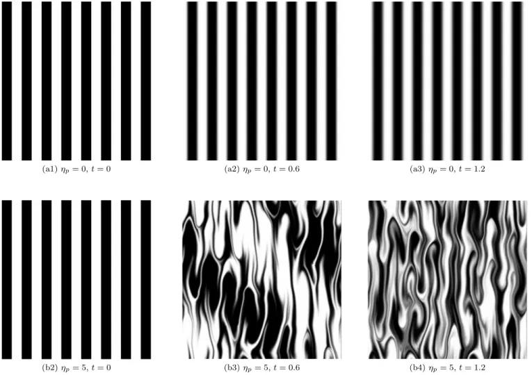
(a1) ηp= 0, t = 0 (a2) ηp= 0, t = 0.6 (a3) ηp= 0, t = 1.2
(b2) ηp= 5, t = 0 (b3) ηp= 5, t = 0.6 (b4) ηp= 5, t = 1.2
FIG. 1: Snapshots of the passive scalar field θ(x, t) at t = 0, 0.6, 1.2 (from left to right) for ηp= 0 (top) and ηp= 5
(bottom) and initial condition B. Here Pe = 1000.
solution. The polymer phase is described by the unit-trace symmetric tensor field R(x, t), the first eigenvector of which yields the average orientation of polymers in a volume element centred at x at time t. In Doi and Ed-wards’ decoupling approximation the fluid and polymer phases evolve according to the following equations [6]:
∂tu + u · ∇u = −∇p + (ν + νp)∆u (2)
+6νηp∇ · [(∇u : R)R] + f ,
∂tR + u · ∇R = (∇u)R + R(∇u)> (3)
−2(∇u : R)R − 2α(2R − I), where (∇u)ij = ∂ui/∂xj, p is pressure, ν is the kinematic
viscosity of the solvent, I is the identity matrix, and νp
and α are proportional to the orientational diffusivity of polymers. In numerical simulations a diffusive term κ∆R (we used κ = 3 × 10⁻³) is added to Eq. (3) in order to improve stability [7]. The parameter ηp determines the
coupling between the polymer phase and the fluid and is an increasing function of the polymer concentration. The values of ηp considered here (ηp 6 5) correspond
to a dilute solution [4, 8]. The above polymer model was studied extensively in the turbulent-drag-reduction regime at high Reynolds number [9].
The system is driven by the Kolmogorov force f (x) = (0, F sin(Kx)), where F and K are the amplitude and the wave number of the force, respectively. In the New-tonian case (ηp = 0), the Navier–Stokes equations
ad-mit the laminar solution u(x) = (0, U0sin(Kx)) with
U0 = F/νK2. This solution is stable if the Reynolds
number Re = U0/νK is smaller than the critical value
Rec =
√
2 (e.g., Ref. [10]). In the following, we take Re = 1 < Rec in order to ensure that inertial effects are
negligible and that the chaotic regime arises solely from the rotational dynamics of the rodlike polymers.
Equations (1), (2) and (3) are solved on a 2π × 2π- do-main periodic in both directions by using a 1/2-dealiased pseudospectral method on a grid with 10242mesh points.
Time integration is performed via a fourth-order Runge– Kutta scheme. In the numerical simulations presented below, we use K = 8, F = 512 and ν = 1. The molec-ular diffusivity is D = 10−3 for most of the simulations
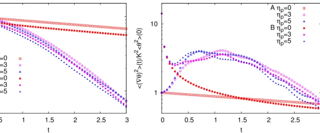
0.1 1 0 0.5 1 1.5 2 2.5 3 < θ 2 >(t)/< θ 2 >(0) t A ηp=0 ηp=3 ηp=5 B ηp=0 ηp=3 ηp=5
FIG. 2: Temporal decay of the variance hθ2i(t),
normalized with its initial value at t = 0, for ηp= 0
(squares), ηp= 3 (circles), ηp= 5 (triangles), and for
initial conditions A (empty symbols) and B (filled symbols). Here Pe = 1000.
reported in Sect. III. The corresponding P´eclet number Pe = U0/KD is Pe = 1000. For the study of the P´eclet
number effects we also consider D = 5×10⁻⁴(Pe = 2000) and D = 2.5 × 10⁻⁴ (Pe = 4000). In addition, the ori-entational diffusion of polymers is disregarded (i.e., we take νp = 0 and α = 0) for two reasons: 1) it is
ex-pected to play a minor role in the chaotic regime and 2) we wish to ensure that the chaotic regime is not triggered by Brownian fluctuations.
In the Newtonian case (ηp = 0), the dynamics of the
velocity field is independent of R and the laminar solu-tion is stable at Re = 1. Therefore we simply integrate Eq. (1) with u(x) = (0, U0sin(Kx)). Conversely, in the
non-Newtonian case (ηp > 0), we performed a
prelimi-nary set of simulations by integrating Eqs. (2) and (3) with initial condition for the velocity field obtained as a small perturbation of the Newtonian stable flow and with the components of R initially distributed randomly. Once the flow has reached the statistically stationary chaotic regime, we start to integrate the dynamics of the scalar field θ.
The initial condition for the scalar field, θ(x, 0), is taken independent of y, so that the initial scalar gradi-ent ∇θ is origradi-ented in the x direction, i.e, perpendicular to the direction of the laminar flow for ηp = 0. This
choice ensures that the mixing in the absence of poly-mers is solely due to molecular diffusion. Two differ-ent initial conditions are considered: A) the monocro-matic function θ(x) = cos(Kx) and B) the step func-tion θ(x) = sign[cos(Kx)]. In both cases we fix K = 8, i.e., the same wavenumber of the base flow. For the former initial condition and in the Newtonian case (ηp = 0), the exponential decay rate of the scalar
vari-ance hθ2i(t) ≡ R θ2(x, t)dx is known analytically as
1 10 0 0.5 1 1.5 2 2.5 3 <( ∇θ ) 2 >(t)/K 2 < θ 2 >(0) t A ηp=0 ηp=3 ηp=5 B ηp=0 ηp=3 ηp=5
FIG. 3: Temporal evolution of the variance of the scalar gradients, h(∇θ)2i(t), for η
p= 0 (squares), ηp= 3
(circles), ηp= 5 (triangles), and for initial conditions A
(empty symbols) and B (filled symbols). Here Pe = 1000.
β0 = −d log[hθ2i(t)]/dt = 2DK2. The latter initial
condition is chosen to mimic the experimental setting in which two differently coloured fluids are injected in a microchannel [3].
III. MIXING ENHANCEMENT
In Figure 1 we compare the temporal evolution of the scalar field with and without polymers starting from the initial condition B. In the absence of polymers, molecular diffusion simply blurs the borders between the white and black stripes, and even after a long time the scalar field remains essentially unmixed. Conversely, over a compa-rable time interval the chaotic flow induced by the rodlike polymers mixes the scalar field efficiently.
To quantify the gain in mixing efficiency, we study the temporal behaviour of the variance of the scalar field and of its gradients. As shown in Fig 2, after an ini-tial transient, the decay rate of hθ2i becomes
indepen-dent of the specific choice of the initial condition. In the Newtonian case, we recover the analytical prediction hθ2i(t) ∝ exp(−β
0t). For ηp > 0, we find that the decay
is much faster. The similar decay observed for the cases ηp= 3 and ηp= 5 suggests a weak dependence of the
de-cay rate on the concentration of polymers. In Ref. [4], it was found that increasing ηpat fixed forcing amplitude F
the resulting chaotic flow displays stronger fluctuations, but the amplitude of the mean flow (which remains si-nusoidal) is reduced. Likely, the combined effect of the reduction of the mean flow and the growth of the fluctu-ations, results in a comparable mixing efficiency for the two cases considered here.
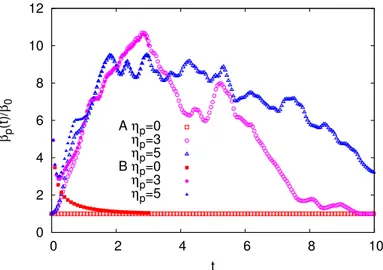
4 0 2 4 6 8 10 12 0 2 4 6 8 10 βp (t)/ β0 t A ηp=0 ηp=3 ηp=5 B ηp=0 ηp=3 ηp=5
FIG. 4: Instantaneous exponential decay rate βp(t),
normalized with β0= 2DK2, for ηp= 0 (squares),
ηp= 3 (circles), ηp= 5 (triangles), and for initial
conditions A (empty symbols) and B (filled symbols). Here Pe = 1000.
the scalar gradients. In the absence of polymers, h(∇θ)2i
asymptotically decays with the same rate as the vari-ance of the field. At short times, however, the decay of h(∇θ)2i depends on the initial condition (Fig. 3). In case
A, which is monochromatic, the decay is purely exponen-tial from the beginning, whereas in case B the decay is faster, since each Fourier mode k of the scalar field decays with a different exponential rate −2Dk2. In the presence
of polymers and in case A, h(∇θ)2i initially grows because mixing creates thin scalar filaments (the so-called direct cascade of passive scalars); at later times when the gra-dient scale reaches the diffusive scale we observe a rapid decay, with a rate similar to that of hθ2i, which indicates
the increased mixing efficiency of the polymer solution with respect to the Newtonian fluid. Case B is similar to case A, except for an initial transient characterized by the fast diffusive decay of the high Fourier modes of the initial condition.
To accurately measure the asymptotic decay of the scalar variance, it is useful to introduce the instantaneous exponential decay rate
βp(t) = − d dtloghθ 2i = β 0 h(∇θ)2i K2hθ2i. (4)
The ratio βp(t)/β0 quantifies the increase of the mixing
efficiency due to the addition of polymers with respect to molecular diffusion only. As shown in Fig 4, the two initial conditions A and B recover the same values of βp(t)
after an initial transient. For ηp= 3 we observe initially a
rapid increase of βp(t), which reaches values much larger
than β0. However, at long times, when the scalar field
is almost completely homogeneized, βp(t) reduces and
eventually returns close to β0. For ηp = 5, after an initial
growth similar to the ηp= 3 case, βp(t) seems to fluctuate
around a constant mean value β∗ in the time interval
t ∈ [2, 4]. At later times βp(t) decreases, but its decay is
slower than for ηp= 3.
We notice that an exponential decay of the passive scalar variance with a constant rate βp(t) implies that
h(∇θ)2i must become proportional to hθ2i, meaning that
the typical scale of the scalar gradients, defined as ` = [hθ2i/h(∇θ)2i]1/2, remains constant. For η
p= 5 we have
that the scale separation between the large scale of the base flow Lu= 2π/K and ` is Lu/` ' 3 for t ∈ [2, 4].
Theoretical predictions on the asymptotic decay of the scalar field have been derived by exploiting the relation between the statistics of Lagrangian trajectories and the statistics of the passive scalar [11, 12]. In particular, it has been shown that for smooth, statistically homoge-neous and isotropic flows, in the limit Pe → ∞ and for large times, the moments of the passive scalar decay ex-ponentially as h|θ|ni ∝ exp(−γnt), with γn linked to the
stretching rate statistics. In our notation βpcorresponds
to γ2. The fact that we observe an exponential decay
with constant βp only for intermediate times could be
due to various causes. The mechanism for the exponen-tial decay [11] originates from the chaotic stretching of the passive scalar, which is effective when there is a large scale separation between the typical scale of the flow Lu
and the diffusive scale (i.e., in the limit Pe → ∞). In the following we will show that the asymptotic decrease of βp(t) observed in Fig 4 could be related to the finite
values of D required by the numerical simulations. Fur-ther, the Kolmogorov flow is neither homogeneous nor isotropic. Moreover, in our case the characteristic large scale of the passive scalar Lθ = 2π/K is equal to that
of the base flow Lu. When Lθ ∼ Lu it has been shown
that the decay, though still exponential, is dominated by “strange eigenmodes” of the advection-diffusion opera-tor [13], and its connection to the Lagrangian stretching rate becomes more complex [12].
On the basis of the previous observations, we ex-pect that the gain in mixing efficiency due to the ad-dition of polymers should depend on the P´eclet number Pe = U0/KD. Increasing Pe at fixed Re reduces β0 but
increases the generation of smaller scales in the scalar field, thus leading to higher values of h(∇θ)2i.
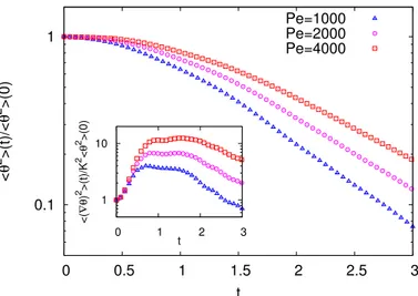
In order to investigate the dependence on Pe, we have compared three simulations with initial condition A at ηp= 5 and Re = 1 with different diffusivities: D = 10−3
(Pe = 1000) D = 5 × 10⁻⁴ (Pe = 2000) and D = 2.5 × 10⁻⁴(Pe = 4000). The decay of the variance for the three cases is shown in Fig. 5. Although an increase of h(∇θ)2i
is observed as a function of Pe at all times (see inset of Fig. 5), the decay of hθ2i is slower at greater Pe because
β0 is reduced. Nevertheless, Fig. 6 shows that the gain
in the mixing efficiency increases with Pe. A power-law fit of β∗, obtained by averaging βp(t)/β0 in the interval
2.5 < t < 4, indicates a growth proportional to Pe0.8. At present we do not have a clear understanding of this power law dependence. We notice that at increasing Pe, the regime in which βp(t) is almost constant continues
0.1 1 0 0.5 1 1.5 2 2.5 3 < θ 2 >(t)/< θ 2 >(0) t Pe=1000 Pe=2000 Pe=4000 1 10 0 1 2 3 <( ∇θ ) 2>(t)/K 2< θ 2>(0) t
FIG. 5: Temporal evolution of the variance hθ2i(t) for
P e = 1000 (triangles), P e = 2000 (circles) and P e = 4000 (squares). Here ηp= 5 and the initial
condition is monochromatic (case A). Inset: Temporal evolution of the variance of the scalar gradients
h(∇θ)2i(t). 1 10 0 2 4 6 8 10 βp (t)/ β0 t Pe=1000 Pe=2000 Pe=4000 10 1000 β* / β0 Pe
FIG. 6: Instantaneous exponential decay rate βp(t),
normalized with β0= 2DK2, for Pe = 1000 (triangles),
Pe = 2000 (circles) and Pe = 4000 (squares). Here ηp= 5 and the initial condition is monochromatic (case
A). Inset: Average exponential decay rate β∗ as a
function of Pe (circles). The line represents the scaling P e0.8.
for longer times. This suggests that the asympotic decay of βp(t) might be a finite-Pe effect.
IV. CONCLUSIONS
The addition of rodlike polymers to a low-Reynolds-number Newtonian fluid generates a chaotic flow, simi-larly to the elastic turbulence regime observed in extensi-ble polymers solutions. We have shown that this regime strongly enhances the mixing of a passive scalar dispersed in the solution. In particular, the variance of the scalar field and of its gradients decays much faster than in the purely diffusive case. Moreover, we found that this effect increases with the P´eclet number. In order to quantify the gain in the mixing efficiency we introduced the instan-taneous exponential decay rate βp(t). The rapid initial
growth of βp(t) to values much higer than the diffusive
decay rate β0provides a precise measure of the increased
mixing. Our results also show that for high P´eclet num-ber and high polymer concentrations, the decay of the scalar variance displays an almost exponential regime, in which βp(t) fluctuates around a constant mean value.
Although our study is conducted in an idealized set-ting, we hope that it can motivate experimental investi-gations of the gain in mixing efficiency obtained via the addition of rodlike polymers to a Newtonian fluid at low Reynolds number. In future investigations it would also be interesting to compare the gain in the mixing efficiency obtained with rodlike or extensible polymer solutions at similar concentrations.
V. ACKNOWLEDGMENTS
The authors acknowledge the support of the EU COST Action MP 1305 “Flowing Matter”. M.C. was partially supported by Universit´e Cˆote d’Azur through Investisse-ments d’Avenir UCA ref. ANR-15-IDEX-01.
VI. AUTHOR CONTRIBUTION STATEMENT
All the authors were involved in the preparation of the manuscript. All the authors have read and approved the final manuscript.
[1] T.M. Squires, S.R. Quake, Rev. Mod. Phys. 77, 977 (2005).
[2] A. Groisman, V. Steinberg, Nature 405, 53 (2000). [3] A. Groisman, V. Steinberg, Nature 410, 905 (2001). [4] E.L.C. VI M. Plan, S. Musacchio, D. Vincenzi, Phys.
Rev. E 96, 053108 (2017).
[5] S. Berti, A. Bistagnino, G. Boffetta, A. Celani, and S. Musacchio. Phys. Rev. E 77, 055306 (2008).
[6] M. Doi, S.F. Edwards, The Theory of Polymer Dynamics (Oxford University Press, Oxford, 1988).
[7] R. Sureshkumar, A.N. Beris, J. Non-Newtonian Fluid Mech. 60, 53 (1995).
6
[8] Y. Amarouchene, D. Bonn, H. Kellay, T.S. Lo, V.S. L’vov, I. Procaccia, Phys. Fluids 20, 065108 (2008). [9] I. Procaccia, V.S. L’vov, R. Benzi, Rev. Mod. Phys. 80,
225 (2008).
[10] S. Musacchio, G. Boffetta, Phys. Rev. E 89, 023004 (2014).
[11] E. Balkovsky, A. Fouxon, Phys, Rev. E 60, 4164 (1999). [12] P.H. Haynes, J. Vanneste, Phys. Fluids 17, 097103
(2005).
[13] J. Sukhatme, R.T. Pierrehumbert, Phys. Rev. E 66, 056302 (2002).