HAL Id: halshs-01109655
https://halshs.archives-ouvertes.fr/halshs-01109655
Submitted on 26 Jan 2015
HAL is a multi-disciplinary open access archive for the deposit and dissemination of sci-entific research documents, whether they are pub-lished or not. The documents may come from
L’archive ouverte pluridisciplinaire HAL, est destinée au dépôt et à la diffusion de documents scientifiques de niveau recherche, publiés ou non, émanant des établissements d’enseignement et de
Ambiguity Preferences and Portfolio Choices: Evidence
from the Field
Milo Bianchi, Jean-Marc Tallon
To cite this version:
Milo Bianchi, Jean-Marc Tallon. Ambiguity Preferences and Portfolio Choices: Evidence from the Field. 2014. �halshs-01109655�
Documents de Travail du
Centre d’Economie de la Sorbonne
Ambiguity Preferences and Portfolio Choices:
Evidence from the Field
Milo B
IANCHI,Jean-Marc T
ALLON2014.65
Ambiguity Preferences and Portfolio Choices:
Evidence from the Field
Milo Bianchiy Jean-Marc Tallonz
September 2, 2014
Abstract
We investigate the empirical relation between ambiguity aversion, risk aversion and portfolio choices. We match administrative panel data on portfolio choices with survey data on preferences over ambi-guity and risk. We report three main …ndings. First, conditional on participation, ambiguity averse investors hold riskier portfolios. Sec-ond, they rebalance their portfolio in a contrarian direction relative to the market. Accordingly, their exposure to risk is more stable over time. Third, their portfolios experience higher returns, but they are also more sensitive to market trends. In several instances, the e¤ects of ambiguity aversion stand in sharp contrast with those of risk aversion.
We thank Roy Kouwenberg, David Schroeder, Paul Smeets, Vassili Vergopoulos, Peter Wakker, seminar participants at Cergy, Stockholm, Toulouse and FUR2014 for very useful comments, and Henri Luomaranta for excellent research assistance. Financial support from AXA Research Fund and from the Risk Foundation (Groupama Chair) is gratefully acknowledged.
yToulouse School of Economics. E-mail: milo.bianchi@tse-fr.eu
1
Introduction
Households have to take more and more complex …nancial decisions, whose consequences are often di¢ cult to predict (Ryan, Trumbull and Tufano (2011), Guiso and Sodini (2012)). Faced with such large uncertainty, house-holds may not behave according to traditional expected utility theory. A large body of literature has developed alternative models of decision mak-ing centered on ambiguity -that is, in Knight (1921)’s words, unmeasurable uncertainty- as opposed to risk -that is, measurable uncertainty. Ambigu-ity has been proposed as a key element for explaining households’…nancial decisions and the functioning of …nancial markets, also in relation to recent …nancial crises.1
This paper provides …eld evidence on the relation between ambiguity aversion and portfolio choices. While several laboratory experiments doc-ument the e¤ects of ambiguity aversion, evidence from the …eld is much scarcer.2 We exploit a unique data set in which administrative panel data on portfolio choices are matched with survey data on preferences over ambi-guity and risk. Our aim is to document whether ambiambi-guity aversion a¤ects portfolio choices and whether this e¤ect may di¤er, even qualitatively, from the one of risk aversion.
We focus on three fundamental aspects of portfolio choices: how much risk households take; how their risk exposure evolves over time through portfolio rebalancing (or lack thereof); and what is the performance of their portfolio. These aspects relate to some of the most important themes in the theoretical literature on portfolio choices under ambiguity. This litera-ture provides (sometimes con‡icting) testable predictions and suggests how portfolio choices may respond di¤erently to attitudes towards ambiguity vs. risk.
Regarding risk taking, ambiguity aversion has been shown to limit par-ticipation in the stock market (Dow and Werlang (1992)). Conditional on participation, however, the relation between ambiguity aversion and risk taking could be positive or negative.3 As for rebalancing, a recent litera-ture shows that ambiguity aversion may lead to forms of portfolio inertia
1
Some contributions on ambiguity and …nancial choices are discussed below. Epstein and Schneider (2010) and Guidolin and Rinaldi (2013) provide recent insightful reviews. On the role of ambiguity in …nancial crises, see e.g. Caballero and Krishnamurthy (2008) and Caballero and Simsek (2013).
2
For a broad survey of the experimental literature on ambiguity aversion, see Traut-mann and Van De Kuilen (2013). In particular, Ahn, Choi, Gale and Kariv (2007) study how ambiguity aversion a¤ects portfolio choices and Bossaerts, Ghirardato, Guarnaschelli and Zame (2010) focus on its e¤ects on asset prices. Later, we review some recent contri-butions drawing from …eld data.
3
Uppal and Wang (2003) provide a model in which ambiguity aversion reinforces risk aversion; Klibano¤, Marinacci and Mukerji (2005) and Gollier (2011) report examples in which ambiguity aversion may increase risk taking.
in that households need not respond to news or to shocks to risk premia.4 Inertia a¤ects the amount of information revealed by prices, as well as their level and volatility (Condie and Ganguli (2012)). Finally, alternative models have been proposed in which ambiguity aversion can either reduce or im-prove portfolio performance.5 Understanding performance is also important
for the debate on the long run survival of ambiguity averse investors (see e.g. Condie (2008) and Guerdijkova and Sciubba (2012)).
In order to guide our empirical investigation, and organize some of these insights in a uni…ed framework, we …rst develop a simple portfolio choice model with a riskless and a risky asset. Building on Epstein and Schnei-der (2010), we assume that both returns and variance of the risky asset are ambiguous: Investors know that higher returns are associated with higher variance, but they do not know the exact form of the trade-o¤. In line with some of the themes already outlined, we derive the following predictions. First, ambiguity averse investors are less likely to invest in the uncertain asset. At the same time, conditional on participation, ambiguity aversion may lead to higher risk taking in that it may induce investors to "underes-timate" the variance of the returns. Third, ambiguity averse investors may be insensitive to small changes in risk premia and so their portfolios may display lower ‡uctuations over time.
Our empirical analysis is based on portfolio data obtained from a large insurance company in France. They focus on a popular investment product among French households dubbed assurance vie. In this product, households decide how to allocate their wealth between relatively safe vs. relatively risky assets, and they can freely change their allocation over time. Our data record the value and detailed composition of the clients’ portfolio of contracts at a monthly frequency for about eight years. Moreover, for each contract, we can construct the corresponding market returns (using Datastream).
Clients were also asked to answer (online while on the phone with a sur-veyor) a survey that we have designed. The survey has two main purposes. First, while portfolio data only concern households’ activities within the company, in the survey we gather a more complete picture of households’ portfolios as well as of various socio-demographic data. Second, we elicit households’preferences over risk and ambiguity.
Following standard procedures, we build our main measure of risk aver-sion by asking subjects to choose between risky vs. safe lotteries. For ambiguity aversion, we ask subjects to choose between risky vs. ambigu-ous lotteries, that is between lotteries with known vs. unknown probability
4
See e.g. Garlappi, Uppal and Wang (2007), Illeditsch (2011), Ganguli, Condie and Illeditsch (2012).
5
In Uppal and Wang (2003) and Boyle, Garlappi, Uppal and Wang (2012), for exam-ple, ambiguity aversion may lead to under diversi…cation and so reduce performance. In Garlappi et al. (2007), instead, ambiguity averse investors may experience higher perfor-mances.
distributions over the …nal payo¤s. These lotteries were hypothetical and involved both gains and losses.6
We start by investigating static portfolio choices. We …nd only weak evidence that ambiguity aversion reduces the probability to hold assurance vie contracts containing risky assets (a form of participation in the stock market). At the same time, however, we …nd that conditional on participa-tion ambiguity averse individuals tend to take more risk. Their contracts are 11% more likely to contain risky assets in a proportion exceeding the median in the sample. Put di¤erently, their contracts display a 7% higher share of wealth invested in risky assets (relative to an average of 56%). This e¤ect is robust as we employ alternative measures of risk taking. As in our model, ambiguity aversion may induce higher risk taking and so have a clearly distinct e¤ect from that of risk aversion.
We then turn to the dynamics of households’ portfolios. In particular, we focus on how households’ exposure to risk, as measured by the share of risky assets in their portfolios, evolves over time. Using each contract’s market returns, we can also distinguish changes in risk exposure which are driven by di¤erential market returns of risky vs. riskless assets from those which result from an active choice of the household (as in Calvet, Campbell and Sodini (2009)).
We show that ambiguity averse investors tend to keep their risk exposure relatively constant over time. Their contracts are 7% less likely to experience monthly ‡uctuations which exceed the median in the sample. Moreover, they tend to rebalance their portfolio in a contrarian direction relative to the market. Speci…cally, ambiguity averse individuals are about 2% less likely to chase returns (that is, to move wealth from assets which have performed relatively poorly to assets which have performed relatively well in their portfolios), relative to an average of 43%. These results are una¤ected by the inclusion of measures of market experiences (such as trends in own portfolio returns) which may a¤ect households’expectations.
Our third set of results concern the performance of these portfolios. We …nd no evidence that ambiguity aversion induces suboptimal portfo-lio choices. Instead, ambiguity averse investors experience about 0:014% higher returns per month (relative to an average of 0:36%). The di¤erence remains signi…cant if we control for the riskiness of the contract, and it be-comes larger if we restrict to risky contracts. At the same time, conditional on risk taking, their returns are more exposed to market trends. In particu-lar, relative to ambiguity neutral investors, their monthly returns are 0:2% higher in good times and 0:13% lower in bad times.
Finally, we perform some robustness checks. We investigate whether our
6We have also elicited preferences through other questions, and the consistency of
the various measures turned out to be good. Moreover, we …nd no strong (if anything, negative) correlation between ambiguity aversion and risk aversion, which suggests that the two variables re‡ect di¤erent individual traits. We refer to Section 3 for details.
estimates may be driven by omitted behavioral characteristics, and show that the e¤ects of ambiguity aversion are robust to the inclusion of measures of investors’sophistication, con…dence, and time preferences. We also shed some light on whether our …ndings appear representative of households’ behaviors in their broader portfolio. We show that our results hold (they are sometimes stronger) for clients with a large fraction of wealth invested in the company, for which the observed portfolio is probably more representative of the overall portfolio.
In the next sections, we further discuss each of these …ndings as well as their relation with the existing literature. Already at this stage, however, we wish to highlight some of their implications from a somewhat broader perspective. First, our results show that measures of preferences as elicited in surveys can be informative about choices made in the real world. We …nd it remarkable that these measures show some predictive power in a context like portfolio choices in which heterogeneity is large and often di¢ cult to explain with standard observables.
Moreover, we believe that our results are strongly suggestive that ambi-guity and risk are fundamentally distinct objects, not only conceptually but also from an empirical viewpoint. In several instances, ambiguity aversion displays opposite e¤ects than risk aversion. In our view, this provides sup-port to the view that ambiguity aversion cannot be reduced to an additional source of aversion to risk.
The paper proceeds as follows. In the next subsection, we review our contribution in relation to the existing literature. A model is provided in Section 2. In Section 3, we present the data. In Section 4, we describe our method for eliciting ambiguity and risk preferences and provide some descriptive statistics on their determinants. Our main results on portfolio choices appear in Section 5. In Section 6, we discuss robustness checks. We conclude in Section 7. A detailed description of our variables, …gures and tables are in the Appendix.
1.1 Literature
To our knowledge, this study is the …rst to provide evidence on the e¤ect of ambiguity aversion on …nancial decisions as observed in administrative data. As such, it contributes to two streams of literature. First, we relate to the household …nance literature by looking at the determinants of house-holds’…nancial decisions. The literature is growing rapidly and we refer to Campbell (2006) and Guiso and Sodini (2012) for excellent recent surveys. Compared to this literature, our main novelty is in matching survey and administrative data. While as pointed out this does not provide a detailed picture of the entire households’portfolios (as for example in Calvet, Camp-bell and Sodini (2007) and Calvet et al. (2009)), it o¤ers the opportunity to study the relation between behavioral traits and real choices. This seems
to accommodate (some of) the desiderata expressed in Campbell, Jackson, Madrian and Tufano (2011).7
We know of only a few studies combining survey and administrative data. Dorn and Huberman (2005) focus on the relation between risk aversion, (perceived) …nancial sophistication and portfolio choices; Alvarez, Guiso and Lippi (2012) analyze the frequency with which investors observe and trade their portfolio; Guiso, Sapienza and Zingales (2013) and Ho¤mann, Post and Pennings (2013) study how risk aversion has changed following the …nancial crisis; Bauer and Smeets (2014) and Riedl and Smeets (2014) investigate how social preferences a¤ect socially responsible investments. None of these studies focuses on ambiguity preferences as we do.
Second, we contribute to the literature on ambiguity preferences. Models of ambiguity attitudes have ‡ourished over the past two decades and we refer to Etner, Jeleva and Tallon (2012) for a recent review. As already mentioned in the Introduction, while these models have received considerable attention also in relation to …nancial decisions, empirical studies are quite scant.8
Most closely related to our study, Dimmock, Kouwenberg and Wakker (2013) and Dimmock, Kouwenberg, Mitchell and Peijnenburg (2013) exploit large representative surveys in which subjects are asked about their prefer-ences as well as about their portfolio holdings. Dimmock, Kouwenberg and Wakker (2013) …nd no correlation between ambiguity aversion and stock market participation in a Dutch sample. Dimmock, Kouwenberg, Mitchell and Peijnenburg (2013) show that stock market participation as well as the share of the wealth invested in equity are negatively related to ambiguity aversion in the American Life Panel sample.
We share with these authors a similar methodology to elicit ambiguity aversion (but our subjects receive no monetary reward in relation to their choices) and a similar focus on the relation with …nancial choices. Their data are based on surveys, and they are larger in size and in scope. Our administrative data provide more details for the speci…c investment at study as well as a panel structure, which allows us to address di¤erent questions such as portfolio dynamics and performance.
2
Model
We …rst develop a simple model that highlights the various forces at work in portfolio choice under ambiguity. We build on a model presented in
7They report an "urgent need" for household-level …eld data which would provide better
accuracy and granularity than standard surveys and which would be even more useful if matched with survey data on households’beliefs and objectives.
8
Recent developments include Maccheroni, Marinacci and Ru¢ no (2013) on mean-variance preferences; Epstein and Ji (2013) and Lin and Riedel (2014) on dynamic portfolio choices; Collard, Mukerji, Sheppard and Tallon (2012) and Ju and Miao (2012) on the equity premium puzzle.
Epstein and Schneider (2010) in which ambiguity bears both on the mean and the variance of the asset returns. We extend it by considering general CRRA utility functions and introducing an explicit parameterization of the investor’s attitudes towards ambiguity.
Consider an agent who has to allocate her initial wealth W0 among two
assets, one “safe”and one “ambiguous.”She has a utility function over …nal wealth W1 de…ned as
u(W1) =
W11
1 ;
where is the coe¢ cient of constant relative risk aversion. She can choose to hold a fraction of her wealth in the ambiguous asset, and (1 ) in the safe asset. The safe return is denoted Rf and rf = log(1 + Rf).
The ambiguous return is denoted eR, with er = log(1 + eR). The returns are known to be lognormally distributed (with mean r and variance 2) but the investor is uncertain of the “true” distribution. As in Epstein and Schneider (2010), uncertainty is described by a single parameter x; which a¤ects positively both the mean and the variance of the returns. The investor knows that the ambiguous asset can have either low return and low volatility or high return and high volatility, but not the exact values. Speci…cally, mean returns are given by r = r + x and their variance by 2 = 2+ x, where is a known positive parameter and x is an index of the ambiguity on the …nancial markets which takes value in an interval [x; x]:
We assume, in the spirit of Gajdos, Hayashi, Tallon and Vergnaud (2008), that the investor, facing this set of possible laws for the returns, considers that the “central” one, indexed by ^x = (x + x)=2, is more salient. She then wants to insure that her decision is “robust” to other distributions around this central one. Her concern for robustness, which we interpret as her ambiguity attitude, is captured by a parameter 2 [0; 1]. When = 0, she just considers the central scenario and does not care for robustness. When
= 1, she puts all the weight on the worst possible scenario.
Denoting x = x + (1 )^x and x = x + (1 )^x, the maximization problem is thus: max 2[0;1]x2[x ;x ]min Ex f W11 1 ;
s.t. fW1 = ( ( eR Rf) + (1 + Rf))W0. Hence, taking logs and using the
approximation of log returns on wealth developed by Campbell and Viceira (2002), the problem the decision maker has to solve is:
max 2[0;1]x2[x ;x ]min (r + x rf) + 1 2 ( 2+ x) 1 2 2( 2+ x): (1)
For a given x, we can de…ne
?(x) = r + x rf + 1
2( 2+ x)
( 2+ x) ; (2)
that is the optimal share of the ambiguous asset when the return follows a log normal distribution of mean r + x and variance 2+ x. The expression corresponds to the standard mean-variance portfolio with the addition of one-half the variance at the numerator. As shown in Campbell and Viceira (2002), this term converts from log to simple returns. Here, the expected log return and variance include a term in x, which embodies ambiguity.
Notice that in our setting any realization of x has two opposite e¤ects. A low x; for example, carries the good news that volatility is low and at the same time the bad news that mean returns are low. Whether good news or bad news prevail depends on the level of : When considering moderate exposure to risk, that is for < (2 + )= ; the utility of the decision maker is increasing in x and the worst scenario is a low x: According to (1), then, an ambiguity averse agent will optimize against the lower measure indexed by x . Conversely, for positions larger than (2 + )= ; the utility is decreasing in x and the ambiguity averse investor optimizes against the distribution indexed by x .
When = (2 + )= ; the two e¤ects exactly cancel out and the utility does not depend on x. Hence, in this setting, two portfolios can completely shield the decision maker from any ambiguity. First, as usual, the one with no ambiguous asset, = 0: Second, the portfolio with = (2 + )= , at which the trade-o¤ between return and volatility does not depend on the ambiguity on these parameters. Away from these portfolios, the decision maker will bear some ambiguity.
We can then express more precisely how the optimal share ?( ) varies depending on the excess returns r rf. De…ne the cut-o¤ values
r0 = 1 2 2+ x x ; r 1= 1 2 + 2 2 + 1 + 2 x ; r2 = 1 2 + 2 2 + 1 + 2 x ; where for any given we have r0 r1 r2: The optimal demand for the
ambiguous assets is ?( ) = 8 > > < > > : 0 if r rf r0 min( ?(x ); 1) if r0 r rf r1 min(2+ ; 1) if r1 r rf r2 min( ?(x ); 1) if r rf r2:
In Figure 8.2, we illustrate the shape of ?( ) as well as the comparative statics with respect to ambiguity aversion : The demand of an ambiguity neutral investor corresponds to the circled line; an increase in corresponds to the red dotted curve.
There are four regions to be considered. When excess returns are low, the optimal demand is exclusively composed of the safe asset and ?( ) = 0. The non-participation region increases in ambiguity aversion: The larger ambiguity aversion, the higher premium an investor requires in order to invest in the ambiguous asset. This is a well-known e¤ect going back to Dow and Werlang (1992).
When returns are larger than r0, the demand ?( ) is positive and
de-pends on the perceived trade-o¤ between risk and returns; that is, on which “as if” beliefs the investor uses. For relatively low excess return, the in-vestor acts as if the process was governed by x , i.e., low mean return and low volatility. This corresponds to the demand ?(x ):
An important observation is that, for a range of returns (strictly) be-tween r0 and r2, the demand for the risky asset may actually increase in
ambiguity aversion. The reason is that, as mentioned, considering the worst scenario induces to behave as if volatility was low. Hence, in a sense, am-biguity aversion induces investors to "underestimate" volatility and that increases their demand for the risky asset.
The possibility that ambiguity aversion may increase risk taking was al-ready noticed in Klibano¤ et al. (2005) and Gollier (2011). Our mechanism however is somewhat distinct and relies on the fact that ambiguity concerns both mean and variance of returns. We also notice that the region in which
?( ) is higher for the ambiguity averse agent expands with ambiguity
aver-sion.
The third region, r1 r rf r2; corresponds to the case in which
the demand does not vary with the risk premium. This implies a form of portfolio inertia, in that small shocks to risk premia do not a¤ect investors’ demand. Given that as argued a portfolio with = (2 + )= provides complete hedging against ambiguity, it takes a large shock to returns to induce an ambiguity averse investor to change her demand. Notice also that when = 0 (ambiguity neutrality), investors display no inertia and, more generally, the inertia region increases with the degree of ambiguity aversion. Inertia implies that, for more ambiguity averse investors, portfolios do not ‡uctuate much in response to shocks.
The possibility of portfolio inertia even at a non-zero ambiguous position was already shown in Epstein and Schneider (2010) and more generally in Illeditsch (2011). Related forms of portfolio inertia, driven by lack of response to news, appear in Garlappi et al. (2007) and Ganguli et al. (2012). An important observation for our next empirical analysis is that, away from zero, portfolio inertia does not imply absence of rebalancing. On the contrary, it may require to continuously rebalance the portfolio so as to
compensate the ‡uctuations induced by the market. Suppose for example that realized returns of the ambiguous asset exceed risk-free returns; then, the fraction of wealth invested in ambiguous assets would mechanically in-crease. If the investor wishes to keep her risk exposure constant, she needs to reallocate wealth from the ambiguous to the riskless asset.
Finally, in the region where the mean excess return is r rf r2, the
investor acts as if the process is governed by x , i.e., high mean return and high volatility. This leads to the demand ?(x ); which decreases with .
We summarize in the following points, which will serve as a guide for the next empirical analysis.9 According to our model:
(i) Ambiguity aversion increases the non-participation region.
(ii) Conditional on participation, the demand ?( ) may increase or de-crease with ambiguity aversion:
(iii) Ambiguity averse investors are more likely to display portfolio inertia and lower ‡uctuations in their demand.
3
Data
We exploit three sources of data. First, we have obtained administrative data on portfolio choices from a large French insurance company. These data describe the value and the detailed composition of clients’holdings of assurance vie contracts. Despite their name, these are not insurance but investment products.10
Assurance vie contracts are widespread in France, they are the most common way through which households invest in the stock market.11
Ac-cordingly, our sample can be considered broadly representative of French households. For example, the median total wealth in our sample is between 225 and 300 thousand euros and the median …nancial wealth is between 16 and 50 thousands euros. These …gures are in line with those obtained for the general French population (see Arrondel, Borgy and Savignac (2012)).12
9
Notice that our model does not incorporate ambiguity lovers. Our qualitative predic-tions would not be changed by allowing for this possibility.
1 0
The name is due to the fact that, for …scal reasons, the contract is formally structured as an insurance in case of death coupled with an insurance in case of life. A speci…c feature of the product is that there is some incentive not to liquidate the contract before some time (8 years in our sample period) so as to take advantage of reduced taxes on capital gains.
1 1
According to the French National Institute for Statistics, 41% of French households held at least one of these contracts in 2010. This makes it the most widespread …nancial product after Livret A, a saving account whose returns are set by the state. See INSEE Premiere n. 1361 - July 2011 (http://www.insee.fr/fr/¤c/ipweb/ip1361/ip1361.pdf).
1 2
For o¢ cial and comprehensive data, see the 2010 Household
A typical assurance vie contract establishes the types of funds in which the household wishes to invest and the amount of wealth allocated to each fund. A key distinction is between relatively safe vs. relatively risky funds. The …rst assets, which are called euro funds, are basically bundles of bonds. Their returns are rather stable and the capital invested is guaranteed by the company. In the sequel, we will simply refer to those as riskless assets.
The second funds are bundles of stocks, whose returns or capital is not guaranteed. The client can choose in some details the composition of their risky assets. In the sequel, we will simply refer to those as risky assets. Over time, clients are free to change the composition of their portfolios, make new investment and withdraw money as they wish. There are no restrictions in the number of contracts each household can have.
Speci…cally, our data record at a monthly frequency the activities in these contracts from September 2002 to April 2011. The sample includes 511 clients and 1357 contracts.13 These contracts can represent a sizeable fraction of households’…nancial wealth. In our sample, the average value of a contract is 16; 900 euros, the maximum is 340; 000 euros.
Our second source of data concerns market returns. As we have detailed information about the composition of each contract, we can look for the market returns experienced in a given month by each fund contained in the contract. We obtain these returns from Thomson Reuters Datastream and, based on those, we can build the corresponding market returns for each contract.
Our third source of data is a survey we have designed and conducted on these same clients. The survey was administered by a professional com-pany at the end of 2010.14 We have two main purposes. First, we wish to gather information about demographic characteristics, wealth and portfolio holdings outside the company. This helps having a broader picture of the clients’…nancial activities.
Second, we wish to have an idea of clients’ behavioral characteristics, and in particular of their preferences over risk and ambiguity.15 In the next section, we describe how we have elicited these preferences.
(http://www.insee.fr/en/methodes/default.asp?page=sources/ope-enquete-patrimoine.htm).
1 3
In our sample, 65% of the clients hold more than one contract. The median number of contracts by client is 2.
1 4
It was made clear to the subjects that they were contacted as part of a scienti…c project on risk, while the insurance company was never mentioned during the interview. Clients were contacted over the phone and they completed the survey over the internet while in line with the surveyor.
1 5The survey also includes a set of questions on preferences over time, expectations and
sophistication, which are however not the main focus of the present paper. We brie‡y discuss some of them in Section 6.
4
Risk and Ambiguity Preferences
We elicit preferences over risk in a classical way.16 We ask respondents to choose between an hypothetical lottery and a sure outcome. Depending on their answer, we sequentially provide alternative lotteries in which the risky lottery is made relatively more or less attractive.
Speci…cally, we ask: "You have two options: (a) win 400 euros for sure vs. (b) win 1000 euros with 50% chance and zero otherwise. Which one would you choose?" In case (a) is chosen, lottery (a) is replaced by a lottery which o¤ers 300 euros for sure (while the risky lottery remains the same). If instead (b) is chosen, lottery (a) is replaced by a lottery which o¤ers 500 euros for sure. We have also asked very similar questions with lotteries involving losses (see Appendix 8.1 for details).
When lotteries involved gains, 59% of our respondents always chose the riskless lottery (thereby preferring 300 for sure rather than 1000 with 50% chance), 19% chose …rst the risky and then the riskless lottery, 4% chose …rst the riskless and then the risky lottery, and the remaining 18% always chose the risky lottery. When lotteries involved losses, the corresponding proportions were respectively 14%, 23%, 22% and 41%: Consistently with a large literature, we observe that respondents tend to show higher risk aversion over gains than over losses. We also observe a positive correlation between risk aversion over gains and over losses.
These responses can be used to order the respondents in terms of risk aversion. We build an aggregate measure of risk aversion over gains and over losses and we de…ne the dummy Risk Averse as equal to 1 if risk aversion exceeds the median in the sample.
We follow a similar procedure in order to elicit ambiguity preferences.17
We ask to choose between (a) win 1000 euros with a completely unknown probability vs. (b) win 1000 euros with 50% chance and zero otherwise. If (a) is chosen, the risky lottery is replaced by one o¤ering to win 1000 euros with 60% chance. If instead (b) is chosen, the risky lottery is replaced by one o¤ering to win 1000 euros with 40% chance. Also in this case, we have repeated the questions with lotteries involving losses.
When lotteries involved gains, 57% of our respondents always chose the risky lottery (thereby preferring 1000 with 40% chance rather than with an
1 6
Alternatively, risk preferences may be estimated by revealed preferences from the ob-served portfolio choices (together with a set of assumptions on utility functions, beliefs, ...). Approaches along these lines include Cohen and Einav (2007); Barseghyan, Molinari, O’Donoghue and Teitelbaum (2013); Barseghyan, Molinari and Teitelbaum (2014) (see Guiso and Sodini (2012) for a discussion of the various approaches). Exploring the consis-tency of estimates based on survey vs. those based on revealed preferences is in our view a very interesting topic for future research.
1 7
Dimmock, Kouwenberg and Wakker (2013) provide a decision theoretic foundation for this method, showing that ambiguity attitudes can be entirely described by matching probabilities.
unknown probability), 14% chose …rst the risky and then the ambiguous lottery, 15% chose …rst the ambiguous and then the risky lottery, and the remaining 14% always chose the ambiguous lottery. When lotteries involved losses, the corresponding proportions were respectively 37%; 26%, 19%, and 17%: In the same way as for risk, we build an aggregate measure of ambiguity aversion over gains and over losses, and we de…ne the dummy Ambiguity Averse as equal to 1 if ambiguity aversion exceeds the median in the sample. In Appendix 8.1, we provide a more detailed description of these vari-ables, as well as of the other variables used in the subsequent analysis. In Table 1, we report some descriptive statistics. In Table 2, we report the correlation between our measures of ambiguity aversion, risk aversion and a set of demographic characteristics. In column (1), Risk Averse appears negatively related with age and wealth. As for Ambiguity Averse, in column (2), our demographic characteristics seem to have very little explanatory power.
In columns (3)-(4), we see that the relation between Ambiguity Averse and Risk Averse is not very strong and, if anything, it is negative. This is consistent with the evidence reported in Dimmock, Kouwenberg and Wakker (2013).18 Importantly for our purposes, this potentially allows us to distin-guish in our subsequent analysis the e¤ects of ambiguity aversion from that of risk aversion.
As we have elicited risk preferences in other questions as well, we can investigate the consistency of our estimates.19 In column (5), we report the relation between Risk Averse and Job Lottery, in which risk aversion is elicited as in Barsky, Juster, Kimball and Shapiro (1997). The respondent is asked to choose between di¤erent jobs: one granting his/her current revenues forever vs. a riskier job. Depending on the answers, more or less attractive risky jobs are then sequentially o¤ered. The two measures of risk aversion are positively related, and the relation is signi…cant at the 5% level.
In column (6), the variable Certainty Equivalent is based on the will-ingness to pay for a lottery in which a coin is tossed 100 times and 1 euro is obtained each time head occurs (similarly to Mansour, Jouini and Napp (2006)). The relation with Risk Averse is negative as one would expect, even though only marginally signi…cant.
Overall, the various measures give a consistent picture, which is reassur-ing on the validity of our methods for elicitreassur-ing risk preferences.20 We can
1 8The evidence on the relation between risk and ambiguity preference is not abundant,
and it does not give a clear picture. Butler, Guiso and Jappelli (2012) document instead a positive relation between the two.
1 9We have no other quantitative questions eliciting ambiguity preferences.
2 0
Indeed, our results would not be qualitatively di¤erent if we used these alternative measures of risk aversion. We emphasize the variable Risk Averse because it involves risk preferences both over gains and over losses, and because its framing is similar to the one on ambiguity preferences.
then turn to our main purpose of investigating whether these measures have any predictive power on real life portfolio choices.
5
Empirical Analysis
We divide our empirical investigation into three parts. First, we study static portfolio choices. Then, we look at how households rebalance their contracts over time. Last, we study the performance of their portfolios. We will study when and how ambiguity aversion plays a role, in particular compared to risk aversion, in these three important dimensions of portfolio choice.
5.1 Static Portfolio Choices
We start by considering the propensity to hold a risky portfolio; then, we focus on risky contracts and consider the value of risky assets as a fraction of the total portfolio. Holding a risky portfolio may be related to households’ participation in the stock market. As mentioned, starting from Dow and Werlang (1992), it has been shown theoretically that ambiguity aversion may induce households to refrain from investing in stocks.
The value of risky assets as a fraction of the total portfolio is instead a way to account for households’exposure to risk. The measure is simple (and probably most salient to decision makers) and, as in Calvet et al. (2007), it is highly correlated with the actual risk experienced in the portfolio (as measured by the standard deviation or the beta of the returns). Moreover, as suggested in Section 2, the e¤ect of risk vs. ambiguity preferences may be particularly interesting here: While risk aversion should clearly reduce risk taking, the relation with ambiguity aversion is less clear-cut.
Our investigation starts by estimating the following equation:
i;c;t = + 1ambigi+ 2riski+ X
0
i + t+ "i;c;t: (3)
In equation (3), i;c;t denotes the choice of individual i on contract c at
time t, Xi0 includes a set of standard demographic variables (age, gender, education, marital status, income, wealth) and t are month-year …xed-e¤ects. Our coe¢ cient of interest are 1 and 2; which describe respectively the impact of ambiguity and risk preferences, as elicited in our survey, on the portfolio choice. As the choices of a given individual may be correlated across contracts as well as over time, we cluster standard errors at the individual level.21
We …rst report our results on the likelihood to hold risky portfolios.22
2 1
We have also performed our regressions by clustering both at the time and at the individual level, using a method suggested by Petersen (2009). Results are not changed.
2 2
For simplicity, throughout the paper, we report results based on OLS estimates. Re-sults do not change if, for categorical or censored variables, we employ probit or tobit
In our sample, on average 42% of the contracts contain some risky asset. According to our model and to the literature quoted above, this fraction should decrease both with risk and with ambiguity aversion. In columns (1)-(3) of Table 3, the dependent variable is a dummy equal to one if the contract contains some risky asset. It appears that ambiguity aversion decreases the propensity to hold a risky contract, but standard errors are large. The e¤ect of risk aversion too is negative but not signi…cant.
These results are not conclusive. As mentioned, this appears to be the case also in Dimmock, Kouwenberg and Wakker (2013), who report no sig-ni…cant relation between ambiguity aversion and stock market participation on Dutch households. On the other hand, Dimmock, Kouwenberg, Mitchell and Peijnenburg (2013) …nd a negative and signi…cant relation in the Amer-ican Life Panel data. We also notice that, while holding risky assurance vie contracts is a form of participation in the stock market, our evidence on participation is only partial as we lack a detailed picture of households’ entire portfolios. Finally, participation in the stock market via assurance vie contracts is quite widespread (much more than participation via direct stock holdings). In our sample, 75% of clients hold a risky contract at some point in time. This may limit the variation observed across households and so partly explain low statistical power.
We then turn to the e¤ects of ambiguity and risk preferences on the risky share. In columns (4)-(6), the sample is restricted to risky contracts and the dependent variable is a dummy equal to 1 if the value of the risky assets over the total value of the contract exceeds the median in the sample (that is equal to 0:51). The e¤ect of risk aversion does not appear statistically signi…cant. On the other hand, ambiguity aversion is strongly related to risk taking, and the relation is positive. Ambiguity averse individuals are 11% more likely to hold a contract with a large risk exposure (where "large" is de…ned relative to the median in the sample).
In Table 4, we check whether this relation is robust to alternative mea-sures of risk taking. In columns (1)-(2), we show that ambiguity averse in-dividuals hold contracts with a 7% higher share of wealth invested in risky assets (relative to an average share of 56%). A similar picture obtains as we measure risk taking by the standard deviation of the returns (columns 3-4) and by the beta of the portfolio (column 5-6).23 Moreover, unreported results show that the coe¢ cients are not a¤ected by the inclusion (or exclu-sion) of the various controls. Overall, the result appears robust: Conditional on holding risky assets, ambiguity averse individuals tend to take more risk.
models.
2 3The variable Std Dev refers to the standard deviation of the returns in the previous
12 months. The variable Beta is a measure of systematic risk constructed by regressing portfolio returns in the previous 12 months on the French stock market index CAC40.
While somewhat surprising, this result can be accounted for by the model of Section 2 in which the share of the ambiguity asset might increase with ambiguity aversion. This occurs when the “worst scenario”is the low mean, low variance con…guration. The corresponding prior therefore tends to “un-derestimate”the variance relative to the ambiguity neutral prior, which may lead the investor to take more risk. More generally, these results are clearly suggestive that risk and ambiguity preferences need not a¤ect choices in the same way and may actually push in opposite directions.
5.2 Dynamic Portfolio Choices
A distinctive feature of our database is its panel dimension: we observe clients’behavior at a monthly frequency for about 8 years. This allows us to explore how investors change their exposure to risk over time, and so to relate to a recent literature on dynamic portfolio choices under ambiguity aversion. In particular, we can investigate whether ambiguity averse investors exhibit some form of portfolio inertia.
In our model, as in Epstein and Schneider (2010) and more generally in Illeditsch (2011), inertia may occur also when households have a positive exposure to risk, if they have chosen their exposure so as to hedge against ambiguity. In this case, they wish to keep it constant even after (small) shocks to expected returns or perceived uncertainty. Garlappi et al. (2007) ad Ganguli et al. (2012) also show that ambiguity averse investors may not change much their portfolio weights as they tend to ignore news about future returns. Portfolio inertia impacts the amount of information revealed in prices and ultimately their level and volatility (Condie and Ganguli (2012)). We now consider how households’exposure to risk, as measured by the share of risky assets in their portfolios, evolves over time. Following Calvet et al. (2009), we distinguish passive and active changes in risk exposure. The …rst is driven by di¤erential market returns of risky vs. riskless assets: if the former outperform the latter, the risky share tends to increase (and vice-versa). On top of this, investors may change their risk exposure by actively rebalancing their portfolios or investing/withdrawing money from the various assets.
Speci…cally, keeping the notation of Section 2, suppose that ^R Rf is
the realized excess return of the risky asset between t 1 and t: The passive share is de…ned as P t = (1 + ^R) t 1 1 + Rf + ( ^R Rf) t 1 : (4)
If we observe that the risky share moves from t 1to t; we de…ne the passive
change as
and the active change as
ACt= t Pt: (6)
If t 1 2 (0; 1); we can look at the sign of the ratio ACt=P Ct. A
posi-tive ratio indicates that an investor is rebalancing his contract in the same direction as the market; that is, he is investing relatively more in assets which have performed better in the past. We say he acts as a chaser. A negative ratio instead indicates that an investor is rebalancing his portfolio contrary to the market, and we refer to him as contrarian. Notice that a special case of contrarian behavior is de…ned by those individuals who wish to keep their risky share constant over time, and they continuously rebal-ance their portfolio accordingly. For those individuals, we should observe that ACt=P Ct= 1:
Of course, individuals may remain inactive. On average, 64% of the contracts show zero active change in a given month. Restricting to risky contracts, the average is 21%. These …gures provide a lower bound on the fraction of contracts for which there is no active rebalancing in a given month.24
We …rst consider how ambiguity and risk preferences a¤ect the magni-tude of the changes in risk exposure over time. In column (1) of Table 5, the dependent variable is a dummy equal to one if the total change in the risk pro…le j t t 1j exceeds in absolute value the median in the sample
(that is equal to zero). In column (2), we look at relative changes in risk pro…le, that is j( t t 1)= t 1j and so we restrict the sample to contracts
with t 1> 0. We construct a dummy equal to one if the relative change in
the risk pro…le exceeds in absolute value the median in the sample (that is equal to 0:96%).
In both columns, it appears that ambiguity aversion leads to more stable risky shares over time. More precisely, contracts held by ambiguity averse individuals are 7% less likely to experience large ‡uctuations from one month to the next, where "large" is de…ned relative to the median in the sample. The e¤ect of risk aversion is negative but not signi…cant.
In columns (3)-(4), we focus on active changes. In column (3), the de-pendent variable is a dummy equal to one if the active change in the risk pro…le t Pt exceeds in absolute value the median in the sample (that
is equal to zero). In column (4), the dependent variable is a dummy equal to one if the relative active change ( t Pt)= Pt exceeds in absolute value
the median in the sample (that is equal to 0:56%). Consistently with the previous results, we see that ambiguity averse individuals are less likely to actively induce large ‡uctuations in their risk exposure.
We then investigate in more details the direction of rebalancing. In
2 4These are lower bounds since values of active change close to zero may not be due to
small rebalancing but just to measurement error (e.g. driven by rounding o¤ the passive share).
Table 6, the dependent variable is chaser, that is a dummy equal to one if ACt=P Ct > 0 and to zero if ACt=P Ct < 0: From columns (1)-(3), we see
that ambiguity averse individuals are about 2% less likely to chase returns (relative to an average of 43%). The e¤ect of risk aversion is not signi…cant. Portfolio rebalancing depends also on beliefs about future returns, which in turn may be a¤ected by observed returns. Hurd, Van Rooij and Winter (2011) show that recent stock market increases tend to raise the expectation about future market returns. Similarly, Vissing-Jorgensen (2004) documents how households change their expectations in response to their own past returns. Accordingly, we check the robustness of our results to the inclusion of controls on market experiences such as past portfolio returns.25 This is also a way to compare the magnitude of the e¤ects of ambiguity aversion (a behavioral trait) with those of market experiences.
Speci…cally, in column (4), we include a measure of global market trends (instead of time …xed e¤ects). The variable Good Times is a dummy equal to one if the average monthly returns observed in a given month exceed the median returns in our sample (equal to 0:44%). The estimate shows that, in good times investors are 3% more likely to chase returns. The coe¢ cient on ambiguity aversion is not a¤ected.
In column (5), the variable Overperform is a dummy equal to one if the returns of the contract between t 1 and t exceed the median market returns in that month. Individuals who have performed well relative to the market are 4% more likely to chase returns, and again the coe¢ cient on ambiguity aversion remains unchanged.
In columns (6), we consider whether a given contract is experiencing a better trend than the median contract. Speci…cally, the variable Improve is a dummy equal to one if the di¤erence between current and past returns exceeds the market median di¤erence in the same period. The e¤ect is positive and bigger than the previous e¤ects: Individuals who experience better trends are 14% more likely to act as chaser.
In magnitude, the e¤ect of ambiguity aversion appears smaller than the one of market experiences. Still, the estimates are signi…cant and robust across speci…cations. Ambiguity averse investors are less likely to chase returns. This is consistent with our model in that their demand for the risky asset may be ‡at, so small ‡uctuations in risk premia need not generate any change in the demand of these investors. This is also consistent with the evidence of Table 5 whereby ambiguity averse investors show relatively stable risky shares over time.
2 5
Moreover, in Section 6, we consider other behavioral traits which may a¤ect stock market expectations.
5.3 Performance
We now turn to the relation between ambiguity preferences and portfolio returns. Some scholars have proposed models in which ambiguity aver-sion leads to under diversi…cation, that is to a portfolio which is biased to-wards less ambiguous assets (relative to standard mean-variance portfolio).26 Based on these insights, one may expect that ambiguity averse investors ex-perience lower performances in their contracts. On the other hand, Garlappi et al. (2007) have shown that ambiguity averse investors (who are less sensi-tive to information about expected returns) may earn higher out-of-sample Sharpe Ratios when expected returns are di¢ cult to predict.
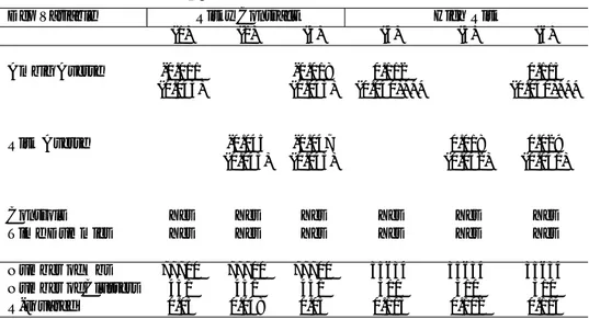
This debate is also relevant for the literature on the long run survival of ambiguity averse investors and so on their aggregate impact on asset prices. Condie (2008) shows that, in markets with aggregate risk and rational utility maximizers, ambiguity averse investors should not be expected to survive. Guerdijkova and Sciubba (2012) provide a model in which ambiguity averse investors may survive despite their distorted beliefs as ambiguity aversion may act as an extra discount factor and so increase the propensity to save. We start by considering the entire sample of contracts. In Table 7, the dependent variable is the monthly return (in percentage points) experienced in a given contract. The average monthly return in the overall sample is 0:36%. Restricting to risky contracts, the average is 0:39%. In column (1), it appears that ambiguity averse individuals experience higher raw returns and risk averse individuals experience lower raw returns. This may just re‡ect the evidence presented earlier that ambiguity averse individuals tend to take more risk while risk averse individuals tend to take less risk.
To shed further light on this possibility, in columns (2)-(4), we control for various measures of risk: the risky share of the contract, the standard deviation of the returns, the beta of the returns. As expected, all these measures have a positive and signi…cant impact on returns. The estimated impact of ambiguity aversion, however, does not change much. Overall, am-biguity averse investors experience about 0:014% higher returns per month (that is, about 0:18% per year). The e¤ect of risk aversion is negative and slightly bigger in magnitude.
In columns (5)-(6), we investigate whether these di¤erences in returns are heterogeneous with respect to the overall market returns. The dummy Good Times is the one introduced in the previous section, and we study its interaction with ambiguity and risk preferences. In column (5), the variable replaces time …xed e¤ects. In column (6), time …xed e¤ects are included instead. Ambiguity averse investors seem to experience relatively higher
re-2 6
See Uppal and Wang (2003) for a model in which investors allocate their wealth between several assets whose returns are perceived to be more or less ambiguous. Similar insights have been proposed on the relation between ambiguity aversion and home bias (e.g. Boyle et al. (2012)).
turns in good times, while risk averse investors seem to experience relatively lower returns in good times, but estimates are not signi…cant.
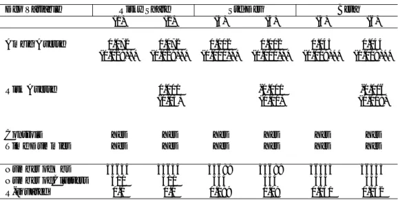
We further investigate the determinants of these di¤erences by focusing on those contracts which contain some risky assets. Results are presented in Table 8, which follows the same structure as Table 7. We …rst notice that results are larger in magnitude, as one would expect given that the variation in returns in a given month comes from risky contracts. As shown in columns (1)-(4), the positive impact of ambiguity aversion is driven by those contracts which contain risky assets. In these contracts, ambiguity averse investors experience about 0:035% higher returns per month (that is, about 0:51% per year). The e¤ect of risk aversion is negative and of similar magnitude.
As in Table 7, we then look at heterogeneous impacts with respect to Good Times. Estimates in column (6) show that ambiguity aversion leads to 0:2% higher returns in good times and to 0:13% lower returns in bad times. That is the case even when controlling for the riskiness of the contract.27
These results are perhaps surprising in light of the theoretical literature mentioned above on under diversi…cation, which would predict lower (risk-adjusted) returns. They are however consistent with the evidence we have presented earlier that ambiguity averse investors tend to choose riskier con-tracts, and in particular to hold portfolios with a higher beta. Overall, their returns are higher, but at the same time they are more sensitive to market trends.
6
Discussion
In this section, we wish to address two issues. First, whether our results may be biased by omitted behavioral characteristics. Second, whether our results can be considered representative of households’ …nancial behaviors in their broader portfolio.
6.1 Alternative behavioral traits
In principle, our previous estimates may be driven by factors correlated with ambiguity aversion and omitted from our regressions. This is of course a di¢ cult issue to resolve completely without experimental data. A …rst partial response is to notice that estimates do not seem sensitive to the inclusion or exclusion of various controls. This is what one would expect given that, as shown in Table 2, ambiguity aversion does not correlate much with standard demographic variables.
2 7
We only report the results in which we control for the standard deviation of the returns. Controlling for the risky share or for beta does not change our coe¢ cients of interest.
On the other hand, ambiguity preferences may be related to other be-havioral traits which we have not considered in our main analysis. First, ambiguity aversion may be related to sophistication: Halevy (2007) shows that probabilistically sophisticated subjects tend to be neutral towards am-biguity; Chew, Ratchford and Sagi (2013) show that only sophisticated sub-jects react to ambiguity as less sophisticated subsub-jects fail to perceive its mere presence. Second, ambiguity aversion may be related to (lack of) con-…dence. Heath and Tversky (1991) and Fox and Tversky (1995) show that ambiguity aversion may stem from the perceived lack of knowledge about the context. Third, in the spirit of Halevy (2008), ambiguity may be related to present biased preferences (see Cohen, Tallon and Vergnaud (2011) for an empirical investigation).
In order to dig further in this direction, we build some measures of so-phistication, con…dence, and time preference based on our survey questions. As for sophistication, we exploit a question in which we asked to compute compound interests. Assuming that one invested 1000 euros at a rate of 2% per year, subjects were asked how much money would be available after one year and after …ve years. The variable Compute Interest is a dummy equal to 1 if the respondent answered correctly (see Appendix 8.1 for details).
As for con…dence, we have asked a series of 10 true/false questions in-cluding whether holding shares gives the right to a …xed revenue; whether the value of the CAC40 Index has increased during 2009; whether the UK is part of the Euro area (the complete list and the exact formulation is reported in Appendix 8.1). Then, we have asked respondents how many questions they thought they answered correctly. Our measure of con…dence is based on the di¤erence between the subjective estimate and the actual number of correct answers. We construct the dummy Con…dence which is equal to one if the subject displays a level of con…dence above the median in the sample (that is equal to zero).
Finally, we capture present biased preferences by asking subjects to choose (hypothetically) between smaller gains today vs. larger gains in one month, and then between the same gains in 12 vs. 13 months. The variable Hyperbolic is a dummy equal to 1 if the subject prefers smaller gains today but higher gains when both alternatives are delayed.
While investigating the e¤ects of all these traits on portfolio choices re-mains beyond the scope of the present analysis, we here address the more limited issue of whether our coe¢ cients of interest are a¤ected by the inclu-sion of these extra variables. Results appear in Table 9, in which we re-run the main regressions of Section 5 adding the additional behavioral traits as controls. In column 1, the dependent variable captures the propensity to hold a risky contract (as in Table 3, column 3). In column 2, we look at the fraction of wealth invested in risky assets conditional on risk taking (as in Table 3, column 6); in column 3, we consider the change in risk exposure over time (as in Table 5, column 1); in column 4, we look at the direction
of rebalancing (as in Table 6, column 3). Finally, as in Tables 7 and 8, we consider monthly returns both overall (column 5) and conditional on risk taking (column 6).
The additional behavioral traits seem to explain little of the observed portfolio choices, and results are basically unchanged relative to the baseline speci…cations in Section 5.28 The e¤ects of ambiguity aversion are robust to the inclusion of our measures of sophistication, con…dence, and time prefer-ences.
6.2 Representativeness
As stressed, our results are based on the behavior observed within the com-pany and, as in most studies employing administrative data, we lack a full picture of households’portfolio or even more generally of their exposure to risk in other dimensions. One may then question whether what we observe within the company should be considered representative of households’be-haviors in their overall portfolios.
As a step towards answering this question, we exploit the information collected in our survey on households’…nancial assets and total wealth. We can estimate the fraction of wealth that the household has invested in the company, and check whether the e¤ects of ambiguity and risk preferences are di¤erent for those who have invested a lot vs. little of their wealth. If our estimates were driven by those with low investment in the company, our previous results may not be considered as very representative.29
In our survey, respondents were asked to report the value of their total wealth within a range. In order to de…ne the fraction of wealth invested, we need to build a point estimate. We consider the midpoint in each interval, except for the highest interval (where clients report wealth of 1 million euros or above) where we consider the minimum of the interval.30 In a similar way, we construct point estimates for the value of …nancial assets. We then compare these …gures to the value of the contracts held in the company as of August 2010 (around the time when the survey was conducted). According to these estimates, the median client holds 37% of his …nancial assets and 6% of his total wealth in the company. For each client, we then de…ne the dummy Low Invest as being equal to one if the value of his contracts is lower than 6% of his total wealth.31 In particular, we are interested in exploring
2 8
Similar results obtain by including the additional behavioral traits one by one.
2 9
Alternatively, one may invoke a form narrow framing whereby each asset (here, an assurance vie contract) is treated by households in isolation from the rest of their portfolio. For evidence of narrow framing, see e.g. Kahneman and Lovallo (1993), Barberis, Huang and Thaler (2006) and Choi, Laibson and Madrian (2009).
3 0
We have also considered the minimum or the maximum in the interval and the fol-lowing results are not a¤ected.
3 1
Similar results would obtain by constructing the dummy based on the value of the contracts relative to the client’s …nancial assets as well as by using the value of contracts
the interaction between Low Invest and ambiguity preferences.
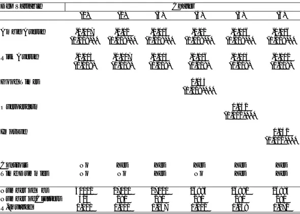
Results are reported in Table 10. The coe¢ cient on Ambig Averse de-scribes the e¤ect of ambiguity aversion on those clients who have a large fraction of their wealth invested in the company. The coe¢ cient on Low In-vest*Ambig describes the di¤erential impact of ambiguity aversion on those with a small fraction of wealth invested in the company. Similarly, for the coe¢ cients on Risk Averse.
As in Table 9, the dependent variables relate to the main results of the previous analysis. That is, we keep the same speci…cations as in Section 5 and investigate the e¤ects on the propensity to hold a risky contract (column 1), the fraction of wealth invested in risky assets (column 2), the change in risk exposure over time (column 3), the direction of rebalancing (column 4) and the monthly returns both overall (column 5) and conditional on risk taking (column 6).
In column 1, we observe that ambiguity averse clients with a large frac-tion of wealth invested are less likely to hold risky contracts while the op-posite is true for those with low wealth invested. However, as in the main analysis (Table 3, column 3), estimates are not statistically di¤erent from zero.
In columns (2)-(6), we see that our main results hold in the subsample of investors with a large fraction of wealth in the company, and that the e¤ects of ambiguity aversion are not signi…cantly di¤erent for those with a low fraction invested. Moreover, in magnitude, the estimated e¤ects on those with large investments are slightly bigger than the estimates obtained on the entire sample.
Overall, the e¤ects of ambiguity aversion do not seem to vary substan-tially depending on the fraction of wealth invested in the company. If any-thing, results are sometimes stronger on clients with large investments, for which arguably the observed portfolio is more representative of the overall portfolio. This suggests that the behaviors we observe within the company are (broadly) consistent with the behaviors of the households in their global portfolio.
7
Conclusion
We have explored the empirical relation between ambiguity aversion, risk aversion and portfolio choices. For this purpose, we have exploited an origi-nal data set in which administrative panel data obtained from a large French company are matched with survey data on preferences over ambiguity and risk. We have investigated in particular how these preferences a¤ect house-holds’ choices in terms of risk exposure, portfolio rebalancing as well as
the performance of their assets. We have shown that, conditional on par-ticipation, ambiguity averse individuals tend to choose riskier contracts. Moreover, they are more likely to rebalance their portfolio in a contrarian direction relative to the market. Accordingly, their exposure to risk is more stable over time. Finally, we have shown that ambiguity averse individuals experience higher market returns in good times and lower returns in bad times. The e¤ects of risk aversion are often very di¤erent both in sign and in magnitude.
As detailed above, some of these results lend support to existing theories of ambiguity aversion and portfolio choices. Other results, like increased risk taking and volatility of returns, are at …rst sight puzzling and we hope they can motivate further investigations. Both from a theoretical viewpoint, so as to better uncover the underlying mechanisms, and from an empirical view-point, so as to test their validity in other settings. This is only a …rst step towards an understanding of the empirical content of ambiguity preferences and of their relation with risk preferences. In our view, more research along these lines is clearly desirable.
References
Ahn, D., Choi, S., Gale, D. and Kariv, S. (2007), ‘Estimating ambiguity aversion in a portfolio choice experiment’.
Alvarez, F., Guiso, L. and Lippi, F. (2012), ‘Durable consumption and asset management with transaction and observation costs’, American Eco-nomic Review 102(5), 2272–2300.
Arrondel, L., Borgy, V. and Savignac, F. (2012), ‘L’épargnant au bord de la crise’, Revue d’économie …nancière 108(4), 69–90.
Barberis, N., Huang, M. and Thaler, R. H. (2006), ‘Individual preferences, monetary gambles, and stock market participation: A case for narrow framing’, American Economic Review 96(4), 1069–1090.
Barseghyan, L., Molinari, F., O’Donoghue, T. and Teitelbaum, J. C. (2013), ‘The nature of risk preferences: Evidence from insurance choices’, American Economic Review 103(6), 2499–2529.
Barseghyan, L., Molinari, F. and Teitelbaum, J. C. (2014), ‘Inference under stability of risk preferences’.
Barsky, R. B., Juster, F. T., Kimball, M. S. and Shapiro, M. D. (1997), ‘Preference parameters and behavioral heterogeneity: An experimental approach in the health and retirement study’, Quarterly Journal of Economics 112(2), 537–579.
Bauer, R. and Smeets, P. (2014), ‘Social identi…cation and investment deci-sions’.
Bossaerts, P., Ghirardato, P., Guarnaschelli, S. and Zame, W. R. (2010), ‘Ambiguity in asset markets: Theory and experiment’, Review of Fi-nancial Studies 23(4), 1325–1359.
Boyle, P., Garlappi, L., Uppal, R. and Wang, T. (2012), ‘Keynes meets markowitz: The trade-o¤ between familiarity and diversi…cation’, Man-agement Science 58(2), 253–272.
Butler, J. V., Guiso, L. and Jappelli, T. (2012), ‘The role of intuition and reasoning in driving aversion to risk and ambiguity’, Theory and Deci-sion - forthcoming .
Caballero, R. J. and Krishnamurthy, A. (2008), ‘Collective risk management in a ‡ight to quality episode’, Journal of Finance 63(5), 2195–2230. Caballero, R. J. and Simsek, A. (2013), ‘Fire sales in a model of complexity’,
Journal of Finance 68(6), 2549–2587.
Calvet, L. E., Campbell, J. Y. and Sodini, P. (2007), ‘Down or out: Assessing the welfare costs of household investment mistakes’, Journal of Political Economy 115(5), 707–747.
Calvet, L. E., Campbell, J. Y. and Sodini, P. (2009), ‘Fight or ‡ight? portfo-lio rebalancing by individual investors’, Quarterly Journal of Economics 124(1), 301–348.
Campbell, J. Y. (2006), ‘Household …nance’, Journal of Finance 61(4), 1553–1604.
Campbell, J. Y., Jackson, H. E., Madrian, B. C. and Tufano, P. (2011), ‘Consumer …nancial protection’, Journal of Economic Perspectives 25(1), 91–114.
Campbell, J. Y. and Viceira, L. M. (2002), Strategic asset allocation: port-folio choice for long-term investors, Oxford University Press.
Chew, S. H., Ratchford, M. and Sagi, J. S. (2013), ‘You need to recognize ambiguity to avoid it’.
Choi, J. J., Laibson, D. and Madrian, B. C. (2009), ‘Mental accounting in portfolio choice: Evidence from a ‡ypaper e¤ect’, American Economic Review 99(5), 2085–95.
Cohen, A. and Einav, L. (2007), ‘Estimating risk preferences from deductible choice’, American Economic Review 97(3), 745–788.
Cohen, M., Tallon, J.-M. and Vergnaud, J.-C. (2011), ‘An experimental investigation of imprecision attitude and its relation with risk attitude and impatience’, Theory and Decision 71(1), 81–109.
Collard, F., Mukerji, S., Sheppard, K. and Tallon, J.-M. (2012), ‘Ambiguity and the historical equity premium’.
Condie, S. (2008), ‘Living with ambiguity: prices and survival when in-vestors have heterogeneous preferences for ambiguity’, Economic The-ory 36(1), 81–108.
Condie, S. and Ganguli, J. V. (2012), ‘The pricing e¤ects of ambiguous private information’.
Dimmock, S. G., Kouwenberg, R., Mitchell, O. S. and Peijnenburg, K. (2013), ‘Ambiguity aversion and household portfolio choice: Empiri-cal evidence’.
Dimmock, S. G., Kouwenberg, R. and Wakker, P. P. (2013), ‘Ambiguity attitudes in a large representative sample’.
Dorn, D. and Huberman, G. (2005), ‘Talk and action: What individual investors say and what they do’, Review of Finance 9(4), 437–481. Dow, J. and Werlang, S. R. (1992), ‘Uncertainty aversion, risk aversion, and
the optimal choice of portfolio’, Econometrica 60(1), 197–204.
Epstein, L. G. and Ji, S. (2013), ‘Ambiguous volatility and asset pricing in continuous time’, Review of Financial Studies 26(7), 1740–1786. Epstein, L. G. and Schneider, M. (2010), ‘Ambiguity and asset markets’,
Annual Review of Financial Economics 2(1), 315–346.
Etner, J., Jeleva, M. and Tallon, J.-M. (2012), ‘Decision theory under am-biguity’, Journal of Economic Surveys 26(2), 234–270.
Fox, C. R. and Tversky, A. (1995), ‘Ambiguity aversion and comparative ignorance’, Quarterly Journal of Economics 110(3), 585–603.
Gajdos, T., Hayashi, T., Tallon, J.-M. and Vergnaud, J.-C. (2008), ‘At-titude toward imprecise information’, Journal of Economic Theory 140(1), 27–65.
Ganguli, J., Condie, S. and Illeditsch, P. K. (2012), ‘Information inertia’. Garlappi, L., Uppal, R. and Wang, T. (2007), ‘Portfolio selection with
pa-rameter and model uncertainty: A multi-prior approach’, Review of Financial Studies 20(1), 41–81.
Gollier, C. (2011), ‘Portfolio choices and asset prices: The comparative sta-tics of ambiguity aversion’, Review of Economic Studies 78(4), 1329– 1344.
Guerdijkova, A. and Sciubba, E. (2012), ‘Survival with ambiguity’.
Guidolin, M. and Rinaldi, F. (2013), ‘Ambiguity in asset pricing and portfo-lio choice: a review of the literature’, Theory and Decision 74(2), 183– 217.
Guiso, L., Sapienza, P. and Zingales, L. (2013), ‘Time varying risk aversion’. Guiso, L. and Sodini, P. (2012), ‘Household …nance: An emerging …eld’. Halevy, Y. (2007), ‘Ellsberg revisited: An experimental study’,
Economet-rica 75(2), 503–536.
Halevy, Y. (2008), ‘Strotz meets allais: Diminishing impatience and the certainty e¤ect’, American Economic Review 98(3), 1145–62.
Heath, C. and Tversky, A. (1991), ‘Preference and belief: Ambiguity and competence in choice under uncertainty’, Journal of Risk and Uncer-tainty 4(1), 5–28.
Ho¤mann, A. O., Post, T. and Pennings, J. M. (2013), ‘Individual investor perceptions and behavior during the …nancial crisis’, Journal of Banking & Finance 37(1), 60–74.
Hurd, M., Van Rooij, M. and Winter, J. (2011), ‘Stock market expectations of dutch households’, Journal of Applied Econometrics 26(3), 416–436. Illeditsch, P. K. (2011), ‘Ambiguous information, portfolio inertia, and
ex-cess volatility’, Journal of Finance 66(6), 2213–2247.
Ju, N. and Miao, J. (2012), ‘Ambiguity, learning, and asset returns’, Econo-metrica 80(2), 559–591.
Kahneman, D. and Lovallo, D. (1993), ‘Timid choices and bold forecasts: A cognitive perspective on risk taking’, Management science 39(1), 17–31. Klibano¤, P., Marinacci, M. and Mukerji, S. (2005), ‘A smooth model of
decision making under ambiguity’, Econometrica 73(6), 1849–1892. Knight, F. H. (1921), ‘Risk, uncertainty and pro…t’, New York: Hart,
Scha¤ ner and Marx .
Lin, Q. and Riedel, F. (2014), ‘Optimal consumption and portfolio choice with ambiguity’, Institute of Mathematical Economics Working Paper No 497 .