European integration, FDI and the geography of French trade

HAL Id: halshs-00586834

https://halshs.archives-ouvertes.fr/halshs-00586834

Preprint submitted on 18 Apr 2011

HAL is a multi-disciplinary open access

archive for the deposit and dissemination of sci-entific research documents, whether they are pub-lished or not. The documents may come from teaching and research institutions in France or abroad, or from public or private research centers.

L’archive ouverte pluridisciplinaire HAL, est destinée au dépôt et à la diffusion de documents scientifiques de niveau recherche, publiés ou non, émanant des établissements d’enseignement et de recherche français ou étrangers, des laboratoires publics ou privés.

European integration, FDI and the geography of French

trade

Miren Lafourcade, Elisenda Paluzie

To cite this version:

Miren Lafourcade, Elisenda Paluzie. European integration, FDI and the geography of French trade. 2008. �halshs-00586834�

WORKING PAPER N° 2008 - 13

European integration, FDI and the geography of French trade

Miren Lafourcade

Elisenda Paluzie

JEL Codes: F15, F23, R12, R58

Keywords: trade, gravity, border regions, European

integration, foreign direct investment

PARIS

-

LABORATOIRE D’ECONOMIE APPLIQUÉE - INRA

48,BD JOURDAN –E.N.S.–75014PARIS TÉL. :33(0)143136300 – FAX :33(0)143136310

European Integration, FDI and the Geography of French Trade

Miren Lafourcade

_{Elisenda Paluzie}

March 27, 2008

Abstract

This paper uses an augmented gravity model to investigate whether the 1978-2000 process of European integration has changed the geography of trade within France, with a particular focus on the trends experienced by border regions. We support the conclusion that, once controlled for bilateral distance, origin- and destination-specific characteristics, French border regions trade on average 72% more with nearby countries than predicted by the gravity norm. They perform even better (114%) if they have good cross-border transport connections to the neighboring country. However, this outperformance eroded drastically for the French border regions located at the pe-riphery of Europe throughout integration. We show that this trend is partly due to a decreasing propensity of foreign affiliates to trade with their home country. This trade reorientation is less pronounced for the Belgian-Luxembourgian and German firms located in the regions which have better access to the EU core.

JEL classification: F15, F23, R12, R58.

Keywords: Trade, Gravity, Border regions, European Integration, Foreign Direct Investment.

∗_{This paper has been prepared as part of a PREDIT research contract (Grant No:04-MT-5036). We would like to}

thank the French Ministry of Transport, specially Alain Sauvant and Micheline Travet, for providing us with French trade data in return for financial contractual obligations and strict confidentiality. We also acknowledge the French Government Agency For International Investment (and more particularly David Cousquer and Clotilde Lainard) and Thierry Mayer for their kind help in gathering data. We are indebted to Anthony Briant, Melika Ben Salem, Pierre-Philippe Combes, Joan Costa, Laurent Gobillon, Giordano Mion, Jordi Pons, Muriel Roger, Egle Tafenau and Daniel Tirado for insightful suggestions. Conference participants in Glasgow (February 2005), Cagliari (May 2005), Kiel (June 2005), Barcelona (July 2005) and Amsterdam (August 2005) provided us with fruitful comments. Financial supports from the CEPR Research Network on The Economic Geography of Europe: Measurement, Testing and Policy Simulations, funded by the European Commission under the Research Training Network Programme (Contract No: HPRN-CT-2000-00069), from the Spanish Ministry of Science and Technology (Project SEC2002-03212), the Spanish Ministry of Education (Project SEJ2005-03196/ECON) and the Catalan Government (2005SGR-00460) are also gratefully acknowledged.

†_{Corresponding author. University of Valenciennes and Paris School of Economics (PSE). PSE, 48 Bd. Jourdan,}

75014 Paris, France. lafourcade@pse.ens.fr. http://www.enpc.fr/ceras/lafourcade/.

1

Introduction

The recent wave of European eastward enlargement came along with an increasing fear of outsourcing to the new entrants. This makes prominent the question of how European integration is likely to affect the geography of economic activities. As the empirical evidence focused overwhelmingly on the post-integration re-allocation effects between old and new member countries, this paper aims to extend the assessment to the context of regions within countries. A particular focus is put on whether the border regions located at the interface of integrating countries expanded or suffered consequently to their shift from a peripheral position within France to a central location within the common market. Our approach is also innovative in that it considers foreign direct investment and cross-border transport infrastructure as possible channels conveying regional trade differentials. Economic integration, by improving market accessibility and alleviating impediments to both trade and multinational activity, induces multinational firms to invest in the new regional bloc. Since foreign affiliates are more likely to locate according to “market potentials”, as recently emphasized by Head and Mayer (2004), the border regions located at the core of rich Europe might benefit from the over-representation of outside firms and, if FDI and trade are complementary activities, from trade expansion. As for policy prospects, the question of whether border regions exhibit specific attractiveness for economic activities is of eminent significance in the context of the adoption by the European Commission of multiple entrepreneurship, trade and transport cross-border programmes under the new cohesion policy 2007-2013. To facilitate cross-border cooperation, the EU has indeed recently created a new legal entity, the European Group-ing for Territorial Cooperation (EGTC) enablGroup-ing to group the authorities of various member states, without the need of prior international agreements.

The issue of whether economic integration might favor or hamper border regions is controversial. From a theoretical point of view, the New Economic Geography (henceforth NEG) has sought to extend the usual 2-country (or 2-region) setting to frameworks in which both inter- and intra-national inequalities are assessed. In a model with a foreign country and a home country, each composed of two equidistant domestic regions (the core and the periphery), Krugman and Livas (1996) show that trade liberalization between countries favors the regional dispersion of increasing return to scale activities between the core and the periphery of each country. Hence, the peripheral region could reap from the magnification of urban congestion within the core. However this result is not robust: when the dispersion force materializes into immobile workers, instead of urban congestion, catastrophic agglomeration may occur, as shown by Monfort and Nicolini (2000) and Paluzie (2001). In a slightly modified setting, in which one of the two domestic regions is farther away from the foreign market than the other, Crozet and Koenig (2004) show that trade liberalization drives domestic firms to the region

closer to the border, unless competition pressure from the foreign market is too fierce. As opening up to trade with a foreign economy increases exports (foreign demand) and imports (foreign supply), the impact of trade liberalization is the result of two counteracting forces: increased market access (favorable to export production) and increased import competition (negative for domestic producers that compete with foreign supply).

Nonetheless, the core-periphery models of the Krugman’s type are not only known for the extreme result that trade costs reduction would yield catastrophic agglomeration, but also for their analytical intractability. Hence, recent studies have tried both to attenuate centripetal forces and to provide analytical solutions to the models. For instance, Br¨ulhart et al. (2004) build a 3-region setting in which the manufacturing sector uses mobile human capital as the fixed cost and immobile workers as the variable cost of production. They find that, for most parameter configurations, trade liberalization favors the concentration of human capital in the border region. However, this mechanism is not deterministic: A sufficiently strong pre-liberalization concentration of economic activity in the interior region can make this concentration globally stable, and predicts even more agglomeration in this region. Behrens et al. (in press) develop a 2-country 4-region model in which low inter-country trade costs is shown to promote regional dispersion when inter-regional trade costs are high enough. Behrens et al. (2006) use the same model to investigate the role of “gate” regions, through which goods are shipped to the international market. If one country is endowed with such a region, the latter benefits from agglomeration when the country is well integrated whereas, in the other case, it is the landlocked region. Therefore, theory has not reached a consensus on whether or not border regions might benefit from integration processes. Hence, empirical analysis is even more crucial to identify the main mechanisms at work.

The main empirical approach consists in testing the NEG predictions of backward (demand) linkage effects:1 the better a region’s access to large markets, the higher its factor prices, output, or a mix of the two. Therefore, regional wage gradients, which were initially decreasing monotonously from center to periphery, might possibly reverse consequently to changes in trade regimes and market potentials. As for output variables, adjustments are driven by the number of firms, and regions with good access to foreign markets end up with a higher share of activities. Regarding North-America, Hanson (1996a, 1996b, 1997, 2001) are among the pioneer empirical studies assessing whether the NAFTA process entailed changes in wages or employment within participating countries. While they provide strong evidence of jobs relocation by the two sides of the U.S.-Mexico border following NAFTA, they do not yet support unequivocally the wage gradients reversal prediction. EU prospects concern

mostly the recent eastward enlargement and the fear that, as the borders of CEE countries become internal to the EU, economic activities could shift towards Eastern border locations, eventually at the expense of Western border regions. For instance, Br¨ulhart and Koenig (2006) compare the wage gradients of five accession countries (Czech Republic, Hungary, Poland, Slovenia and Slovakia) to those of incumbent EU countries, for the period 1996-2000. They find that concentration in the capital regions is significantly stronger in the former and that nominal wages are higher in the border regions of incumbent EU countries. Hence, they conjecture that market forces would likely favor Eastern border regions. Based on simulated changes in the market accessibility of EU27 regions, Niebuhr (2005) also supports the conjecture that border regions could experience above-average integration benefits due to their favorable access to foreign markets. A noticeable exception to the eastward focus is the recent work by Overman and Winters (2003, 2005), who examine whether the UK’s accession to the EEC in 1973 impacted the location of domestic manufacturing activities within the UK. Accession is shown to have a mitigated effect: even though manufacturing activities might have relocated south-eastwards, several industries also retreated north-westwards, because of increased import competition. Therefore, the empirical estimation of backward linkages, both in the factor price version (wages) and quantity version (employment or production) indicates that regions bordering the largest and richest markets do seem to benefit from economic integration with them. By contrast, the results for regions bordering poorer markets are more mixed. Some of them, like the South of the US, experience positive effects while for others, particularly in Eastern Europe, the impact might be negative.

Our empirical approach is different in that first, we focus on the western part of Europe and secondly, we concentrate on trade rather than on wage and employment issues. Post-integration changes in trade performances that would depend on where regions are located within countries have been rarely investigated. Two noticeable exceptions have to be mentioned. First, Coughlin and Wall (2003) distill the trade impact of NAFTA on the US states. Their conclusion is that, following NAFTA, 28 (36, respectively) U.S. states experienced a rise of more than 10% in their exports towards Mexico (Canada, respectively), while 8 (4, respectively) were negatively affected. However, the core-periphery nature of winners and losers is not assessed. In contrast, Egger and Pfaffermayr (2002) analyze the trade impact of the 1960-1998 process of EU integration, with a special focus on trade within and between the core and periphery countries. They find out that, while both core-periphery and intra-periphery countries benefited more from EU integration than intra-core countries, this positive effect reduced throughout the enlargement. The southern enlargement even turned to exert a negative effect on the intra-core volume of trade.

In line with Egger and Pfaffermayr (2002), we assess the trade differentials sparked by European integration, but we focus on the case of French regions. We develop an augmented gravity model in

which European integration is materialized through the reduction of FDI barriers. We then quantify the trade performance of border regions as their deviation from the value of trade predicted by this gravity norm. We find evidence that, everything else equal, French border regions trade on average 72% more with nearby countries than predicted by the norm, and even more (114%) if they have good cross-border transport connections. However, the process of European integration has coincided with a large decrease in this trade overperformance over the period 1978-2000. This trend was driven by the drastic fall in the deviations experienced by the most peripheral French border regions within the EU. Neither the Single European Act nor the completion of the Single Market were sufficient to counterbalance the decline. We find that these trade differentials can partly be attributed to FDI regional patterns, and more precisely to a decreasing scope for trading with the home country. However, this trend is less pronounced for the Belgian-Luxembourgian and German firms located at the vicinity of the EU core.

The remainder of the paper proceeds as follows. Section 2 provides some stylized evidence on the suitability of the gravity framework for the study of the interplay between trade performances and FDI. Section 3 describes the augmented gravity model, as well as the data and methodological issues. Section 4 provides two sets of results for France. The first set relates to the 1978-2000 long-span evolution of trade differentials between border and interior regions, whereas the second set analyzes more specifically the role of inward FDI in the period 1993-2000. Section 5 concludes.

2

Trade and FDI patterns of French regions: Stylized evidence

A detailed assessment on whether integration is likely to affect the internal geography of trade requires a thorough theoretical and econometric analysis, that we will seek to provide in subsequent sections. However, if border regions experience specific trends arising from the counteracting forces described in the Introduction, we should be able to pick up them with the naked eye. Section 2 therefore provides a set of stylized facts on the trade and FDI patterns of French regions.

2.1 Trade specialization patterns by country

To illustrate that proximity is a clear catalyst for trade, a brief look at the relative trade performances of regions inside France is instructive.2 _{So as to assess the relative specialization of regions across}

partner countries, we compute the following trade index. Let J denote the trade partner country of 2_{As we seek for trade differentials depending on whether regions border a country or not, we examine only the six}

EU countries neighboring France: Belgium, Luxembourg, Germany, United-Kingdom, Spain and Italy. Due to data constraints, we treat Belgium and Luxembourg as a single partner country for French regions. Appendix A presents the data sources.

region i. We define s_iJ = F_iJ/P_i∈IF_iJ as the share of region i in the country I’s trade with country J, and xi = P KFiK/ P i∈I P

KFiK as its share in the country I’s international trade. The simplest

way to measure how much the trade of region i is oriented towards the partner country J, and to compare this trade intensity across countries, is to compute the following Balassa Trade Specialization Index:

T SIiJ = s_xiJ

i × 100. (1)

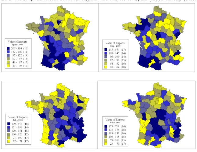
Values above 100 mean that region i trades relatively more with country J than would be predicted by its share in international trade. Figures 1 and 2 exhibit the patterns obtained in 2000.

Figure 1: Trade specialization of French regions with respect to: Spain (top) and Italy (bottom)

Source: Authors’ computations based on data from the SITRAM database (French Ministry of Transport). See Appendix A for further details.

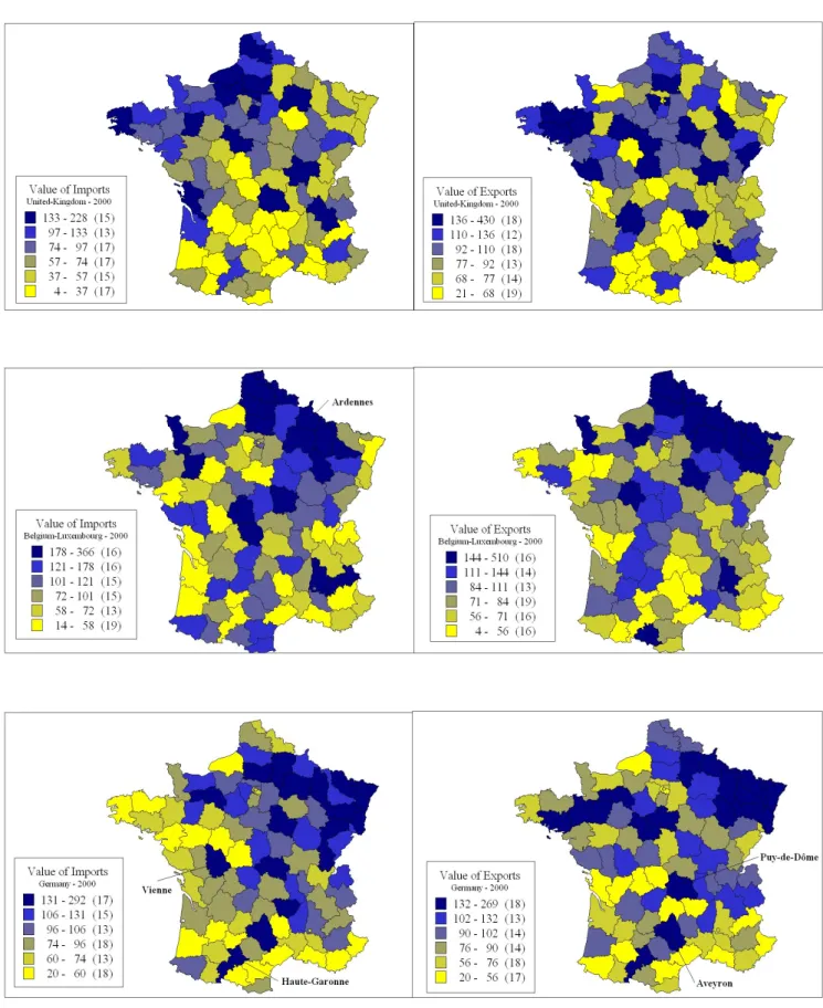
The gravity pattern of trade is striking: regardless of the direction of trade, border regions always outperform “vis-`a-vis” the countries with which they share a frontier. This pattern is especially clear at the French borders with Belgium-Luxembourg and Germany. For instance, with a TSI of respectively 280 for exports and 355 for imports, the French NUTS3 “Ardennes”, which borders Belgium, is almost four times more export-oriented towards this country than with the rest of the world.

Hence, proximity gives the agents located on both sides of the same frontier clear incentives to trade. Sometimes however, specific border regions have a surprisingly low TSI. For instance, in the NUTS3 region of “Haute-Garonne”, which hosts Toulouse and has a border with Spain, mountains in the central part of the Pyrenees represent a major geographic obstacle and make cross-border transport particularly difficult. Therefore, a strict contiguity criterion is not always sufficient to embody the real border nature of regions, as the geography of frontiers may also deeply affect trade specializations.

Furthermore, interior regions sometimes present surprisingly high levels of specialization with regard to a partner country, in spite of being located very far away. One first plausible explanation is that cross-border input-output linkages might generate specific patterns which are not necessarily of the gravity type. For instance, the French central regions of “Puy de Dˆome” and “Vienne” exhibit a strong specialization of exports oriented towards Germany, probably due to the presence of the French firm Michelin, which produces equipment goods for German firms such as BMW, Daimler-Chrysler and Volkswagen A.G. A second explanation is that vertical outsourcing, which enables foreign investors to benefit from advantages other than reduced transport costs (such as low taxes, rents or wages) might also cause extreme specialization patterns. Foreign inward direct investment from neighboring countries is likely to boost trade due to input-output linkages between the foreign parent firm in the home country and its affiliates in the host region. For instance, the south region of “Haute-Garonne” comes out as the most specialized regarding exports to Germany, although it is located on the opposite side of this country. The reason may be that it hosts the European Aeronautic Defence and Space (EADS) consortium, of which the German firm Daimler-Chrysler owns more than 30%. Therefore, to compare the trade performance and orientation of regions we have to bear in mind that FDI might expand the trade of interior as well as of border regions. Next section focuses more specifically on this issue.

2.2 FDI specialization patterns by country

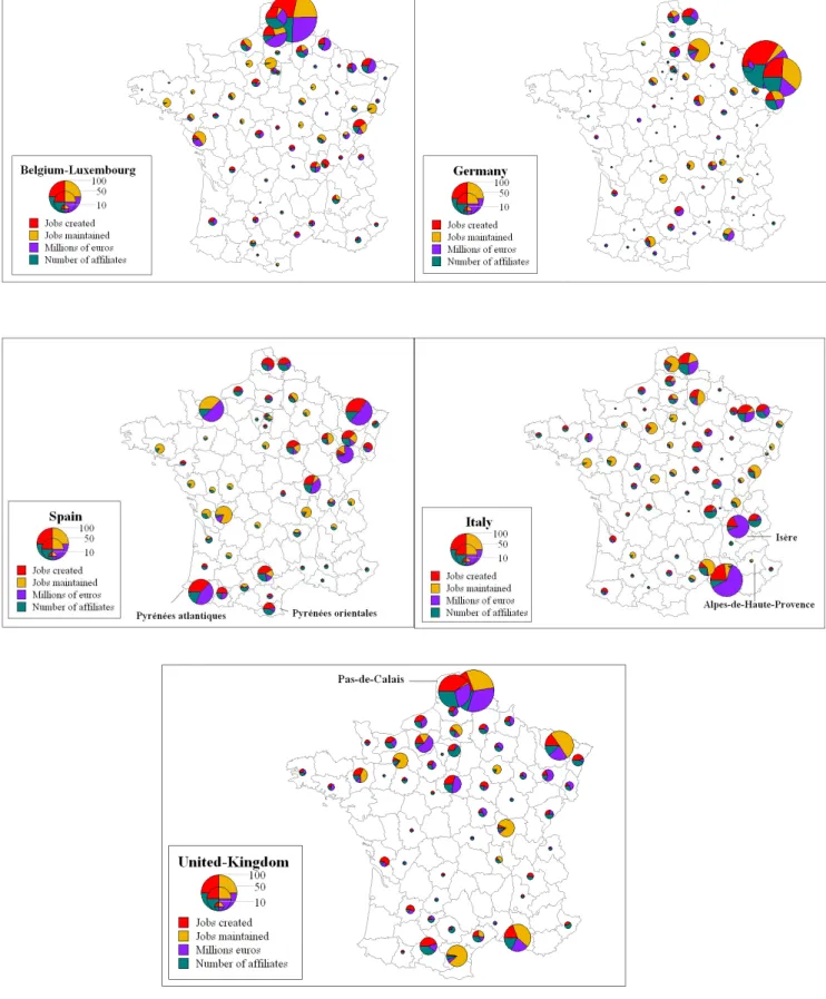
Figure 3 depicts the inward stocks of Foreign inward Direct Investment based on four different vari-ables: Number of foreign affiliates, created or saved related employment (hence, zero indicates green-field investment), and millions of euros invested.3

Figure 2: Trade specialization of French regions with respect to: United-Kingdom (top), Belgium-Luxembourg (middle) and Germany (bottom)

Figure 3: Regional stocks of FDI by country source in 2000 (in % of total FDI from the country)

Source: Authors’ computations based on data from the French Government Agency for International Investment (AFII). FDI flows (productive activities only) cumulated over 1993-2000. See Appendix A for further details.

Two striking features arise from this picture. First, regardless of their nationality, foreign firms have a clear preference for the regions located along the north-eastern frontier of France. These border regions present conducive conditions for investment as they benefit from good access to the richest internal French regions, due to the high density of highway infrastructures towards the French capital,4

and also to the core of Europe. As the propensity to invest increases with market potentials (Head and Mayer, 2004), the north-eastern French border represents a good trade-off between the desire to save on accessing French consumers and the costs of operating in rich European markets at the same time. Secondly, foreign firms also target the regions located at the other side of their home frontier, which may feed their trade expansion. As argued in Crozet et al. (2004), the similarity in cultures around the two sides of a same frontier is likely to distort FDI patterns at the benefit of the regions nearby home country. Gravity forces may even extend beyond such regions due to the spatial propagation of preferences. Other features such as natural geographic impediments may also increase the propensity of foreign firms to target some of the border regions at the expense of others, or to locate a bit further away from the border. Hence, Italian firms favor the “Is`ere” region at the expense of the mountainous “Alpes-de-Haute-Provence”, whereas Spanish firms clearly prefer to locate in “Pyr´en´ees atlantiques” and “Pyr´en´ees orientales”, where smoother relief allows for pass-roads. The same trend is very salient for British firms, who prefer to locate in “Pas-de-Calais” region, which benefits from the Euro-tunnel connection to the UK. These features stress the heterogeneity of border regions, and the need to qualify their border nature according to the geography of frontiers.

Finally, it is worth noting that exceptions to these two trends, which are found in some regions, confirm some of the conjectures given in section 2.1. For instance, despite its remoteness, the south-central region of “Aveyron”, whose exports are strongly oriented towards Germany, hosts a large share of the total German FDI.5

3

Trade specifications, data and econometric issues

Section 3 presents the theoretical mechanisms underpinning the interplay between economic integra-tion, multinational activity and trade (Section 3.1), and provides some clue on the data and estimation issues (Section 3.2).

4_{See Combes and Lafourcade (2005) for a more detailed picture of the relative transport accessibility of French regions.} 5_{As is well known, Bosch is one of the German affiliates located in this region.}

3.1 The augmented gravity model

The representative utility in region i depends on the consumption of the nJtvarieties produced in each

foreign partner country J, ciJt.6 Varieties are differentiated with a constant elasticity of substitution

(CES). Goods being heterogeneous across countries, we use the Armington’s (1969) assumption that consumers might prefer the varieties produced in some countries at the expense of others: parameter a_iJtcaptures the preference bias of consumers in region i with respect to the varieties produced in J. The utility function in region i is:

Uit = Ã X J X nJt (aiJtciJt) σ−1 σ ! σ σ−1 , (2)

where σ > 1 is the elasticity of substitution between the varieties produced abroad.

Let p_iJt denote the delivered price in region i of any variety produced in country J, τ_iJt, the ad valorem trade cost, and pJt the mill price in J. We have piJt= (1 + τiJt) pJt.

It is straightforward to obtain the following expression for imports originating from J:

ciJt = citPitσ−1nJtp1−σJt aσ−1iJt (1 + τiJt)1−σ, (3)

where cit =

P

J

P

hciJht is total demand in region i for varieties originating from all foreign sources,

and Pit, the price index in region i, Pit≡

¡P

Jaσ−1iJt nJtp1−σiJt

¢_1/(1−σ) .

We assume that trade costs are composed of two different elements: transport costs, TiJt, and

specific cross-border costs, BiJt:

(1 + τiJt)σ−1 = TiJtBiJt. (4)

Transport costs have the following symmetric structure: TiJt= TJit= (distiJ)δexp

¡

1 − β₁Tbord1iJ− β2Tbord2iJ

¢

, (5)

where bord1iJ and bord2iJ are contiguity dummies capturing the border nature of regions. bord1iJ = 1

indicates that the NUTS3 region i shares a frontier with country J (first-order contiguity criterion), while bord2iJ = 1 means that, absent strict contiguity, the NUTS3 region i belongs to a NUTS2

region that shares a frontier with country J (second-order contiguity criterion). Moreover, if, absent transport gateways, trade cannot transit through the border of region i to accede market J (due for 6_{In the rest of the paper, small letters will refer to regions and capital letters to countries. The subscript t indicates}

instance to mountains), the two previous dummies are set to 0, which means that region i is treated as interior and not border. Therefore, we capture the “real” border nature of regions by taking into account their endowments in cross-border infrastructures in addition to their location at the political frontier. As cross-border transport connections alleviate the cost of shipping goods through the border, parameters βT

1 and β2T are both expected to be positive. Finally, more standardly, transport costs

increase with the distance incurred to ship goods between region i and country J, distiJ.

Specific cross-border costs, B_iJt, include first tariffs t_IJt. The protection structure depends only on bilateral trade agreements signed by countries I and J, which are uniform across border and non-border regions. Advances in European integration are reflected in the progressive removal of tariffs, but also in the alleviation of informal barriers to trade, denoted ntbiJt, that might affect either border

or non-border regions differently. We assume:

B_iJt= (1 + t_IJt)(1 + ntb_iJt) = (1 + f di_iJt)−αB, (6) where f diiJt is a measure of the inward stock of bilateral foreign direct investment.7

The relationship between trade barriers and FDI is a rather disputed issue in theory (Neary, 2002; Faini, 2004). Consequently, there is no clear assertion on the question whether multinational activity and trade should be complements or substitutes.8 _{On one side, the reduction in trade barriers alleviates}

the costs for foreign firms of operating outside their home market, which should give multinationals more incentives to fragment production. If region i benefits from lower input costs relatively to other regions, it should be targeted for vertical outsourcing. If foreign affiliates trade back and forth with parent firms located in the home country, there should be a positive causation between FDI and both the imports and exports of the recipient region. Moreover, a number of recent models explain the propensity of more productive firms to self-select into multinational activity.9 _{This could generate an}

additional trade-expanding effect for the recipient regions. A huge body of empirical literature actually supports the evidence that multinational activity and trade would be complementary activities (Lipsey and Weiss, 1981, 1984; Pfaffermayr, 1996; Clausing, 2000; Head and Ries, 2001). However, on the other side, standard theory of multinational corporation predicts a proximity-concentration trade-off which leads firms to outsource production when trade barriers are large and scale economies at the plant level outpace scale economies at the industry level (Brainard, 1997). Therefore, horizontally-motivated 7_{The direction of FDI is therefore assumed to be the same as imports. A proper modeling of border barriers would}

require the addition of the outward stock, f diJit, which would entail more plausible asymmetric trade costs. However,

absent data, we have to restrict to inward FDI only.

8_{Forte (2004) provides an exhaustive survey of both the theoretical and empirical literatures on this question.} 9_{See among others Bernard et al. (2003), Melitz (2003), Helpman et al. (2004).}

overseas production could substitute for exports to the home country. In addition, if foreign affiliates deter the entry of local producers (for goods, as for production factors), multinational activities could also depress the domestic part of the region’s trade. Hence, we expect αB _{to be either positive}

or negative, depending on whether the complementarity-expanding effects offset the substitution-depressing influences.

Preferences integrate deterministic as well as stochastic elements: aσ−1_iJt = (1 + f diiJt)α

a

exp[β₁abord1iJ+ βa2bord2iJ+ εiJt], (7)

where εiJt is the random component. FDI affects these Armington preferences because it is more

likely to occur the more similar the home and the recipient markets are. In return, if the presence of multinationals is a conduit for both a better knowledge of foreign goods and a better adaptation of these goods to local tastes, parameter αa is expected to be positive. The border dummy bord1iJ

captures the existence of possibly close ties between consumers located on both sides of the same frontier. As the propagation of preferences might extend outside the frontier of strictly contiguous regions, especially if those are small areas, we also introduce bord2iJ. If consumers living in border

regions have a larger propensity to share the tastes of the nearby country than other regions, we expect parameters βa

1 and β2a to be both positive, though β2a should be of lower magnitude than β2a

due to the distance decay.

Taking logs and plugging back expressions (4), (5), (6) and (7) into equation (3), we obtain the following log-specification for imports:

ln ciJt = 1 + ln cit+ (σ − 1) ln Pit+ ln nJt+ (1 − σ) ln pJt

−δ ln distiJ + α ln (1 + f diiJt) + β1bord1iJ+ β2bord2iJ+ εiJt (8)

where α = αa_{+ α}B_{, β}

1 = β1T + β1a, β2 = β2T + β2a.

The bias in consumers’ preferences affects only the imports of varieties originating from nearby countries. Therefore, exports can be readily derived from the following restrictions: αa_{= β}a

1 = βa2 = 0.

3.2 Trade specifications and econometric issues

Equation (8) involves three groups of variables: Origin (J-specific), destination (i-specific) and “dyadic” (or bilateral iJ-specific). In order to tackle the problem that non-dyadic variables cit, Pit, nJt and pJt

destination-specific and origin-destination-specific variables by two groups of dummies.10 _{The import specification we estimate}

is the following:

ln ciJt = θ + fit+ fJt− δ ln distiJ+ α ln (1 + f diiJt) + β1bord1iJ+ β2bord2iJ+ ft+ εiJt, (9)

where ftis a year-dummy capturing the unobserved time-dependent factors affecting flows identically

across regions and countries, and where fit and fJt are respectively destination- and origin-specific

dummies interacted with the previous.

Independently of trade direction, the FDI explanatory variable is potentially endogenous in equa-tion (9), as the locaequa-tion choice of foreign firms is likely to depend on the trade activity itself. To overcome this simultaneity problem, we use the method of instrument variables and estimate the model by 2SLS. Hence, we have to find at least one variable that is partially correlated with FDI (but not with trade), once all the other right-hand-side exogenous variables of equation (9) have been net-ted out. Therefore, the IV candidate must be dyadic (i.e. iJ-specific), otherwise it would be strictly collinear with either the origin or the destination fixed-effects.11 We choose the following instrument:

M P_iJt1993 = X k∈I(6=i) emp_kJt gtc1993 ki , (10)

where emp_kJt is the total employment of all the J affiliates located in region k, and gtc_iJ is the generalized domestic transport cost incurred to ship manufacturing goods from region i to region k in 1993.12 _{Therefore, M P}1993

iJt is a French market potential variable capturing the propensity of foreign

firms to locate at the vicinity of the largest affiliates from the same home country, which proved to be highly correlated with FDI location in previous empirical studies (for instance Crozet et al., 2004). To avoid any additional bias arising from potentially endogenous transport infrastructures (since greater amounts of public funds might be devoted to the main FDI recipient regions), we compute market potentials based on the value of transport costs at the beginning of the sample period, i.e. 1993.

The first-stage regression consists here in estimating the following FDI specification:

ln (1 + f di_iJt) = ρ + f_it+ f_Jt− γ ln dist_iJ+ φln (1 + M P_iJt) + ϕ₁bord_1iJ+ ϕ₂bord_2iJ+ f_t+ ξ_iJt. (11) 10_{Empirically, including fixed-effects is actually the most widely accepted means of obtaining theory-consistent}

es-timates for gravity equations. See for instance Bergstrand (1985), Hummels (1999), or Anderson and van Wincoop (2003).

11_{In standard empirical analysis (discrete choice or gravity models), FDI specifications include a set of variables}

related to the recipient region (local taxes, wages, GDP, ...) and to the home country. We cannot use such variables as instruments here, because they are already captured by either fit or fJt.

The IV estimator for α derives from the following second-stage regression:

ln ciJt= θ + fit+ fJt− δ ln distiJ + α[ln (1 + f did iJt)] + β1bord1iJ+ β2bord2iJ+ ft+ ²iJt. (12)

The IV estimator is consistent under the hypothesis that the market potential and FDI variables are effectively partially correlated. Absent additional exclusion restrictions, the model is just identified and, therefore, condition φ 6= 0 must hold.

3.3 Definition of border regions

As noted in Section 2, caution is needed to define border regions properly. Several French border regions, although they share a frontier with a neighboring country, do not necessarily benefit from a direct access to this country, mostly because of physical geography (sea, mountains, ...). Therefore, we run two sets of regressions that build on two different definitions of border regions. Firstly, we adopt a large definition based on a simple contiguity bilateral criterion.13 _{We consider that all}

the regions sharing a frontier with at least one neighboring country, by land or by sea, are border regions.14 _{Secondly, we restrict the definition of border regions to the subset of contiguous regions}

which are effectively well connected to the nearby country, i.e. the regions hosting good cross-border transport infrastructures (major highways, tunnels or harbors).15 _{Using the two sets of estimates, we}

can compare the trade performances of both types of border regions and quantify the contribution of transport corridors to these performances, a prominent issue for policy-makers.

4

The trade performance of border and non-border regions

In this section, we present two sets of estimations. In the first set, presented in Section 4.1, we analyze the trade performance of border regions relatively to interior regions over the whole period 1978-2000. Although this approach neglects the causal relationship between multinational activity and trade, it makes possible to break down the sample into different sub-periods and to analyze the changes in trade performances occurring throughout the successive integration episodes. By way of contrast, Section 4.2 provides further estimates which are structurally-consistent. However, due to data constraint, the relationship between trade performances and FDI can only be investigated properly for the period 1993-2000.

13_{See Appendix B for detailed listing and mapping.}

14_{With respect to the UK, we consider all regions bordering the English Channel.}

15_{See Appendix B for detailed listing and mapping. To avoid any bias due to the possible simultaneity of trade and}

4.1 Baseline regressions: 1978-2000

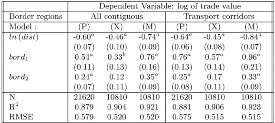
Table 1 reports the OLS estimates derived from estimating equation (9), absent FDI in the right-hand side explanatory variables. We consider the trade of French regions with the five neighboring countries of France. Hence, in our estimation, the trade partner country J can only be Belgium-Luxembourg, Germany, UK, Spain or Italy. Columns (P), (X) and (M) report the coefficients estimated over respectively pooled flows, exports and imports.

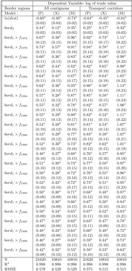
Table 1: The average trade outperformance of French border regions

Dependent Variable: log of trade value Border regions All contiguous Transport corridors Model : (P) (X) (M) (P) (X) (M) ln (dist) -0.60a _-0.46a _-0.74a _-0.64a _-0.45a _-0.84a (0.07) (0.10) (0.09) (0.06) (0.08) (0.07) bord1 0.54a 0.33b 0.76a 0.76a 0.57a 0.96a (0.11) (0.13) (0.16) (0.13) (0.14) (0.21) bord2 0.24a 0.12 0.35a 0.25a 0.17 0.33a (0.07) (0.11) (0.09) (0.08) (0.11) (0.09) N 21620 10810 10810 21620 10810 10810 R2 _{0.879 0.904 0.921 0.881 0.906 0.923} RMSE 0.579 0.520 0.520 0.575 0.515 0.515 Notes: (i) Specification estimated: ln (ciJt) = θ − δ ln (distiJ) + β1bord1iJ+ β2bord2iJ+ fit+ fJt+ ft+ εiJt. (ii) Heteroskedasticity-robust standard errors

in brackets, witha_,b_andc_{denoting significance at the 1%, 5% and 10% levels,}

respectively. Fixed-effects are not reported.

A first overall conclusion to be drawn from Table 1 is that, everything else equal, border regions trade substantially more with the country with whom they share a frontier than do interior regions. The magnitude of this trade outperformance is considerably larger for first-order than for second-order border regions (i.e. bord1 > bord2): the former trade on average 72% more ([exp(0.54) − 1] × 100)

than interior regions, whereas the trade deviation is 27% only ([exp(0.24) − 1] × 100) for the latter. As expected, border regions endowed with good cross-border transport connections outperform even better, with an average trade outperformance of 114% ([exp(0.76) − 1] × 100). Trade deviations with respect to the gravity norm are globally larger for imports than for exports, which means that βa

1 > 0 and β2a > 0 in equation (8). This is consistent with the model’s assumption that consumers’

preferences would be biased in favor of the differentiated goods imported from nearby countries or, in other words, that countries would actually export more to the regions located at the other side of their frontier than to other regions, due to “cultural” proximity.

Beyond simple average, one might wonder how relative trade performances have evolved over the last two decades of EU integration. A dynamic perspective is even more illuminating, given that NEG models mostly build on comparative statics and do not generally account for long-term evolutions.

The drawback of time-series analysis here is that different integration episodes might have affected French trade at the same time. Indeed, although EU reforms become effective at a formal date, their impact is actually largely anticipated, and changes are likely to occur even earlier than the time of implementation. Therefore, we cannot reasonably capture the changes induced by integration with a standard difference-in-difference approach. To overcome the issue of scheduling European integration, we choose to follow trade performances throughout the period 1978-2000 and to check whether significant changes occurred around the time of main formal reforms, that is around the Single European Act (1986), the Schengen Agreement (1990), the Maastricht (1992) treaty, and the successive EU enlargements to Greece (1981), Spain, Portugal (1986), Austria, Finland and Sweden (1996). More precisely, we adopt two different approaches. First, we keep on working with trade flows pooled over years. We thus interact border and time dummies so as to test for significant changes in the coefficients from year to year. Secondly, we undertake further estimations based on yearly trade sub-samples, in order to test whether the border regions located at the vicinity of the EU core exhibit specific trends in comparison with the border regions located at the periphery of western Europe.

Table 2 reports the results of the first set of estimations. Throughout the period 1978-2000, we observe a progressive fall in the trade outperformance of border regions. While the regions bordering a country used to trade around twice more with this country than their interior counterparts in 1978, they end with a lead of only 52.2% in 2000. The same declining trend is experienced by transport corridors, whose trade outperformances were cut up by nearly a half on the same period.

Hence, the benefits of acceding to new foreign markets would be offset by the loss induced by increasing import competition throughout the European process of integration. However, counter forces seem to have acted against the decline by the time of two main integration episodes, that is slightly before the Single European Act of 1986 and slightly after the Schengen Agreement of 1990.

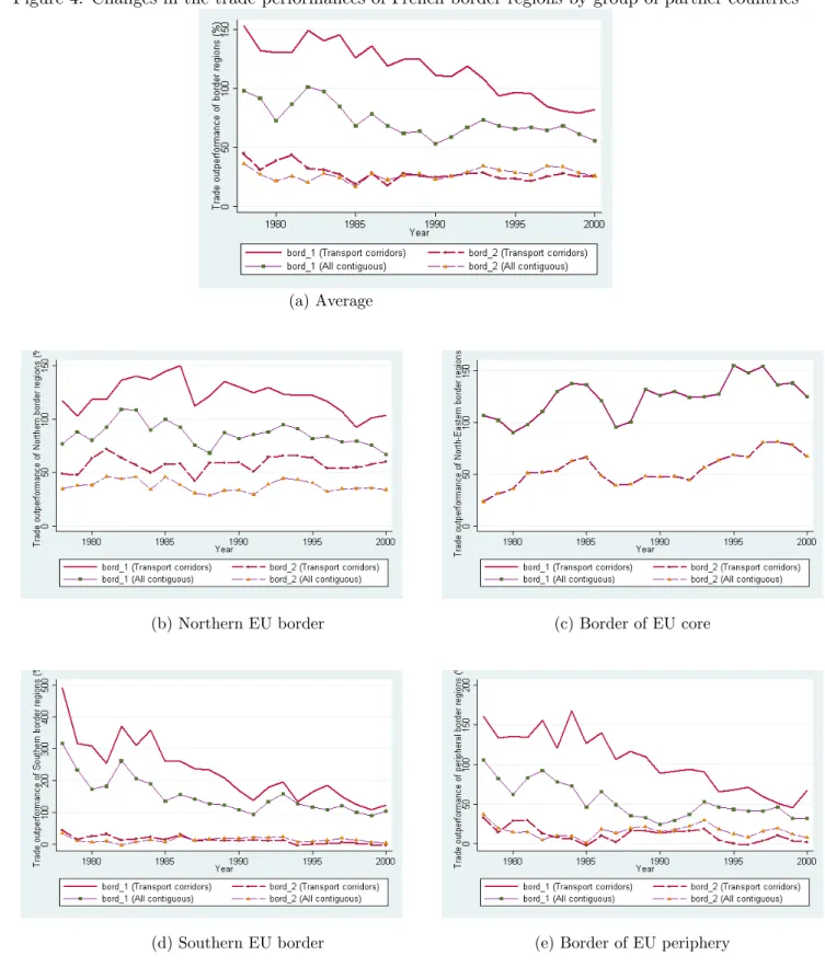
In the second set of estimations, we proceed with year-by-year regressions over pooled over imports and exports, for different sub-samples of partner countries. Figure 4-(a) reports the time changes in the average trade performances of border regions, computed as [exp(β) − 1] × 100, where β is the coefficient related to the year of estimation.16 The range of estimates is very similar to that obtained previously. In addition, we see that the gap between well and bad connected border regions narrows throughout the integration process (as reflected by converging thick and thin lines). The reason might be that “gateway” regions did not experience major infrastructure improvements during the period 1978-2000, while their counterparts did.17

Table 2: Time changes in the trade performance of French border regions

Dependent Variable: log of trade value Border regions All contiguous Transport corridors Model : (P) (X) (M) (P) (X) (M) ln(dist) -0.60a _-0.46a _-0.74a _-0.64a _-0.45a _-0.84a (0.02) (0.03) (0.02) (0.02) (0.02) (0.02) bord2 0.24a 0.12a 0.35a 0.25a 0.17a 0.33a (0.02) (0.03) (0.02) (0.02) (0.03) (0.02) bord1× f1978 0.67a 0.38b 0.96a 0.92a 0.73a 1.11a (0.12) (0.15) (0.16) (0.15) (0.17) (0.22) bord1× f1979 0.74a 0.57a 0.91a 0.94a 0.78a 1.11a (0.11) (0.15) (0.16) (0.14) (0.18) (0.22) bord1× f1980 0.60a 0.36a 0.83a 0.83a 0.68a 0.99a (0.11) (0.14) (0.16) (0.14) (0.16) (0.22) bord1× f1981 0.63a 0.44a 0.82a 0.82a 0.65a 0.99a (0.11) (0.16) (0.17) (0.15) (0.19) (0.23) bord1× f1982 0.64a 0.41a 0.87a 0.85a 0.64a 1.05a (0.11) (0.15) (0.17) (0.15) (0.19) (0.23) bord1× f1983 0.64a 0.36b 0.93a 0.86a 0.58a 1.13a (0.11) (0.14) (0.17) (0.15) (0.18) (0.24) bord1× f1984 0.57a 0.28b 0.87a 0.85a 0.58a 1.11a (0.11) (0.13) (0.17) (0.14) (0.15) (0.24) bord1× f1985 0.55a 0.32b 0.78a 0.82a 0.57a 1.06a (0.11) (0.13) (0.18) (0.14) (0.16) (0.24) bord1× f1986 0.55a 0.29b 0.80a 0.82a 0.53a 1.11a (0.11) (0.13) (0.17) (0.14) (0.15) (0.22) bord1× f1987 0.54a 0.28b 0.81a 0.81a 0.54a 1.07a (0.10) (0.12) (0.16) (0.13) (0.14) (0.21) bord1× f1988 0.53a 0.29b 0.77a 0.83a 0.59a 1.07a (0.10) (0.12) (0.16) (0.13) (0.14) (0.21) bord1× f1989 0.52a 0.30b 0.73a 0.82a 0.62a 1.01a (0.10) (0.12) (0.16) (0.12) (0.15) (0.19) bord1× f1990 0.48a 0.27b 0.68a 0.76a 0.57a 0.95a (0.10) (0.13) (0.15) (0.12) (0.16) (0.19) bord1× f1991 0.51a 0.30a 0.73a 0.77a 0.58a 0.97a (0.10) (0.12) (0.15) (0.12) (0.15) (0.20) bord1× f1992 0.50a 0.28b 0.72a 0.76a 0.55a 0.96a (0.10) (0.12) (0.16) (0.12) (0.14) (0.21) bord1× f1993 0.52a 0.32a 0.72a 0.73a 0.51a 0.95a (0.10) (0.10) (0.17) (0.13) (0.11) (0.23) bord1× f1994 0.50a 0.30a 0.71a 0.68a 0.48a 0.87a (0.09) (0.09) (0.16) (0.12) (0.10) (0.22) bord1× f1995 0.48a 0.30a 0.66a 0.67a 0.50a 0.84a (0.09) (0.09) (0.15) (0.12) (0.10) (0.21) bord1× f1996 0.50a 0.34a 0.65a 0.67a 0.52a 0.83a (0.09) (0.09) (0.15) (0.11) (0.10) (0.21) bord1× f1997 0.47a 0.32a 0.62a 0.63a 0.47a 0.78a (0.08) (0.08) (0.15) (0.11) (0.09) (0.21) bord1× f1998 0.48a 0.33a 0.64a 0.60a 0.48a 0.72a (0.09) (0.08) (0.15) (0.12) (0.10) (0.22) bord1× f1999 0.46a 0.27a 0.65a 0.59a 0.44a 0.74a (0.09) (0.09) (0.15) (0.12) (0.10) (0.22) bord1× f2000 0.42a 0.32a 0.53a 0.58a 0.53a 0.63a (0.08) (0.10) (0.12) (0.10) (0.12) (0.16) N 21620 10810 10810 21620 10810 10810 R2 _{0.998 0.998 0.998 0.998 0.998 0.998} RMSE 0.579 0.520 0.520 0.575 0.515 0.515 Notes: Heteroskedasticity-robust standard errors in brackets, witha_,b

To gain more insights, we divide the trade sample into the four following group of trade partner countries. The first sub-sample, which is composed of trade with Belgium-Luxembourg and Germany, puts the emphasis on the trends experienced by the regions bordering the EU core. The second sub-sample adds to the previous trade with the UK, which extends the focus to the border of North-EU. The third sub-sample includes trade with Spain and Italy in order to isolate southern border regions, whereas the last sub-sample, which adds to the previous trade with UK provides some clue on what is experienced at the western EU periphery.

As depicted in Figure 4-(b), absent a brief growth episode around the Single European Act of 1986, the Northern French border regions have rather stagnated over the period 1978-2000. This stable pattern hides a recent increase in the outperformances experienced by the regions bordering the EU core (Figure 4-(c)) and thus, a counterpart decline of the regions bordering UK. By contrast, the trade outperformance of southern border regions fell drastically during the same period (Figure 4-(d)), from 320% (494% for transport corridors) down to 103% (123% for transport corridors) in 2000. As this trend still holds true, once considered the regions bordering UK (Figure 4-(e)), the depressing prospect can be enlarged to all the border regions located at the western periphery of Europe. However, as previously, slowdowns in the fall occur namely around the time of the Single Act, Spain’s entry into the EU, and the Schengen agreement.

What could explain that the trade performances of French border regions depress at the western and southern periphery of Europe, while they raise at the vicinity of the EU core ? In Section 4.2, we investigate the role of multinationals in shaping such differentials.

4.2 The interplay between trade performances and FDI: 1993-2000

This section aims to assess the share of trade differentials explained by multinational location strate-gies, on the period 1993-2000, for which FDI stocks are available for French regions. As in subsec-tion 4.1, we first examine the average impact of FDI on trade performances for the whole period. We next interact the explanatory variables with time dummies to allow effects to change over time. Tables 3 and 4 display the results of this first set of estimations.

As a benchmark, column (B) in Table 3 reports the OLS results of estimating equation (9), excluding FDI from the right-hand side explanatory variables, on the 1993-2000 sub-sample of flows pooled over exports and imports. Column (P1) provides the 2SLS estimates of structural equation (12), whereas column (P2) (respectively (P3)) interacts FDI with the first-order (respectively second-order)

deviations from the gravity norm are significantly different from zero at the level of 5% at least.

17_{For instance, transport connections between Spain and the French border regions of “Ari`ege” and between Italy}

and the French border region of “Alpes-de-Haute-Provence” improved respectively with the opening of the Puymorens tunnel and the Larche pass road in 1994.

Figure 4: Changes in the trade performances of French border regions by group of partner countries

(a) Average

(b) Northern EU border (c) Border of EU core

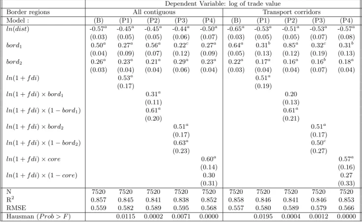
Table 3: The average trade-expanding impact of FDI on pooled flows

Dependent Variable: log of trade value

Border regions All contiguous Transport corridors

Model : (B) (P1) (P2) (P3) (P4) (B) (P1) (P2) (P3) (P4) ln(dist) -0.57a _-0.45a _-0.45a _-0.44a _-0.50a _-0.65a _-0.53a _-0.51a _-0.53a _-0.57a (0.03) (0.05) (0.05) (0.06) (0.07) (0.03) (0.05) (0.05) (0.07) (0.08) bord1 0.50a 0.27a 0.56a 0.22c 0.27a 0.64a 0.31b 0.85a 0.32c 0.31b (0.04) (0.09) (0.07) (0.12) (0.09) (0.05) (0.13) (0.12) (0.19) (0.13) bord2 0.26a 0.23a 0.21a 0.29a 0.23a 0.22a 0.17a 0.16a 0.16b 0.18a (0.03) (0.04) (0.04) (0.06) (0.04) (0.03) (0.04) (0.04) (0.07) (0.04) ln(1 + f di) 0.53a _0.51a (0.17) (0.19) ln(1 + f di) × bord1 0.31a 0.20 (0.11) (0.13) ln(1 + f di) × (1 − bord1) 0.61a 0.61a (0.20) (0.21) ln(1 + f di) × bord2 0.51a 0.51a (0.17) (0.17) ln(1 + f di) × (1 − bord2) 0.63a 0.50c (0.23) (0.27) ln(1 + f di) × core 0.60a _0.57a (0.14) (0.16) ln(1 + f di) × (1 − core) 0.30 0.27 (0.31) (0.33) N 7520 7520 7520 7520 7520 7520 7520 7520 7520 7520 R2 _{0.857 0.845 0.841 0.838 0.852 0.858 0.846 0.841 0.846 0.853} RMSE 0.559 0.582 0.589 0.595 0.568 0.557 0.580 0.589 0.579 0.566 Hausman (P rob > F ) 0.0115 0.0002 0.0071 0.0000 0.0195 0.0004 0.0012 0.0000 Note: Heteroskedasticity-robust standard errors in brackets, with a_, b _and c _{denoting significance at the 1%, 5%}

and 10% levels, respectively. Fixed-effects are not reported. “Hausman” provides the p-value of the Fisher test for significance of dξiJtin structural equation (9). A p-value < 0.05 means that the null of the FDI exogeneity is rejected

border region dummy, in order to disentangle its marginal impact between border and interior regions. In the same spirit, column (P4) interacts FDI with a core border region dummy (defined independently of the partner country),18_{so as to assess whether trade differentials exist due to the presence of foreign}

affiliates either from the nearby country, or from the other countries in the sample. Table 4 reports similar results for the sample of respectively exports (columns (X1), (X2), (X3) and (X4)) and imports (columns (M1), (M2), (M3) and (M4)).

As can be seen in Table 3, there is a strong positive relationship between inward multinational activity and trade. A 10% increase in the foreign stock of affiliates entails a 5.3% increase in trade with the parent country. This net complementarity is significantly larger for exports (8%) than for imports (2.6%), which casts doubt on the existence of a bias in consumers’s preferences that would be conveyed by the FDI channel. As the α estimates are not significantly different from 0 in most import specifications, this could be evidence that border regions are mostly export platforms towards nearby countries. In most of the estimations, we cannot reject the null of exogeneity of FDI at the 5% significance level, which means that 2SLS are consistent estimators. Incidentally, in all the first-stage regressions, the stock of FDI is actually partially correlated with our market potential variable, which makes us confident in the validity of this instrument.19

More importantly, we see that augmenting the gravity specification with FDI greatly reduces the coefficients of the bord1 variable. For the border regions defined according to a strict

contigu-ity criterion, the deviation from the gravcontigu-ity norm falls from 64.9% ([exp(0.50) − 1] × 100) to 31% ([exp(0.27) − 1] × 100), whereas transport corridors face a similar fall in their lead place, from 89.6% ([exp(0.64) − 1] × 100) to 36.3% ([exp(0.31) − 1] × 100). Present FDI in the gravity specification, transport corridors do not longer outperform regarding exports. Therefore, nearly half of the trade outperformance of first-order border regions is actually due to the presence of foreign affiliates from the nearby country.20 However, the elasticity of trade with respect to FDI is actually significantly larger within the group of interior regions (0.61) than within that of first-order border regions (either 0.31 or 0.20 depending on their subjacent definition). Nonetheless, we have to bear in mind that the regions who share a frontier with a country host, on average, around 14 times more affiliates from this country than interior regions. Therefore, although the trade-expanding effect of each additional affiliate is larger for interior than for border regions, this is compatible with an average trade-creating impact of FDI larger for the former than for the latter.

18_{Which means that “core” is a dummy taking the value 1 whenever trade observed relates to a region located at the}

Belgium-Luxembourg or at the German borders (whatever trade concerns these countries or not). See Appendix B for a precise listing of these regions.

T able 4: The av erage trade-expanding impact of FDI on either imp orts or exp orts Dep enden t V ariable: log flo w Border regions All con tiguous T ransp ort corridors Mo del : (X1) (M1) (X2) (M2) (X3) (M3) (X4) (M4) (X1) (M1) (X2) (M2) (X3) (M3) (X4) (M4) ln (dist ) -0.28 a -0.62 a -0.28 a -0.62 a -0.25 b -0.62 a -0.28 b -0.71 a -0.30 a -0.75 a -0.29 a -0.73 a -0.28 b -0.78 a -0.29 b -0.86 a (0.08) (0.06) (0.08) (0.06) (0.10) (0.07) (0.11) (0.09) (0.08) (0.06) (0.09) (0.07) (0.11) (0.08) (0.13) (0.11) bor d1 -0.04 0.58 a 0.27 a 0.84 a -0.13 0.57 a -0.04 0.58 a -0.12 0.75 a 0.37 a 1.33 a -0.21 0.85 a -0.12 0.74 a (0.13) (0.11) (0.08) (0.13) (0.18) (0.15) (0.13) (0.12) (0.20) (0.17) (0.11) (0.25) (0.31) (0.25) (0.20) (0.19) bor d2 0.15 a 0.30 a 0.14 a 0.29 a 0.26 a 0.31 a 0.15 a 0.31 a 0.07 0.27 a 0.06 0.26 a 0.14 0.18 b 0.06 0.29 a (0.05) (0.05) (0.05) (0.05) (0.08) (0.07) (0.05) (0.05) (0.06) (0.05) (0.06) (0.05) (0.10) (0.09) (0.07) (0.06) ln (1 + f di ) 0.80 a 0.26 0.88 a 0.14 (0.27) (0.21) (0.30) (0.22) ln (1 + f di ) × bor d1 0.57 a 0.06 0.60 a -0.19 (0.16) (0.15) (0.19) (0.19) ln (1 + f di ) × (1 − bor d1 ) 0.88 a 0.33 0.97 a 0.24 (0.30) (0.24) (0.34) (0.26) ln (1 + f di ) × bor d2 0.76 a 0.25 0.86 a 0.16 (0.28) (0.20) (0.30) (0.21) ln (1 + f di ) × (1 − bor d2 ) 0.98 a 0.29 1.00 b 0.00 (0.37) (0.27) (0.46) (0.33) ln (1 + f di ) × cor e 0.79 a 0.41 b 0.87 a 0.26 (0.21) (0.18) (0.26) (0.21) ln (1 + f di ) × (1 − cor e) 0.81 c -0.22 0.94 c -0.41 (0.48) (0.40) (0.55) (0.45) N 3760 3760 3760 3760 3760 3760 3760 3760 3760 3760 3760 3760 3760 3760 3760 3760 R 2 0.844 0.909 0.837 0.907 0.818 0.909 0.842 0.901 0.830 0.911 0.823 0.908 0.812 0.909 0.822 0.891 RMSE 0.561 0.508 0.572 0.515 0.606 0.510 0.564 0.533 0.585 0.505 0.598 0.512 0. 615 0.509 0.598 0.556 Hausman (P rob > F ) 0.0002 0.6140 0.0007 0.0057 0.0005 0.3218 0.0000 0.0000 0.0001 0.9949 0.0004 0.0053 0.0000 0.1427 0.0000 0.0000 Note: Heterosk edasticit y-robust standard errors in brac kets, with a , b and c denoting significance at the 1%, 5% and 10% lev els, resp ectiv ely . Fixed-effects are not rep orted. “Hausman” pro vides the p-v alue of the Fisher test for significance of d ξiJ t in structural equations (9 ). A p-v alue < 0. 05 means that the n ull of the FDI exogeneit y is rejected at the 5% significance lev el.

By disentangling further the effect of FDI within two additional groups, we see that not only core border regions benefit from a larger FDI trade-creating impact on average, but also at the margin. Indeed, the α coefficient is larger within the group of core regions (around 0.6) than elsewhere (around 0.3, but insignificant).

Finally, the distance coefficients also reduce consequently to the inclusion of FDI into the gravity specification. Hence, distance actually captures other effects than spatial proximity, and merely effects conveyed by variables that are negatively correlated with FDI, such as tariffs, information or jurisdiction costs. Therefore, spatial proximity matters for trade, but in a quite complex way that goes beyond the impact of shipment costs or “physical” geography.

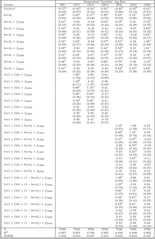
Tables 5 and 6 provide further insights regarding the trade dynamics observed on the period 1993-2000. The main explanatory variables are thus interacted with year dummies in order to show the time trends experienced by their coefficients. As previously, in Table 5, column (B) reports the results of estimating equation (9) (excluding FDI from the specification) on the 1993-2000 sub-sample of pooled flows. Columns (P1), (X1) and (M1) provide the 2SLS estimates of structural equation (12) for respectively the pooled, exports and import flows, whereas columns (P2), (X2) and (M2) (respectively (P4), (X4) and (M4) in Table 6) disentangles the marginal impact of FDI within the group of border and interior regions .

Column (P1) in Table 5 shows that, once controlled for inward FDI, the trade outperformance of border regions is drastically reduced: the positive trade deviation from the gravity norm falls and becomes insignificant for nearly all the period 1993-2000. Furthermore, the trade-creating effect of inward FDI diminishes in magnitude (it is divided by nearly 7 from 1993 to 2000), and loses significance over time, until becoming insignificant for the most recent years of observation. This could indicate an increasing orientation of foreign firms towards the French market. Over time, foreign affiliates both sell more to French consumers or firms and buy more from French suppliers, and hence, reduce their trade with the origin country. However, this effect is not sufficiently strong to eliminate the trade creating impact of FDI over the whole period 1993-2000. Even though horizontal motives seem to become prevalent over time, overall, FDI appears as a complement rather than a substitute for trade. The erosion of the trade expanding impact of foreign affiliates is lower for interior than border regions, the FDI elasticity being divided by 5.5 on the same period. Therefore, decreasing returns to scale in the benefits of FDI seem to prevail over the period 1993-2000.

level. Related results are available upon request.

Table 5: Time changes in the average trade-expanding impact of FDI Dependent Variable: log flow

Model : (B) (P1) (X1) (M1) (P2) (X2) (M2) ln(dist) -0.57a _-0.42a _-0.24c _-0.61a _-0.43a _-0.25b _-0.61a (0.03) (0.07) (0.13) (0.07) (0.06) (0.10) (0.07) bord2 0.26a 0.23a 0.17a 0.30a 0.22a 0.16a 0.29a (0.03) (0.04) (0.06) (0.05) (0.04) (0.06) (0.05) bord1× f1993 0.54a 0.23 -0.18 0.64a 0.53b 0.31 0.74b (0.10) (0.25) (0.52) (0.24) (0.24) (0.38) (0.37) bord1× f1994 0.53a 0.01 -0.42 0.44 0.35 0.07 0.63b (0.09) (0.31) (0.59) (0.31) (0.22) (0.35) (0.32) bord1× f1995 0.50a 0.25 -0.15 0.65a 0.41 -0.02 0.85c (0.09) (0.20) (0.35) (0.25) (0.25) (0.26) (0.51) bord1× f1996 0.52a 0.32c -0.04 0.67a 0.61b 0.20 1.02c (0.09) (0.17) (0.26) (0.24) (0.28) (0.18) (0.58) bord1× f1997 0.49a 0.23 0.03 0.43c 0.58b 0.15 1.01c (0.09) (0.18) (0.24) (0.26) (0.27) (0.18) (0.58) bord1× f1998 0.51a 0.32c 0.07 0.57b 0.70b 0.30 1.10c (0.09) (0.19) (0.26) (0.27) (0.27) (0.20) (0.57) bord1× f1999 0.48a 0.33 0.07 0.60c 0.70a 0.30 1.10b (0.09) (0.22) (0.28) (0.31) (0.26) (0.19) (0.52) bord1× f2000 0.45a 0.33 0.18 0.49 0.59b 0.55b 0.62c (0.08) (0.22) (0.29) (0.30) (0.23) (0.26) (0.36) ln(1 + f di) × f1993 1.90c 3.00 0.81 (1.02) (2.13) (0.89) ln(1 + f di) × f1994 1.53b 2.16 0.90 (0.71) (1.37) (0.69) ln(1 + f di) × f1995 0.68c 1.16c 0.21 (0.38) (0.67) (0.41) ln(1 + f di) × f1996 0.48c 0.82c 0.13 (0.26) (0.43) (0.31) ln(1 + f di) × f1997 0.52b 0.63c 0.41 (0.25) (0.38) (0.31) ln(1 + f di) × f1998 0.41 0.58 0.24 (0.25) (0.39) (0.31) ln(1 + f di) × f1999 0.35 0.50 0.20 (0.29) (0.42) (0.35) ln(1 + f di) × f2000 0.30 0.41 0.19 (0.29) (0.41) (0.37) ln(1 + f di) × bord1× f1993 1.10c 1.68 0.53 (0.65) (1.29) (0.71) ln(1 + f di) × bord1× f1994 0.98b 1.37c 0.59 (0.40) (0.76) (0.42) ln(1 + f di) × bord1× f1995 0.47c 0.97b -0.04 (0.28) (0.39) (0.52) ln(1 + f di) × bord1× f1996 0.20 0.59a -0.18 (0.23) (0.23) (0.45) ln(1 + f di) × bord1× f1997 0.24 0.52a -0.04 (0.21) (0.19) (0.42) ln(1 + f di) × bord1× f1998 0.15 0.41b -0.11 (0.20) (0.21) (0.36) ln(1 + f di) × bord1× f1999 0.14 0.35 -0.07 (0.20) (0.22) (0.34) ln(1 + f di) × bord1× f2000 0.16 0.21 0.12 (0.21) (0.27) (0.29) ln(1 + f di) × (1 − bord1) × f1993 1.88b 2.96 0.81 (0.93) (1.86) (0.86) ln(1 + f di) × (1 − bord1) × f1994 1.55b 2.18 0.92 (0.70) (1.34) (0.70) ln(1 + f di) × (1 − bord1) × f1995 0.66c 1.12c 0.20 (0.35) (0.61) (0.40) ln(1 + f di) × (1 − bord1) × f1996 0.48c 0.81b 0.15 (0.26) (0.41) (0.32) ln(1 + f di) × (1 − bord1) × f1997 0.53b 0.61c 0.44 (0.25) (0.36) (0.33) ln(1 + f di) × (1 − bord1) × f1998 0.44 0.58 0.31 (0.27) (0.40) (0.35) ln(1 + f di) × (1 − bord1) × f1999 0.41 0.53 0.30 (0.34) (0.47) (0.44) ln(1 + f di) × (1 − bord1) × f2000 0.34 0.46 0.22 (0.33) (0.46) (0.43) N 7520 7520 3760 3760 7520 3760 3760 R2 0.857 0.827 0.793 0.905 0.830 0.808 0.903 RMSE 0.559 0.615 0.647 0.521 0.610 0.623 0.527

Note: Heteroskedasticity-robust standard errors in brackets, witha_,b _andc

Table 6: Time changes in the average trade-expanding impact of FDI in core regions

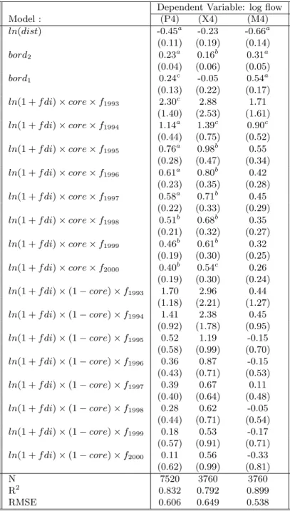
Dependent Variable: log flow

Model : (P4) (X4) (M4) ln(dist) -0.45a _{-0.23 -0.66}a (0.11) (0.19) (0.14) bord2 0.23a 0.16b 0.31a (0.04) (0.06) (0.05) bord1 0.24c -0.05 0.54a (0.13) (0.22) (0.17) ln(1 + f di) × core × f1993 2.30c 2.88 1.71 (1.40) (2.53) (1.61) ln(1 + f di) × core × f1994 1.14a 1.39c 0.90c (0.44) (0.75) (0.52) ln(1 + f di) × core × f1995 0.76a 0.98b 0.55 (0.28) (0.47) (0.34) ln(1 + f di) × core × f1996 0.61a 0.80b 0.42 (0.23) (0.35) (0.28) ln(1 + f di) × core × f1997 0.58a 0.71b 0.45 (0.22) (0.33) (0.29) ln(1 + f di) × core × f1998 0.51b 0.68b 0.35 (0.21) (0.32) (0.27) ln(1 + f di) × core × f1999 0.46b 0.61b 0.32 (0.19) (0.30) (0.25) ln(1 + f di) × core × f2000 0.40b 0.54c 0.26 (0.19) (0.30) (0.24) ln(1 + f di) × (1 − core) × f1993 1.70 2.96 0.44 (1.18) (2.21) (1.27) ln(1 + f di) × (1 − core) × f1994 1.41 2.38 0.45 (0.92) (1.78) (0.95) ln(1 + f di) × (1 − core) × f1995 0.52 1.19 -0.15 (0.58) (0.99) (0.70) ln(1 + f di) × (1 − core) × f1996 0.36 0.87 -0.15 (0.43) (0.71) (0.53) ln(1 + f di) × (1 − core) × f1997 0.39 0.67 0.11 (0.40) (0.64) (0.48) ln(1 + f di) × (1 − core) × f1998 0.28 0.62 -0.05 (0.44) (0.71) (0.54) ln(1 + f di) × (1 − core) × f1999 0.18 0.53 -0.17 (0.57) (0.91) (0.71) ln(1 + f di) × (1 − core) × f2000 0.11 0.56 -0.33 (0.62) (0.99) (0.81) N 7520 3760 3760 R2 _{0.832 0.792 0.899} RMSE 0.606 0.649 0.538

Note: Heteroskedasticity-robust standard errors in brackets, with a_, b _and c _{denoting significance at the 1%, 5% and 10%}

Because interior regions were initially less attractive than border regions, the decline experienced in the gains arising from attracting new affiliates could be less pronounced for the former than for the latter.

As can be seen in Table 6, even though core border regions experience a similar fall in FDI trade-expanding gains throughout the period, the erosion is also less dramatic there and, most importantly, the trade outperformance remains highly significant at the end of the period. A plausible explanation for the drastic fall in trade outperformances suffered by the French border regions located at the periphery of Europe would be that, during the period 1978-2000, they did not benefit from any major cross-border transport developments, whereas their communications with the north of France (in the form of new highways and railroad infrastructure) improved notably. Hence, the trade orientation of these regions shifted from their neighboring countries (Spain and Italy) towards the French northern market that was becoming more accessible overtime.

5

Conclusion

In this paper we have used an augmented gravity model to explain the geography of trade within France, over the period 1978-2000. Firstly, we have compared the trade performances of 94 regions according to their geographic position “vis-`a-vis” a bloc of five neighboring countries of France, during their ongoing process of integration within Europe. We find that the regions sharing a frontier with a country trade on average as much as 70% more with this partner than other regions, once controlled for the own region-specific and country-specific characteristics. As European integration progressed, the French border regions located at the vicinity of the EU core succeeded in triggering new trade surpluses, whereas those located at the western periphery of Europe did not. Even though temporary gains were drawn from integration shocks such as the Single European Act, the Schengen Agreement and the Maastricht Treaty, they were not sufficient to counteract the drastic long-term decline suffered by the southern French regions bordering Spain and Italy.

Secondly, we have assessed how much of the observed trade differentials can be explained by the location strategy of foreign affiliates from the five countries studied. The spatial distribution of inward FDI across French regions, as its post-integration changes, explain partly these differentials. We find that inward FDI is on average trade-expanding, independently of both the country source and the geographic position of regions. Recalling that trade and outsourcing are complements whereas horizontal FDI is clearly a substitute for trade, this could be evidence that FDI from French bordering countries are mostly vertically motivated. The magnitude of the induced overtrade is larger for border regions than for their interior counterparts. However, the marginal effect of FDI is stronger for interior