HAL Id: halshs-00676500
https://halshs.archives-ouvertes.fr/halshs-00676500
Preprint submitted on 5 Mar 2012
HAL is a multi-disciplinary open access
archive for the deposit and dissemination of
sci-entific research documents, whether they are
pub-lished or not. The documents may come from
teaching and research institutions in France or
L’archive ouverte pluridisciplinaire HAL, est
destinée au dépôt et à la diffusion de documents
scientifiques de niveau recherche, publiés ou non,
émanant des établissements d’enseignement et de
recherche français ou étrangers, des laboratoires
Optimal Lifecycle Fertility in a Barro Becker Economy
Pierre Pestieau, Grégory Ponthière
To cite this version:
Pierre Pestieau, Grégory Ponthière. Optimal Lifecycle Fertility in a Barro Becker Economy. 2012.
�halshs-00676500�
WORKING PAPER N° 2012 – 11
Optimal Lifecycle Fertility in a Barro Becker Economy
Pierre Pestieau
Grégory Ponthière
JEL Codes: D10, J13, O40
Keywords: Fertility, Birth Timing, Population, Dynastic Altruism, OLG Model
P
ARIS
-
JOURDAN
S
CIENCES
E
CONOMIQUES
48, BD JOURDAN – E.N.S. – 75014 PARIS
TÉL. : 33(0) 1 43 13 63 00 – FAX : 33 (0) 1 43 13 63 10
Optimal Lifecycle Fertility in a Barro-Becker
Economy
Pierre Pestieau
yand Gregory Ponthiere
zMarch 5, 2012
Abstract
Parenthood postponement is a key demographic trend of the last three decades. In order to rationalize that stylized fact, we extend the canonical model by Barro and Becker (1989) to include two instead of one -reproduction periods. We examine how the cost structure of early and late children in terms of time and goods a¤ects the optimal fertility tim-ing. Then, focusing a stationary equilibrium with stationary population, we provide two alternative explanations for the observed postponement of births: (1) a fall of the direct cost of late children (thanks to medical advances); (2) a rise in hourly productivity, which increases the (relative) opportunity costs of early children in comparison to late children.
Keywords: fertility, birth timing, population, dynastic altruism, OLG model.
JEL classi…cation codes: D10, J13, O40.
The authors are most grateful to David de la Croix for his helpful comments on this manuscript.
yUniversity of Liege, CORE, PSE and CEPR.
zEcole Normale Superieure, Paris, and Paris School of Economics. [corresponding author] Address: Ecole Normale Superieure, 48 boulevard Jourdan, 75014 Paris, France. E-mail: [email protected] Tel: 0033-143136204.
1
Introduction
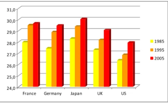
As this is well-known among demographers, human fertility has exhibited a globally decreasing pattern during the last century. At the world’s level, the total fertility rate (TFR) has decreased from about 5.2 children per women in 1900 to about 2.7 children per women in 2000.1 Another well documented stylized fact concerns not the number, but the timing of births: there has been, over the last three decades, a global tendency towards the postponement of parenthood. That stylized fact is illustrated by Figure 1, which shows the rise in the mean age at motherhood in several advanced economies, over 1985-2005.2
24,0 25,0 26,0 27,0 28,0 29,0 30,0 31,0
France Germany Japan UK US
1985 1995 2005
Figure 1: Mean age at motherhood (years), 1985-2005.
Another way to illustrate the postponement of births consists of decomposing the total fertility rate into the average number of children per women in the early part of the reproduction period (i.e. between ages 15 and 34 years), and the average number of children per women in the late part of the reproduction period (i.e. between ages 35 and 49 years).3 As shown on Figure 2, whereas the total fertility rate has remained relatively constant over the period 1985-2005, late fertility has signi…cantly increased over time. For instance, whereas children born from a mother older than 35 years amounted to only 7.5 percents of US births in 1985, that proportion jumped to about 14 percents in 2005.
Can economic models of fertility, such as the Barro Becker (1989) framework, provide some plausible explanation or rationalization of that stylized fact?4 At …rst glance, the answer seems to be negative, since that model includes, as most dynamic models with endogenous fertility, a unique reproduction period. However, that model can be extended, so as to introduce several reproduction periods, instead of a single one.
1The total fertility rate measures the average number of children a woman has on her lifecycle, while assuming that she survives during the entire reproduction period, and faces age-speci…c fertility rates during the whole reproduction period. The data are from Lee (2003).
2Data source: United Nations Population Division/DESA (2012). 3Data source: United Nations Population Division/DESA (2012).
4On the empirical side, see the studies by Schultz (1985), Heckman and Walker (1990), Ermisch and Ogawa (1994), Joshi (2002).
0 0,5 1 1,5 2 2,5 1985 1995 2005 1985 1995 2005 1985 1995 2005 1985 1995 2005 1985 1995 2005
France Germany Japan UK US
TFR > 35 TFR < 35
Figure 2: Decomposition of the total fertility rate (before and after 35 years), 1985-2005.
The goal of this paper is precisely to provide such an extension of the Barro Becker (1989) model. For that purpose, we keep the fundamental structure of the Barro Becker model: overlapping generations, physical capital accumulation, dynastic altruism, but we add one reproduction period, in such a way as to be able to examine whether the observed postponement of births can or cannot be rationalized by an economy à la Barro and Becker. Given that we are here only interested in the timing of fertility, we will, when discussing how to rationalize the postponement of births, assume that the total fertility rate equals the replacement level, and study the lifecycle distribution of births.5
Anticipating on our results, we …rst show that, at the temporary equilibrium, the cost structure of early and late children, in terms of goods and time, is a key determinant of the optimal fertility pro…le. If late children are more costly than early children during their childhood, and if early children are no longer time-consuming once adult, the optimal fertility pro…le only involves early children. If, however, early children are, once adult, still time-consuming for their par-ents, that additional opportunity cost provides some incentive for postponing fertility. Then, focusing on a stationary equilibrium with stationary population size, we show that improvements in total factor productivity tend, under gen-eral conditions, to shift steady-state optimal fertility pro…les towards more late births. Hence the extended Barro Becker model proposes two explanations for the postponement of births: either a change in the direct cost of early and late children, or, alternatively, a rise in total factor productivity.
In sum, the extended Barro Becker model is shown to be able to rationalize the observed postponement of births. As such, that model complements all static frameworks studying the optimal timing of births (Happel et al 1984, Cigno and Ermisch 1989, Gusta¤son 2001), as well as dynamic frameworks also focusing on lifecycle fertility patterns, but using alternative assumptions, such
5That stationary population assumption, which allows us to focus only on the birth timing problem, is actually quite plausible given the …niteness of the Earth. One could hardly imagine an ever growing population living on a …xed space.
as D’Albis et al (2010) and Pestieau and Ponthiere (2011).6
The rest of the paper is organized as follows. Section 2 presents the model. Section 3 studies lifecycle fertility at the temporary equilibrium. Section 4 exam-ines the timing of births at a stationary equilibrium with stationary population. Empirical material on total factor productivity and fertility timing in the U.S. and the OECD is studied in Section 5. Section 6 concludes.
2
The model
Let us consider a three-period OLG model. The three periods are: childhood, young adulthood and old adulthood. Agents work the entire time-period in young adulthood and old adulthood. Reproduction is monosexual. Agents can have children either at the beginning of young adulthood (i.e. second period), or at the beginning of old adulthood (i.e. third period). The number of early children for a young adult at time t is denoted by nt, while the number of late children for a young adult at time t is denoted by mt+1.
Following Barro and Becker (1989), we assume that parents are altruistic towards young family members. Parents’utility depends on own consumption at young adulthood (denoted by ct) and at old adulthood (denoted by dt+1), and on the number and the utility of younger family members. The utility of an agent who is a young adult at time t is represented by the utility function:
Ut= v(ct) + v(dt+1) + a (Nt+1; Nt) Nt+1Ut+1 (1) where v( ) is the utility from consumption, is a time-preference factor, and the weighting function a( ) represents the weight assigned by a young adult belonging to the adult cohort at period t, of size Nt, to the welfare of each family member belonging to the adult cohort t + 1, of size Nt+1. The number of young adults at time t + 1, Nt+1, includes his own children, whose number is Ntnt, as well as the late children of his parents, i.e. his young brothers and sisters, whose number is Nt 1mt. Thus the number of family members who are young adults at time t > 0 is denoted by Nt+1= Ntnt+ Nt 1mt.7 That number of descendants can also be rewritten as:
Nt+1= Nt nt+ Nt 1mt Nt = Nt nt+ mt gt = Ntgt+1 (2) where gt+1 NNt+1t is the (adult) cohort growth factor, equal to nt+mgtt.
The family weighting function a( ) has the following form: a(Nt+1; Nt) =
Nt1 "Nt+1"
(3)
6D’Albis et al (2010) focus on optimal lifecycle fertility in a continuous time OLG model, under the assumption of a decreasing relationship between the total number of children and the timing of births. Pestieau and Ponthiere (2011) focus on the optimal fertility timing in an OLG model à la Samuelson (1976), and examine whether the Serendipity Theorem still holds in a broader demographic environment with several reproduction periods instead of one.
7We assume, to avoid any period without births, that N
where 0 < < 1 and 0 < " < 1. That functional form is a generalization of the one in Barro and Becker (1989), where gt+1= nt (as mt= 0).8 Note also that substituting for a(Nt+1; Nt) in expression (1) yields:
Ut= v(ct) + v(dt+1) + (gt+1)1 "Ut+1 (4) That expression generalizes the utility function used in Barro and Becker (1989), where all children are born from young parents (i.e. gt+1= nt), yielding:
Ut= v(ct) + v(dt+1) + (nt)1 "Ut+1 (5) In the Barro Becker setting, the unique fertility rate ntserves as the investment rate in the future. Here, in our framework with two reproduction periods, that investment rate in the future equals gt+1 nt+mgtt.
Substituting repeatedly for a cohort’s utility in the utility function of the dynastic head, we obtain the following dynastic utility function:
U0= 1 X t=0 t(N t)1 "[v(ct) + v(dt+1)] (6)
That expression collapses to Barro and Becker’s standard dynastic utility func-tion when old adulthood does not matter ( = 0) and when there are no births in third period, i.e. mt= 0 for all t, in which case Nt= Nt 1nt 1=
t 1Y
s=0 ns.9 The dynastic head treats equally the welfare of two descendants born at the same point in time, even though one is related to him through a lower number of family ties than the other. The underlying intuition is that, even though there may be di¤erences, in the short-term, between grand children and grand-grand-grand children, those di¤erences appear minor once the dynasty includes a su¢ ciently large number of generations.
The elasticity of v ( ) with respect to consumption is assumed to be constant:
v(ct) = ct (7)
where < 1. That assumption is also made in Barro Becker (1989).
8Indeed, in Barro-Becker, we have Nt+1 = ntNt, so that a( ) = =hN1 " t n"tNt" i = =Ntn"t, implying a ( ) Nt+1 = g 1 " t+1 = n 1 "
t . Here that formula is generalized, to ob-tain a ( ) Nt+1= gt+11 "even when gt+16= ntas a consequence of mt> 0.
9Note that the above dynastic utility function keeps the standard properties of the one derived by Barro and Becker (1989). If one had used, instead of expression (1), another utility function, such as, for instance:
Ut= v(ct) + v(dt+1) + a(nt)ntUt+1+ a(mt+1)mt+1Ut+2
with a( ) concave in its argument, one would not have been able to derive a dynastic utility function with the same simple form as expression (6). Indeed, the altruistic weighting function is non linear, so that a (n0n1) + a(m1) 6= a(n0n1+ m1), implying that the dynastic utility function can hardly be reduced to an in…nite sum of lifetime welfare terms weighted by the (concavi…ed) size of the di¤erent successive cohorts, as in Barro Becker (1989) and in (6).
Each adult earns a wage wton time supplied to the market, in young adult-hood and old adultadult-hood. Since we de…ne an adult’s total time available per period to be 1 unit, wt and wt+1 denote the total labour income in, respec-tively, young adulthood and old adulthood, in the case of no children.
Following Barro and Becker (1989), we assume that a child costs, during his childhood, a fraction b of the time unit of parents, so that parents having nt children can only work during a period 1 bntat young adulthood. Similarly, parents who have mt+1late children can only work a fraction 1 Bmt+1of their second working period. It is widely documented that a late child is more costly than an early child, so that we have: B b.10
However, the duration of coexistence of the parent with a child is longer with an early child than with a late child, and this may induce some additional time costs at older adulthood. We represent those extra time costs by the fraction h 0. The intuition is that early children are not only "enjoyed" longer than late children, but they also require some time once they are young adults. The source of asymmetry in comparison with late children is that late children become adults when their parents are retired, unlike early children, who become adults when their parents are still working. This di¤erence creates an asymmetry in the lifetime opportunity costs of early and late children.
Within the Barro-Becker (1989) setting, there is only one adult life-period. As a consequence, there is no savings: the only way to transfer resources over time is through bequests to children, each adult parent giving, in the last period of his life, a bequest to his children. Here, on the contrary, adulthood includes two periods, during which the agents works and can have children. The intro-duction of an additional life-period tends to complicate the analysis. Hence, we will make here three assumptions, which insure analytical solvability:
Young individuals can save resources for the future.11
All children, whatever these are born from young or old parents, receive their bequests at the same point in their lifetime, that is, at the beginning of young adulthood (i.e. the majority age).12
All children who live in the same time period receive exactly the same bequest from their parents, whatever those parents are young or old.13 Under those assumptions, a young adult at time t, whatever he is born from
1 0On the cost di¤erential between early and late children, see Gustafsson (2001).
1 1The introduction of savings allows us to characterize the agent’s intertemporal budget constraint even if he has no children early in life.
1 2One can interpret this as parental will to give an equal chance to all children, early and late. On the analytical side, that assumption helps a lot. If children received their bequests at the time of the death of their parent, then their lifetime budget constraint would di¤er, depending on whether they are born from young or old parents (see below).
1 3According to that assumption, only the timing of life determines the bequest one receives, and not the age of parents. The underlying idea is that, from the point of view of the dynastic head, a late child and an early grand child are similar, since they are alive at the same point in time, and, thus, equally "distant" from the dynastic head.
young or old parents, faces the budget constraint:
wt(1 bnt) + (1 + rt)kt= ct+ st+ ntet+ ntkt+1 (8) where (1 + rt)ktis the bequest received by the young adult from his parent, stis savings, etis the cost of an early child in terms of resources, b is the fraction of time dedicated to the rearing of each early child, and ntkt+1are the resources he saves to provide a bequest to his early children. The amount ntkt+1 is invested in the production process, and then given, with interests, to the children born at t once these are adults. Thus each of those children receives: (1 + rt+1)kt+1. At the next period, the adult agent faces the budget constraint:
wt+1(1 Bmt+1 hnt) + st(1 + rt+1) = dt+1+ mt+1Et+1+ mt+1kt+2 (9) where Et+1 is the cost of a late child in terms of resources, B is the fraction of time dedicated to each late child, and h is the fraction of time dedicated to early children once adults. Given that the cost of a late child is generally larger than the cost of an early child, the assumption Et et is reasonable.14 The amount mt+1kt+2 constitutes the resources that the parent saves to provide a bequest to his late children. The amount mt+1kt+2is invested in the production process, and then given, with interests, to the children born at t + 1 once these are adults. Each of those late children receives: (1 + rt+2)kt+2.
Substituting for savings in the young age budget constraint yields the indi-vidual’s intertemporal budget constraint:
wt(1 bnt) + wt+1(1 Bmt+1 hnt) 1 + rt+1 + (1 + rt)kt = ct+ ntet+ ntkt+1+ dt+1+ mt+1Et+1+ mt+1kt+2 1 + rt+1 (10) That intertemporal budget constraint is the same for all agents, whatever these are born from young or old parents. That result would not prevail if children received their bequests at the death of their parents.15
Substituting repeatedly for kt in the intertemporal budget constraint, we obtain the following dynastic budget constraint:
k0+ 1 X t=0 ztNt(1 bnt)wt+ 1 X t=1 ztNt 1(1 Bmt hnt 1)wt = 1 X t=0 zt Ntct+ Nt dt+1 1 + rt+1 + 1 X t=0 ztNtntet+ 1 X t=0 zt+1Ntmt+1Et+1(11)
1 4On the cost di¤erential between early and late children, see Gusta¤son (2001).
1 5If children received their bequest at the death of their parent, the overall budget con-straints of agents born at the same point in time would di¤er, depending on whether they are born from young or from old parents. Individuals born from old parents receiving the bequests earlier in their lifecycle, they bene…t, thanks to a larger opportunity set for savings, from more resources on the lifetime, ceteris paribus, than individuals born from young adults, who need to wait more to get the bequest. See the Appendix on this.
where zt = t Y s=0
1
(1+rs). That constraint states that the present value of all
resources (LHS) must be equal to the present value of all expenditures. In com-parison with the standard Barro-Becker setting, the LHS and the RHS di¤er by the presence of third-period consumption on the RHS, and, also, by the de…ni-tion of the number of descendants, Nt, equal here to Nt 1 nt 1+mtN1tN1t 2 .
3
Temporary equilibrium
The optimization problem faced by the dynastic head consists of maximizing utility U0subject to the dynastic budget constraint, subject to the initial assets k0, and subject to the initial young adult cohort size N0 = 1. Through that maximization problem, each agent takes as given the path of wage rates wtand of interest rates rt, and selects a path for consumption at the young age and old age for all descendants, c0, c1, c2, ::: and d1, d2, d3, :::, bequests per young adult, k1, k2, ::: and age-speci…c fertility rates, n0; n1; n2; ::: and m1; m2; m3; :::.16
The dynastic head’s problem can be written as follows: max ct;dt;nt;mt;kt 1 X t=0 t(N t)1 "[v(ct) + v(dt+1)] s.t. k0+ 1 X t=0 ztNt(1 bnt)wt+ 1 X t=1 ztNt 1(1 Bmt hnt 1)wt = 1 X t=0 zt Ntct+ Nt dt+1 1 + rt+1 + 1 X t=0 ztNtntet+ 1 X t=0 zt+1Ntmt+1Et+1 First-order condition for optimal consumption of a young adult at time t is:
t(N
t)1 " ct 1= ztNt
where is the Lagrange multiplier associated with the dynastic budget con-straint. The FOC for optimal old-age consumption at period t + 1 is:
t(N
t)1 " dt+11=
ztNt 1 + rt+1 Combining those two FOCs yields:
dt+1 ct
1
= (1 + rt+1) (12)
Combining the FOC for optimal consumption of a young adult at t + 1 with the FOC for optimal consumption of a young adult at t, we have:
ct ct+1 1 = 1 nt+ mt gt " 1 1 + rt+1 (13)
1 6Note that, since the ob jective function is time-consistent, the paths chosen by the dynastic head will also be chosen by any other following descendants facing the same problem.
Thus the intergenerational consumption pro…le is increasing in the parameter , and decreasing in the cohort growth factor gt= NNtt1 and in the interest rate. Similarly, for old-age consumption, we have:
dt dt+1 1 = 1 nt 1+ mt 1 gt 1 " 1 1 + rt+1 (14) Regarding the optimal demography, we know from the FOC for consumption that the optimal cohort growth factor gt+1 satis…es the condition:
gt+1= " (1 + rt+1) ct ct+1 1 #1" (15) The optimal cohort growth factor is increasing in parental altruism, and in the interest rate, but decreasing in the parameter ". If the interest rate is constant, and if the intergenerational consumption path is also invariant over time, the optimal cohort growth factor is also constant over time. But beyond those properties, that condition does not, on its own, su¢ ce to characterize, for any period, a unique optimal fertility pro…le (nt; mt), since various fertility pro…les (nt; mt) can bring the optimal cohort growth factor gt+1, as long as (nt; mt) is such that nt+mgtt = gt+1. Hence, to characterize the optimal fertility path, it is necessary to focus on the FOCs for optimal age-speci…c fertility.
Keeping in mind that the number of persons born at period t can be written as Nt= Nt 1gt= Nt 1 nt 1+mtN1tN1t 2 , the FOCs for the optimal nt and mtare, respectively: 1 X j=0 t+1+j(1 ")(N t+1+j) " @Nt+1+j @nt [v(ct+1+j) + v(dt+2+j)] = 1 X j=0 zt+1+j @Nt+1+j @nt ct+1+j+ dt+2+j 1 + rt+2+j + ztNtbwt+ zt+1Nthwt+1 + ztNtet+ 1 X j=0 zt+1+j @Nt+1+j @nt nt+1+jet+1+j + 1 X j=0 zt+1+j @Nt+1+j @nt mt+1+jEt+1+j 1 X j=0 zt+1+j @Nt+1+j @nt (1 bnt+1+j)wt+1+j 1 X j=0 zt+2+j @Nt+2+j @nt (1 Bmt+2+j hnt+1+j)wt+2+j (16)
1 X j=0 t+1+j(1 ")(N t+1+j) " @Nt+1+j @mt [v(ct+1+j) + v(dt+2+j)] = 1 X j=0 zt+1+j @Nt+1+j @mt ct+1+j+ dt+2+j 1 + rt+2+j + ztNt 1Bwt + ztNt 1Et+ 1 X j=0 zt+1+j @Nt+1+j @mt nt+1+jet+1+j + 1 X j=0 zt+1+j @Nt+1+j @mt mt+1+jEt+1+j 1 X j=0 zt+1+j @Nt+1+j @mt (1 bnt+1+j)wt+1+j 1 X j=0 zt+2+j @Nt+2+j @mt (1 Bmt+2+j hnt+1+j)wt+2+j (17)
Those two FOCs are almost identical, except that these depend on how respectively ntand mtin‡uence the number of individuals born at all subsequent periods t + 1; t + 2; :::. Although that e¤ect is complex - since any change in fertility is followed by changes in the number of descendants at all next generations -, the relationship Nt = Nt 1gt = Nt 1 nt 1+mtN1tN1t 2 can
help us to quantify the relative levels of the derivatives @Nt+1+j
@ni and
@Nt+1+j
@mi .
Lemma 1 The partial derivatives of the number of descendants with respect to early and late fertility satisfy the following equation, for all t, j > 0:
@Nt+1+j @nt = Nt Nt 1 @Nt+1+j @mt = gt @Nt+1+j @mt Proof. See the Appendix.
Thus whether the marginal e¤ect of a change in early fertility on the total number of descendants is superior or inferior to the marginal e¤ect of a change in late fertility depends on whether the population is growing or not, that is, on whether gt exceeds 1 or not. Substituting for this in the FOC for optimal mt,
and simplifying yields: 1 X j=0 t+1+j(1 ")(N t+1+j) " @Nt+1+j @nt [v(ct+1+j) + v(dt+2+j)] = 1 X j=0 zt+1+j @Nt+1+j @nt ct+1+j+ dt+2+j 1 + rt+2+j + ztNtBwt + ztNtEt+ 1 X j=0 zt+1+j @Nt+1+j @nt nt+1+jet+1+j + 1 X j=0 zt+1+j @Nt+1+j @nt mt+1+jEt+1+j 1 X j=0 zt+1+j @Nt+1+j @nt (1 bnt+1+j)wt+1+j 1 X j=0 zt+2+j @Nt+2+j @nt (1 Bmt+2+j hnt+1+j)wt+2+j (18)
That FOC can then be compared with the FOC for optimal nt. Several cases can arise, depending on the relative levels of early and late children in terms of time and goods.
Let us start with the simplest case. If there is perfect equality of all costs, i.e. b = B, et= Etand h = 0, then the two FOCs are exactly identical. Thus, in that special case, the optimal early fertility rate nt and late fertility rate are determined jointly, by the same condition. The dynastic head’s planning problem is thus underdetermined.
If, on the contrary, there is perfect equality of all costs, except that the early children still recommend some time at the adult age, i.e. h > 0. Then, it follows that the marginal welfare loss from increasing early fertility rate is always larger, ceteris paribus, than the marginal welfare loss from increasing the late fertility rate, since the RHS of the FOC for optimal nt always exceeds the one for optimal mt. We thus have the corner solution: nt= 0, mt> 0.
Alternatively, if there is no time costs of early children at the adult age (h = 0), but if late children have a larger cost, either in time or in goods, i.e. b B and et < Et or b < B and et Et, the marginal welfare loss from increasing early fertility is always smaller, ceteris paribus, than the marginal welfare loss from increasing late fertility, since the RHS of the FOC for optimal mtalways exceeds the one for optimal nt. Hence, we have: nt> 0 and mt= 0. Finally, when none of those conditions are satis…ed, the two FOCs are satis-…ed simultaneously, and we have the interior optimum for the fertility pro…le as a whole: nt> 0 and mt> 0. The following proposition summarizes our results. Proposition 1 If b B and et< Et or b < B and et Et, as well as
If b = B, et = Et and h > 0, the optimal fertility pro…le involves nt= 0 and mt> 0.
If b = B, et= Etand h = 0, the optimal fertility pro…le is indeterminate. Otherwise, the optimal fertility pro…le involves nt> 0 and mt> 0. Proof. See the above FOCs.
In sum, various fertility pro…les (nt; mt) can constitute the solution to the dynastic head’s optimization problem, depending on the structure of early and late children costs in terms of goods and in terms of time. Therefore, the evolution of children cost structure is likely to have had a signi…cant impact on the timing of births. One can think, for instance, that recent medical advances, such as the development of assisted reproductive technologies, have strongly reduced the cost of late children, leading to the observed postponement of births. However, as we shall now see, that kind of "cost-based explanation" is not the unique possible one. Other explanations can account for the postponement of births, without relying on external changes in children costs structure.
4
Births postponement: theory
In order to identify other potential determinants of the change in the timing of births, let us …rst make some additional assumptions, concerning the production process, from which wages wtand interest rates rtare determined. In this paper, we assume, like Barro and Becker (1989), a closed economy, where the wages and interest rates depend on the level of the stock of productive capital.
4.1
Production
Production takes place via a standard one-sector production function that ex-hibits constant returns to scale:
Yt= F (Kt; Lt) (19)
where Yt is total output, Kt is total capital, and Lt is total labour. As Barro Becker (1989), we assume no depreciation of physical capital.
The total labour at period t can be written as:
Lt = (1 bnt)Nt+ (1 Bmt hnt 1)Nt 1 = Nt 1 bnt+
1 Bmt hnt 1 gt
(20) The total capital stock at period t can be written as:
Kt= (Nt 1nt 1+ Nt 2mt 1) kt+ Nt 1st 1= Ntkt+ Nt
gt
where the …rst term of the RHS coincides with the bequest received by indi-viduals who are young adults at time t, whereas the second term is the savings from young adults at the previous period.
In intensive terms, we can denote the capital per worker tas:
t Kt (1 bnt)Nt+ (1 Bmt hnt 1)Nt 1 = kt+ st 1 gt 1 bnt+1 Bmtgthnt 1 (22)
Given constant returns to scale, we can rewrite the production process as: yt
Yt
(1 bnt)Nt+ (1 Bmt hnt 1)Nt 1
= F ( t; 1) = f ( t) (23) with, as usual, f0( t) > 0, f00( t) < 0.
Factors are assumed to be paid at their marginal productivities:
rt = f0( t) (24)
wt = f ( t) tf0( t) (25)
The interest rate is decreasing in t, while the wage rate is increasing in t.
4.2
Long-run fertility timing
The dynamics of our economy is quite complex, because there are not one, but three demographic variables: early fertility rate nt (like in Barro-Becker), but, also, late fertility rate mt, and the cohort growth factor gt= nt 1+mgtt11.
Hence, to facilitate our analysis of the change in fertility timing, we will here assume that there exists a unique stable stationary equilibrium with a station-ary population. That assumption can be justi…ed on the ground of analytical tractability, but, also, on the ground that an ever increasing or decreasing pop-ulation is hardly plausible on a …nite Earth. Moreover, in the light of Pestieau and Ponthiere (2011), it appears that, when the cohort growth factor g di¤ers from unity, stationary equilibria can, under some fertility pro…les, turn out to be unstable, making steady-state analysis irrelevant. Thus imposing a stationary population protects us against the possibility of unstable stationary equilibria, but without preventing the study of the optimal fertility timing.17
When there exists a stationary equilibrium, we know, since:
gt+1= " (1 + rt+1) ct ct+1 1 #1"
1 7On the existence and stability of a stationary equilibrium with exogenous age-speci…c fertility rates n and m, see Pestieau and Ponthiere (2011). It is shown there that, although there exists, under mild conditions, a stationary equilibrium in an OLG model with two reproduction periods, the stability of that equilibrium requires n > 0. When n = 0, the economy exhibits cyclical dynamics around a stationary equilibrium, except when g equals 1, in which case there is a stable stationary equilibrium.
that the cohort growth rate gt must be constant over time, and equal to: g = [ (1 + r( ))]1" (26)
Note that, for a given, constant, cohort growth factor g = 1, there exist various possible fertility pro…les (n; m). Indeed, any pair (n ; m ) such that:
1 = n +
2
p
n 2+ 4m 2
is compatible with the stationary equilibrium with stationary cohort size. To study the optimal fertility pro…le, let us go back to the conditions de-scribing the optimal levels of n and m , and substitute for steady-state wages, interest rate, and child costs. Making those substitutions in the two FOCs and substituting for the Lagrange multiplier in the …rst FOC by means of the other FOC, we obtain the optimality condition:
e + bw + hw
1 + r = E + Bw (27)
That condition is necessary for the two FOCs to be satis…ed, that is, for an interior optimal fertility pro…le with n > 0, m > 0. It states that the marginal cost from an early child (LHS), in terms of goods (1st term) or in time (2nd and 3rd terms), must be exactly equal to the marginal cost from a late child (RHS), in terms of goods (1st term) and time (2nd term). On its basis, we can characterize the steady-state fertility pro…le.
Proposition 2 Consider an economy with a unique stable stationary equilib-rium and a stationary population.
(i) if Bw + E > e + bw + hw 1+r , we have n = 1, m = 0; (ii) if Bw + E = e + bw + hw 1+r , we have n > 0, m > 0; (iii) if Bw + E < e + bw + hw 1+r , we have n = 0, m = 1: Proof. See the Appendix.
Proposition 2 allows us to propose a …rst explanation for the observed post-ponement of births. In the early stages of history, late children were extremely costly. Hence, the large levels of B and E push the economy towards case (i). However, as medical science has developed, the costs of late children have decreased substantially, pushing the economy towards case (ii), with interior optimal early and late fertility rates. But that stage may not be the end of the story: as the costs of late parenthood become closer and closer to those of early parenthood (i.e. B ! b and E ! e), the existence of a positive time cost for early children who become adults (i.e. h > 0) may push the economy towards case (iii), with a corner solution n = 0 and m = 1.
In sum, Proposition 2 proposes a cost-based explanation to the observed postponement of births. Over time, the structure of child costs would have
evolved, with, as a consequence, a shift from early fertility to late fertility. Note that, whereas the shift from stage (i) (no late births) to stage (ii) (mixed fertility) as a result of medical advances reducing late children costs E could have been anticipated a priori, the shift from stage (ii) to stage (iii) is less trivial. That shift relies on the fact that children are durable consumption goods, who also involve a durable opportunity cost. Thus the model has the virtue to highlight the key role played by that durable time costs of children for the optimal fertility timing issue.
Although attractive, that explanation is not the unique possible one. Actu-ally, we can also propose another explanation, which relies not on the structure of child costs, but on the evolution of the production process. To explore that explanation further, let us impose a particular functional form on the production process, i.e. the standard Cobb-Douglas production function:
Yt= AKtL 1
t (28)
where A > 0 is a productivity parameter, while is the elasticity of output with respect to capital. In intensive terms, the production process can be written as:
yt= A t (29)
Hence, at the stationary equilibrium with stationary population, the steady-state capital level is:
= A
1
1 1
(30) from which we can deduce that the wages and interest rates are:
w = (1 ) 1 A11
1
1
(31)
r = 1 (32)
Substituting for wages and interest rates in the conditions of Proposition 2 allows us to study the impact of productivity shocks (through A) or changes in capital intensity (through ) on the optimal timing of births. The impact of factors a¤ecting the wage and the interest levels on the timing of fertility is particularly worth being studied in the case where B b h < 0, that is, when the total (discounted) proportion of labour time dedicated to early children along the whole career exceeds the total time dedicated to late children. Corollary 1 Consider an economy with Cobb-Douglas production technology, with a unique stable stationary equilibrium and a stationary population. Assume e E < 0 and B b h < 0. (i) if (1 ) 1 A 1 1 h 1 i1 < (Be Eb h), then n = 1, m = 0; (ii) if (1 ) 1 A 1 1 h 1 i1 = e E (B b h), then n > 0, m > 0;
(iii) if (1 ) 1 A11
h 1
i1
> (Be Eb h), then n = 0, m = 1; Proof. See the Appendix.
In the light of Corollary 1, we are able to propose a second explanation for the observed postponement of fertility. That alternative explanation relies on the changes in the characteristics of the production process. Indeed, we have, ceteris paribus:
@w @A > 0;
@w @ < 0
Thus, when the economy bene…ts from a positive total factor productivity (TFP) shock, the wage, which is the LHS of the condition in Corollary 1, goes up. As a consequence, case (i) becomes less likely, and cases (ii) or (iii) more likely. If there is also a rise in the elasticity of output with respect to capital , the LHS of the condition goes down, which counteracts the change induced by the rise in TFP. But in periods of strong technological progress with quasi constant elasticity , there has to be a shift from early births towards late births. In sum, beyond a change in the structure of children costs in terms of goods (i.e. a fall of E), one can also rationalize the observed tendency towards later fertility on the mere basis of a rise in TFP. A rise in TFP increases the op-portunity cost of early children more than the one of late children, since the former, once adult, still consume some working time of their parents, contrary to late children, who only become adults when their parents are retired. Hence, provided other things remain equal (including children costs in terms of goods, e and E), the timing of births is modi…ed in the direction of later fertility. This constitutes an alternative explanation of the postponement of births.18
5
Births postponement: back to the data
Let us now turn back to empirical facts, to investigate whether the productivity-based explanation of the observed postponement of births is compatible with the data. For that purpose, we will proceed in two stages, and focus …rst on cross section data for OECD countries, and, then, on time series for the U.S.
5.1
TFP and fertility timing in the OECD
A …rst, simple way to check the plausibility of the TFP-based explanation of the postponement of births consists of investigating whether economies with the largest TFP are also characterized by later births in the lifecycle. Naturally, such a correlation is only a clue supporting the above explanation provided the
1 8That result is a comparative statics result, where A is the unique changing parameter. If, alternatively, one assumes that children costs e and E vary with TFP, then additional e¤ects have to be taken into account before drawing conclusions on the net e¤ect of TFP growth on fertility timing. But given that the e¤ect of changes in children costs in terms of goods was discussed above, we focus here on the pure e¤ect of a rise in TFP, under …xed e and E.
economies under study are close to each others on all relevant dimensions (i.e. same structural parameters in our model except TFP parameter A).
For that purpose, we use the study by Aiyar and Dalgaard (2005), which provides estimates of TFP for 20 advanced economies over 1980-1990. The speci…city of Aiyar and Dalgaard is to use two distinct methodologies for TFP estimations: besides the standard estimation method based on data on stocks of inputs (which they call the "primal" approach), they also develop an alter-native method, based on factor price data (called the "dual" approach).19 On the fertility side, we rely here on age-speci…c fertility from the United Nations Population Division World Fertility Data 2008, which provides estimates of age-speci…c (period) fertility rates around the world, on the period 1970-2006.20
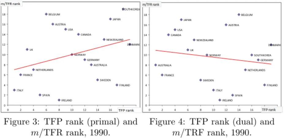
Figure 3 plots 19 economies in the space (TFP rank, m/TFR rank) for 1990, using the primal TFP estimates approach.21 Countries in the bottom-left corner are characterized by higher TFP and later births, relative to other countries. The trend line suggests that there exists a positive relationship between the ranks in terms of TFP and in terms of late motherhood. Highly productive economies, such as France, Italy and the Netherlands, are also characterized by a larger share of late births. On the contrary, less productive economies, such as Japan and South Korea, are also characterized by less late motherhood.
ITALY FRANCE UK NETHERLANDS SPAIN BELGIUM AUSTRIA IRELAND USA NORWAY CANADA GERMANY AUSTRALIA SWEDEN NEWZEALAND JAPAN FINLAND S OUTHKOREA DENMARK 0 2 4 6 8 10 12 14 16 18 20 0 2 4 6 8 10 12 14 16 18 20
Figure 3: TFP rank (primal) and m/TFR rank, 1990. AUSTRALIA FRANCE CANADA USA JAPAN UK NEWZEALAND SWEDEN NORWAY ITALY IRELAND AUSTRIA SPAIN BELGIUM NETHERLANDS SOUTHKOREA GERMANY FINLAND DENMARK 0 2 4 6 8 10 12 14 16 18 20 0 2 4 6 8 10 12 14 16 18 20
Figure 4: TFP rank (dual) and m/TRF rank, 1990.
But while Figure 3 supports a positive relationship between TFP and late fertility, Figure 4, which relies on the dual TFP estimates, does not exhibit an
1 9That dual approach relies on the well-known equivalence, under constant returns to scale, between total output and total factor payments, implying that the growth rate of TFP can be deduced either from the comparison of output growth with input growth (primal approach), or from the growth of factor prices (dual approach), provided one knows the share of each input in the production process.
2 0Note that the 19 countries under study have total fertility rates that are sometimes close to the replacement rate (for instance for the US and New Zealand), but sometimes signi…cantly lower (for instance in Germany and Italy). That di¤erence is somewhat problematic, as the hypothesis we test concern economies with replacement fertility (see below).
increasing pattern. The trend line is here (weakly) decreasing, which does not support the TFP-based explanation of birth timing.
Hence, the observed relationship between TFP and late motherhood does not seem to be robust to the methodology used for productivity measurement. When we take the average TFP ranking on the two approaches to productiv-ity measurement (primal and dual), we obtain a weakly increasing relationship (Figure 5). But this can hardly be regarded as a strong support for a TFP-based explanation of the observed fertility timing. The reason is that many countries, such as Ireland, the Netherlands, Norway and Austria are very close in terms of productivity, but very distant in terms of fertility timing. Hence TFP di¤er-entials cannot be the unique factor driving the timing of births. If one restricts the sample to countries whose TFR is su¢ ciently close to the reproduction rate in 1990 (Figure 6), the positive relationship between TFP and late motherhood becomes slightly steeper, suggesting that intercountry heterogeneity in terms of total fertility may have caused some noise in our comparisons.
FRANCE UK ITALY USA CANADA AUSTRALIA SPAIN NETHERLANDS AUSTRIA IRELAND NORWAY BELGIUM JAPAN SWEDEN NEWZEALAND GERMANY SOUTHKOREA FINLAND DENMARK 0 2 4 6 8 10 12 14 16 18 20 0 2 4 6 8 10 12 14 16 18 20
Figure 5: TFP rank (average) and m/TFR rank, 1990. FRANCE UK NETHERLANDS IRELAND USA NORWAY AUSTRALIA NEWZEALAND 0 1 2 3 4 5 6 7 8 9 0 1 2 3 4 5 6 7 8 9
Figure 6: TFP rank (average) and m/TFR rank, 1990 (subsample).
More generally, those simple cross country comparisons could only inform us on the validity of the TFP-based explanation of birth timing provided all countries are identical in all other aspects, which is hardly the case. In order to avoid the di¢ culties raised by unobserved heterogeneity across countries, the next subsection will focus on a single country, the United States, and try to compare late fertility patterns and TFP patterns.
5.2
TFP and fertility timing in the U.S.
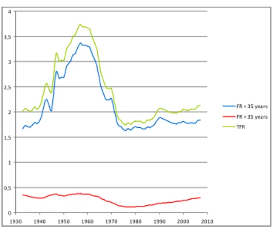
In order to assess the TFP-based hypothesis for the U.S., we will rely on TFP estimates by Fernald (2011), and on age-speci…c fertility rate from the Human Fertility Database. Regarding the period under study, we will focus on the period after 1988, in such a way as to be as close as possible to a period with replacement fertility (TFR close to 2). As shown on Figure 7, the proportion of births beyond age 35 has been growing strongly during that period.
0 0,5 1 1,5 2 2,5 3 3,5 4 1930 1940 1950 1960 1970 1980 1990 2000 2010 FR < 35 years FR > 35 years TFR
Figure 7: Fertility rate before age 35 and after age 35, and total fertility rate,
US, 1933-2007.
If we plot, in a simple diagram, the annual growth rate of the share of late fertility in total fertility, against the annual growth rate of TFP, one obtains an unambiguously increasing relationship, whatever the concept of TFP that is used. That robust increasing relationship appears on Figure 8, which relies on TFP estimates for the whole business sector, and on Figures 9 and 10, which are based on (respectively unadjusted and utilization-adjusted) TFP estimates for consumption goods (i.e. non-equipment goods).
-0,01 -0,005 0 0,005 0,01 0,015 0,02 0,025 0,03 0,035 0,04 0,045 -0,01 0 0,01 0,02 0,03 0,04 Fig. 8: TFP growth (business) and m/TFR growth. -0,01 -0,005 0 0,005 0,01 0,015 0,02 0,025 0,03 0,035 0,04 0,045 -0,02 -0,01 0 0,01 0,02 0,03 Fig. 9: TFP growth (non-eq.) and m/TFR growth. -0,01 -0,005 0 0,005 0,01 0,015 0,02 0,025 0,03 0,035 0,04 0,045 -0,02 -0,01 0 0,01 0,02 0,03 Fig. 10: TFP growth (non-eq., uti-adj.) and
m/TFR growth. Those simple graphs suggest that, over the period 1988-2007, the higher the annual TFP growth was, the larger the postponement of births was. This is exactly in conformity with the TFP-based rationalization outlined from the extended Barro-Becker framework.
In sum, this section does not have the pretension to show that the TFP-based explanation is valid, nor that it is better than a cost-based explanation.22 More
2 2Further empirical assessments will have to be made, while taking into account identi…ca-tion di¢ culties due to unobserved heterogeneity, endogeneity and other potential biases.
modestly, that section suggests that the extended Barro-Becker model is, at …rst glance, not incompatible with the data, since one of its major predications …ts the data. When one reminds that such a qualitative test sometimes su¢ ces to question the relevancy of a model - such as Doepke’s (2005) rejection of the Barro-Becker model for the mortality/fertility relationship - the material provided in this section is at least encouraging for further empirical tests of the extended Barro-Becker model in the context of changing fertility timing.
6
Conclusions
The postponement of births constitutes a major demographic stylized fact of our times. The present paper proposed to extend the canonical fertility model of Barro and Becker (1989), to examine whether standard economic fertility models can help us to rationalize observed fertility timing tendencies.
For that purpose, we introduced an additional reproduction period in the Barro-Becker OLG model. That extension allowed us to examine how individ-uals can, under dynastic altruism, solve the dilemma between early and late children. Whereas the former are consumed earlier, they are also, in general, associated with a longer period of coexistence, which may lead to additional opportunity costs in comparison to later children.
In a …rst stage, we showed that, at the temporary equilibrium, the optimal timing of births is strongly dependent on the cost structure of early and late children, in terms of goods and in terms of time. If late children are more costly than early children during their childhood, and if early children are no longer time-consuming once adult, the optimal fertility pro…le only involves early children. But if early children who become adults are, to some extent, still time-consuming for their parents, then there is some room for late children, especially if medical advances, such as assisted reproductive technologies, have reduced the direct cost of late children.
In a second stage, focusing on a stationary equilibrium with stationary pop-ulation size, we showed that an improvement in TFP tends, in general, to shift steady-state optimal fertility pro…le towards more late births. Hence the ex-tended Barro Becker model proposes not one, but two distinct plausible expla-nations for the postponement of births: either a change in the direct costs of early and late children, or, alternatively, a rise in TFP.
Cross country comparisons in the OECD suggest that the empirical testing of the TFP hypothesis depends signi…cantly on how productivity is measured. Focusing on the U.S., we showed that there exists a positive correlation between TFP annual growth and the annual growth of late fertility, in conformity with what the extended Barro-Becker model suggests. But further empirical investi-gations will have to be done in the future, to be able to assess the plausibility of the cost hypothesis and the TFP hypothesis for changes in fertility timing.
7
References
Ayiar, S. & Dalgaard, C-J. (2005): Total factor productivity revisited: a dual approach to development accounting, IMF Sta¤ Papers, 52 (1), 82-102.
Barro, R. & Becker, G. (1989): Fertility choice in a model of economic growth, Econo-metrica, 57 (2), 481-501.
Cigno, A. & Ermisch, J. (1989): A microeconomic analysis of the timing of births, Euro-pean Economic Review, 33, 737-760.
D’Albis, H., Augeraud-Véron, E. & Schubert, K. (2010): Demographic-economic equilibria when the age at motherhood is endogenous. Journal of Mathematical Economics, 46(6), 1211-1221.
Doepke, M. (2005): Child mortality and fertility decline: does the Barro-Becker model …t the facts?, Journal of Population Economics, 18 (2), 337-366.
Ermisch, J. (1988): The econometric analysis of birth rate dynamics in Britain. The Journal of Human Resources, 23(4), 563-576.
Ermisch, J. & Ogawa, N. (1994): Age at motherhood in Japan. Journal of Population Economics, 7, 393-420.
Fernald, J. (2011): Utilization-adjusted quarterly TFP series for the US business sector. Federal Reserve Bank of San Francisco.
Gustafsson, SS. (2001): Optimal age at motherhood. Theoretical and empirical con-siderations on postponement of maternity in Europe, Journal of Population Economics, 14, 225-247.
Heckman, J. & Walker, J. (1990): The relationship between wages and income and the timing and spacing of births: evidence from Swedish longitudinal data, Econometrica, 58, 1411-1441.
Human Fertility Database. Max Planck Institute for Demographic Research (Germany) and Vienna Institute of Demography (Austria).
Available at www.humanfertility.org (data downloaded on 13/01/2012).
Joshi, H. (2002): Production, reproduction, and education: women, children and work in a British perspective. Population and Development Review, 28, pp. 445-474.
Lee, R. (2003): The demographic transition. Three centuries of fundamental change, Journal of Economic Perspectives, 17 (4), 167-190.
Pestieau, P. & Ponthiere, G. (2011): Optimal fertility along the lifecycle, CORE DP 2011-33.
Schultz, T.P. (1985): Changing world prices, women’s wages and the fertility transition: Sweden 1860-1910, Journal of Political Economy, 93, 1126-1154.
United Nations Population Division/DESA - Fertility and Family Planning Section: World Fertility Data 2008.
Available at http://www.un.org/esa/population/publications/WFD%202008/Main.html
8
Appendix
Bequests timing To illustrate why the mere fact of receiving bequests at the time of the death of parents would introduce di¤erent budget constraints
within a given cohort, depending on the age of parents, let us derive the in-tertemporal budget constraint in the two cases. When the bequest is received at the death of the parent, the budget constraint of a young adult born from a young parent is:
(1 bnt)wt= ct+ st+ ntet
If he receives a bequest kt+1from his parent at his death, his budget constraint at t + 1 is:
wt+1(1 Bmt+1 hnt)+st(1+rt+1)+(1+rt+1)kt+1= dt+1+mt+1Et+1+(nt+mt+1)kt+2 Hence his intertemporal budget constraint is:
wt(1 bnt)+ wt+1(1 Bmt+1 hnt) 1 + rt+1 +kt+1= ct+ntet+ dt+1+ mt+1Et+1+ (nt+ mt+1)kt+2 (1 + rt+1)
For an agent born at the same time, but from an old parent, the two budget constraints are:
wt(1 bnt) + (1 + rt)kt = ct+ st+ ntet
wt+1(1 Bmt+1 hnt) + (1 + rt+1)st = dt+1+ mt+1Et+1+ (nt+ mt+1)kt+2 From which the intertemporal budget constraint is
wt(1 bnt)+ wt+1(1 Bmt+1 hnt) 1 + rt+1 +(1+rt)kt= ct+ntet+ dt+1+ mt+1Et+1+ (nt+ mt+1)kt+2 1 + rt+1
Thus the intertemporal budget constraint di¤ers for agents born at the same point in time, from young or old parents. The overall lifetime spending (RHS) is the same in the two cases, but the lifetime resources (LHS) di¤ers: those born from older parents bene…t from the bequests earlier in their own lifecycle, which makes them richer if one considers an economy at the steady-state (under r > 0). As a consequence, the mere passage of time would lead, under those alterna-tive budget constraints, to an explosion of intracohort heterogeneity, between children from parents, grand-parents etc. of di¤erent ages.
Proof of Lemma 1 In order to compare the derivatives @Nt+1+j
@nt and @Nt+1+j @mt , remember that Nt+1= Ntgt+1= Nt nt+ mtNt 1 Nt . Hence we have: @Nt+1 @nt = Nt @Nt+1 @mt = Nt 1
@Nt+2 @nt = Ntgt+2+ Nt+1 mt+1NtNt N2 t+1 = Nt gt+2 mt+1 gt+1 = Ntnt+1 @Nt+2 @mt = Nt 1gt+2+ Nt+1 mt+1NtNt 1 N2 t+1 = Nt 1 gt+2 mt+1 gt+1 = Nt 1nt+1 @Nt+3 @nt = Ntnt+1gt+3+ Nt+2 mt+2NtNt+2 mt+2Nt+1Ntnt+1 N2 t+2 = Nt[nt+1nt+2+ mt+2] @Nt+3 @mt = Nt 1nt+1gt+3+ mt+2Nt 1 Nt+2 Nt+1nt+1 Nt+2 = Nt 1[nt+1nt+2+ mt+2] :::
or, in general terms:
@Nt+1+j @nt = Nt Nt 1 @Nt+1+j @mt
Thus, whether the marginal impact of raising early fertility is larger than the marginal impact of raising late fertility depends on whether the cohort size is growing over time or not. If Nt > Nt 1 or gt > 1, we necessarily have, everything else being unchanged, that: @Nt+1+j
@nt >
@Nt+1+j
@mt .
Proof of Proposition 2 Note that, in general, we have: @Nt+1+j
@Nt+1 = j+1Y k=1 gt+k, and @N@nt+1+jt = @N@Nt+1+jt+1 @N@nt+1t = Nt j+1Y k=1 gt+k. Hence, imposing gt = g = 1 for all gt leads to @N@Nt+1+jt+1 = 1, and to Nt+j = 1 for all t. Hence, the FOC for optimal early fertility is, at the stationary equilibrium with stationary population: 1 X j=0 t+1+j(1 ") [v(c ) + v(d )] = 1 X j=0 zt+1+j c + d 1 + r + ztbw + zt+1hw + zte + 1 X j=0 zt+1+jn e + 1 X j=0 zt+1+jm E 1 X j=0 zt+1+j(1 bn )w 1 X j=0 zt+2+j(1 Bm hn )w
Substituting for on the basis of the FOC for optimal m , we obtain 1 X j=0 t+1+j(1 ") [v(c ) + v(d )] 1 X j=0 t+1+j(1 ") [v(c ) + v(d )] = 1 X j=0 zt+1+j[c +1+rd ]+ztbw +zt+1hw +zte + 1 X j=0 zt+1+jn e + 1 X j=0 zt+1+jm E 1 X j=0 zt+1+j(1 bn )w 1 X j=0 zt+2+j(1 Bm hn )w 1 X j=0 zt+1+j[c +1+rd ]+ztBw + ztE + 1 X j=0 zt+1+jn e + 1 X j=0 zt+1+jm E 1 X j=0 zt+1+j(1 bn )w 1 X j=0 zt+2+j(1 Bm hn )w
which can be simpli…ed to:
Bw + E = bw + hw 1 + r + e
Proof of Corollary 1 Substituting for wages and interest rate:
w = (1 )A = (1 )A A 1 1 = (1 ) 1 A 1 1 1 1 r = A ( ) 1= A 1 A = 1 in the condition: Bw + E = e + bw + hw 1 + r yields: B(1 ) 1 A 1 1 1 1 + E = e + b(1 ) 1 A 1 1 1 1 + h(1 ) 1 A11 h 1 i1 1 +1 From which the three cases of Proposition 2 can be expressed as:
if (B b h) (1 ) 1 A11 h 1 i1 > e E then n > 0, m = 0 if (B b h) (1 ) 1 A 1 1 h 1 i1 = e E then n > 0, m > 0 if (B b h) (1 ) 1 A11 h 1 i1 < e E then n = 0, m > 0 Assuming that (B b h) < 0 and e E < 0, those conditions can be rewritten as the conditions in Corollary 1.