Anomaly detection methods for unmanned underwater vehicle performance data

Anomaly Detection Methods for Unmanned Underwater Vehicle Performance Data

by

William Ray Harris

B.S., Mathematics US Naval Academy (2013) Submitted to the Sloan School of Management in partial fulfillment of the requirements for the degree of

Master of Science in Operations Research at the

MASSACHUSETTS INSTITUTE OF TECHNOLOGY

MASSACHUSETTS INSTITUTE OF TECHNOLOLGY

JUN 22 2015

LIBRARIES

June 2015

William Ray Harris, MMXV. All rights reserved.

The author hereby grants to MIT and The Charles Stark Draper Laboratory, Inc. permission to reproduce and to distribute publicly paper and electronic copies of

this thesis document in whole or in part.

A uthor ... C ertified by ... C ertified by ... MIT Accepted by ...

Sig

Signature redacted

Sloan School of Management

M<y 15, 2014

Signature redacted

Dr. Vichael J. Ricard Laboratory Technical Staff Charles Stark Draper Laboratory, Inc.

Thesis Supervisor

Signature redacted

Prof. Cynthia Rudin Associate Professor of Statistics CSAIL and Sloan School of Management

(5Tlis Supervisor

nature redacted

Pro . imitris Bertsimas Boeing Professor of Operations Research Co-Director, Operations Research Center

Anomaly Detection Methods for Unmanned Underwater

Vehicle Performance Data

by

William Ray Harris

Submitted to the Sloan School of Management on May 15, 2014, in partial fulfillment of the

requirements for the degree of Master of Science in Operations Research

Abstract

This thesis considers the problem of detecting anomalies in performance data for unmanned underwater vehicles(UUVs). UUVs collect a tremendous amount of data, which operators are required to analyze between missions to determine if vehicle sys-tems are functioning properly. Operators are typically under heavy time constraints when performing this data analysis. The goal of this research is to provide opera-tors with a post-mission data analysis tool that automatically identifies anomalous features of performance data. Such anomalies are of interest because they are often the result of an abnormal condition that may prevent the vehicle from performing its programmed mission. In this thesis, we consider existing one-class classification anomaly detection techniques since labeled training data from the anomalous class is not readily available. Specifically, we focus on two anomaly detection techniques: (1) Kernel Density Estimation (KDE) Anomaly Detection and (2) Local Outlier Factor. Results are presented for selected UUV systems and data features, and initial find-ings provide insight into the effectiveness of these algorithms. Lastly, we explore ways to extend our KDE anomaly detection algorithm for various tasks, such as finding anomalies in discrete data and identifying anomalous trends in time-series data. Thesis Supervisor: Dr. Michael J. Ricard

Title: Laboratory Technical Staff Charles Stark Draper Laboratory, Inc. Thesis Supervisor: Prof. Cynthia Rudin Title: Associate Professor of Statistics

Acknowledgments

There are many to whom I owe thanks for both the completion of this thesis and my experience at MIT. Firstly, I would like to thank Dr. Michael Ricard of Draper Laboratory. His support over the past two years has been invaluable. His genuine concern for my well-being and personal success has made my time at MIT a very rewarding experience.

I would like to thank the Navy, Draper Laboratory, and the Operations Research Center for giving me the opportunity to pursue a Master's degree. Studying oper-ations research at MIT has been an amazing educational opportunity that I believe will forever enrich my life and career.

I am also grateful to Dr. Cynthia Rudin for her guidance and support. She has been a tremendous resource for all of the roadblocks that I encountered throughout the completion of this thesis.

I would also like to thank employees of NUWC and WHOI for taking the time to help me with my research. In particular, I would like to thank Tom Merchant and Nathan Banks, along with others at NUWC for sharing their technical knowledge of the UUVs that I researched for this thesis. I would also like to thank Tom Austin, Mike Purcell, and Roger Stokey of WHOI for providing the data and software used in this research, and also for sharing their technical knowledge of UUVs.

Lastly, I would not have had such a great experience at MIT without the love and support of my family and friends. Classes at MIT were an enjoyable experience with the help of my friends in the ORC. I would also like to thank Rob, Casey, and Amy, my wonderful office mates at Draper Lab, for their friendship and support.

The views expressed in this thesis are those of the author and do not reflect the official policy or position of Charles Stark Draper Laboratory, the United States Navy,

Department of Defense, or the U.S. Government.

Contents

1 Introduction

1.1 Motivation . . . . 1.2 General Problem Statement

1.3 Approach ... 1.4 Contributions . . . . 1.5 Thesis Organization. . . . . 2 UUV Background 2.1 R E M U S . . . . 2.2 M A RV . . . . 3 Anomaly Detection Overview

3.1 B ackground . . . . 3.2 Characteristics of Anomaly Detection Problems . . . . 3.2.1 Types of Anomalies . . . . 3.2.2 Nature of Data . . . .. 3.2.3 Availability of Labeled Data . . . . 3.2.4 O utput . . . . 3.2.5 Characteristics of UUV Anomaly Detection . . . . 4 One-Class Classification Methods

4.1 Statistical Methods . . . . 4.1.1 Parametric Techniques . . . . 15 15 16 17 17 18 19 19 22 25 25 26 27 30 31 33 33 37 37 38 . . . . . . . . ... . . . . . . . .

4.1.2 Non-parametric Techniques . . . . 41

4.2 Distance Based Methods . . . . 43

4.2.1 k-Nearest Neighbors . . . . 44

4.2.2 Local Outlier Factor (LOF) . . . . 45

4.2.3 Clustering . . . . 47

4.3 One-Class SVM . . . . 50

4.4 Discussion . . . . 53

5 Kernel Density Estimation: Parameter Selection & Decision Bound-aries 57 5.1 Parameter Selection . . . . 58

5.2 Computing Decision Boundaries . . . . 61

5.3 Discussion . . . . 64

6 Experimentation 67 6.1 Model Performance . . . . 67

6.2 REMUS Pitch Data Analysis . . . . 69

6.2.1 Model Selection . . . . 72

6.2.2 R esults . . . . 74

6.3 REMUS Thruster Data . . . . 75

6.3.1 Model Selection . . . . 78

6.3.2 R esults . . . . 80

6.4 MARV Thruster Data . . . . 81

6.4.1 Model Selection . . . . 81

6.4.2 R esults . . . . 82

6.5 Discussion . . . . 83

7 Extending KDE Anomaly Detection Technique 85 7.1 Incorporating New Vehicle Data . . . . 86

7.2 Discrete Data . . . . 91

7.4 D iscussion . . . . 95

8 Conclusion 97

8.1 Summary of Results and Contributions . . . . 97 8.2 Future Work . . . . 98

List of Figures

2-1 REMUS 600 - Autonomous Underwater Vehicle[1] . . . . 21 2-2 REMUS 6000 - Autonomous Underwater Vehicle[1] . . . . 21 2-3 MARV - Autonomous Underwater Vehicle[2] . . . . 23 3-1 Illustration of point anomalies in artificially generated bivariate data 28 3-2 Illustration of contextual anomaly in artificially generated periodic data 29 3-3 Illustration of collective anomaly in artificially generated time-series data 30 4-1 Gaussian Model Based Anomaly Detection for Fabricated Data . . . 40 4-2 Kernel Density Estimate for univariate data . . . . 43

4-3 Illustration of data set suitable for Local Outlier Factor Anomaly De-tection . . . . 46 5-1 Kernel Density Estimate using Bowman & Azzalini Heuristic

Band-width for (a) Gaussian and (b) Mixture of Gaussians . . . . 61 5-2 KDE Approximation and Decision Boundary for Univariate Gaussian 64 5-3 Illustration of (a) KDE approximation for Multivariate PDF (b)

Deci-sion Boundary for Multivariate PDF . . . . 64 6-1 Example of (a) Normal Pitch Data and (b) Faulty Pitch Data . . . . 70 6-2 Performance Measures vs. log(a) for REMUS 600 Pitch Test Data

Features .. .. ... . . . .. . . . . .. . . . . ... 73 6-3 Performance Measures on Pitch Test Data vs. ThresholdLOF for

opti-m al k . . . . 74 6-4 F-Measure vs. k for ThresholdLOF 2 . . . . . . .. . . . 75

6-5 Pitch Data Decision Boundaries with (a) Training Data and a = 0.025 (b) Test Data and a = 0.025 (c) Training Data and a = 0.075 (d) Test Data and a = 0.075 . . . . 76 6-6 Example of (a) Normal Thruster Data and (b) Faulty Thruster Data 77 6-7 Performance Measures vs. log(a) for REMUS 600 Pitch Test Data

Features ... _{. . . . 78}

6-8 Performance Measures on Thruster Test Data vs. ThresholdLOF for optim al k. . . . . 79 6-9 Thruster Data Decision Boundaries with (a) Training Data and a =

0.075 (b) Test Data and a = 0.075 . . . . 80 6-10 Performance Measures vs. log(a) for MARV Pitch Test Data Features 82 6-11 MARV Thruster Data Decision Boundaries with (a) Training Data and

a = _{0.05 (b) Test Data and a = 0.05 . . . . 83}

7-1 Illustration of (a) Anomalous Trend in Feature 1 and (b) Bivariate Data Set in Anomalous Trend Example . . . . 88 7-2 Decision Boundaries for Various Training Sets in Anomalous Trend

E xam ple . . . . 89 7-3 Number of Anomalies per Window vs. Sliding Window index for

Anomalous Trend Example . . . . 92 7-4 Histogram of REMUS 6000 Faults with Decision Boundary . . . . 93 7-5 REMUS 6000 Pitch Data Features with Previous REMUS 600 Decision

List of Tables

2.1 REMUS 600 and REMUS 6000 Vehicle Specifications . . . . 20 2.2 MARV Vehicle Specifications . . . . 22 6.1 Decision Classification Table . . . . 68 6.2 KDE & LOF Performance Measures for REMUS Pitch Data Experiment 75 6.3 KDE & LOF Performance Measures for REMUS Pitch Data Experiment 80 6.4 KDE & LOF Performance Measures for MARV Pitch Data Experiment 83

Chapter 1

Introduction

1.1

Motivation

Unmanned underwater vehicles (UUVs) are utilized both commercially and by the military for a variety of mission categories, including oceanography, mine counter-measures (MCM), and intelligence, surveillance and reconnaissance (ISR)

[6].

Many of these mission categories require that UUVs traverse as much area as possible, and, due to resource constraints, in a limited amount of time. As a result, UUV opera-tors will typically seek to minimize the turnaround time between missions in order to maximize the amount of time that a vehicle is in the water and performing its programmed mission.

One constraint when attempting to minimize the turnaround time between sor-ties is the need for operators to perform post-mission data analysis. UUVs collect large amounts of data on every mission. The collected data often contains hundreds of variables from a variety of different sensors, and each variable typically contains thousands of time-series data points. Due to the limitations of underwater commu-nications, operators are often unable to retrieve this data in real time. Thus, data analysis must be performed post-mission, after the vehicle has come to the surface and data has been uploaded.

Post-mission data analysis is performed to ensure that the vehicle is behaving as expected. Operators must check that the vehicle has adequately performed its

programmed mission, and that the vehicle is in good working condition. The task requires an experienced operator who can distinguish between "normal" and "faulty" data. Due to time constraints and the volume of data, this can be a difficult task, even for experienced UUV operators. In addition, it can be difficult to identify anomalous long-term trends in performance data. For example, a certain system may experience degradation over the period of 50 missions. This degradation may be difficult to identify by operators analyzing data from individual missions.

We would like to be able to automate much of the post-mission data analysis task and provide operators with a tool to help identify anomalous features of per-formance data, since anomalous data may be indicative of problem with the vehicle. The desired benefits of such a tool are as follows:

" Improved ability of detecting faults in UUV systems. " Decreased turnaround time between sorties.

" Less operator experience required for post-mission data analysis.

In short, a reliable post-mission analysis tool means less resources (e.g. time, money) being spent per UUV mission, and improved reliability of UUV performance.

1.2

General Problem Statement

This thesis considers the problem of detecting anomalies in UUV performance data.

Anomalies are defined as "patterns in data that do not conform to a well defined

notion of normal behavior"[9]. The assumption in this case is that anomalous data is often indicative of a fault. We define fault, as in

122],

to be "an abnormal condition that can cause an element or an item to fail". By identifying anomalous data, we can

alert UUV operators towards potential faults.

Specifically, we focus on identifying anomalous features of continuous time-series data. Our goal is to build a classifier, trained on historical data, that can distinguish between "normal" and "anomalous" data instances. Our goal is to classify a particular subsystem for a given mission as either anomalous or normal. For this thesis, the

term "normal" will always refer to expected or regular behavior with respect to data instances. We will use the term Gaussian to referring to the probability distribution commonly known as the normal distribution.

1.3

Approach

The problem of anomaly detection is heavily dependent on both the nature of avail-able data and the types of anomalies to be detected

[9].

In this thesis, we explore existing anomaly detection techniques, and we discuss which methods can be effec-tively applied to UUV performance data.

We will take a one-class classification approach to identifying anomalous data fea-tures for a particular UUV subsystem for a given mission. One-class classification anomaly detection techniques assume that all training data is from the same class (e.g. the normal class)[9]. With this approach, we attempt to build a classifier based on normal training data. One issue in this case is that we do not have readily available training data. That is, we do not know whether or not UUV performance data for a given mission contains unmodeled faults. The key assumption that we make is that the majority of UUV missions that we use for training models do not contain faults for the systems of interest.

As will be discussed in Chapter 4, we determine that anomaly detection using kernel density estimation (KDE) is well suited for the problem of UUV anomaly de-tection. Hence, we will primarily focus on the KDE anomaly detection algorithm for our experimentation. The basic approach of this technique is to develop a probability model for the data generating process of features of UUV performance data. We classify future data instances as anomalous if they lie in areas of low probability of our stochastic model.

1.4

Contributions

1. A survey of one class classification methods that are applicable to the problem of UUV anomaly detection.

2. A discussion of parameter selection for our KDE anomaly detection algorithm. 3. Development of an algorithm for computing decision boundaries based on our

KDE models.

4. Experimental results for selected data features for UUV subsystems. We com-pare the KDE anomaly detection algorithm with another one-class classification method called Local Outlier Factor (LOF).

5. A discussion of extending our KDE algorithm for various purposes, namely, (1) detecting anomalies in discrete data, (2) incorporating new data into our KDE models while accounting for potential anomalous trends, and (3) using previous KDE models for new UUVs.

1.5

Thesis Organization

Chapter 2 of this thesis gives an overview of the UUVs and data sets that were used in this research. Chapter 3 provides a description of the anomaly detection problem in its most general form. In this chapter, we discuss the characteristics of the UUV anomaly detection problem, and conclude that one-class classification methods are suitable for this problem. In Chapter 4, we explore existing one-class classification methods that may be suitable for UUV anomaly detection. In chapter 5, we discuss parameter selection for our KDE anomaly detection algorithm, and we also demonstrate how to compute decision boundaries for our classifier. In Chapter 6, we show experimental results for selected UUV subsystems and data features. Lastly, Chapter 7 is a discussion of extending our KDE anomaly detection algorithm for various purposes.

Chapter 2

UUV Background

The UUVs discussed in this thesis are the Remote Environmental Monitoring Unit (REMUS) series of vehicles and the Mid-Sized Autonomous Reconfigurable Vehicle (MARV). In this section, we will discuss the systems and sensor payloads of these vehicles, as well as operational capabilities. We will also describe the data sets that were available for this research.

2.1

REMUS

The REMUS series of vehicles was developed by Woods Hole Oceanographic Institute (WHOI), and is currently manufactured by Hydroid, Inc. The goal of the REMUS project was to develop a UUV that could collect accurate oceanographic measure-ments over a wide area, at a small cost. The first REMUS was built in 1995[15].

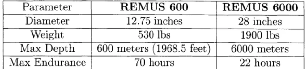
Today, the REMUS series consists of the six types vehicles of varying sizes, spec-ifications, and capabilities. In this research, we had access to data from two types of vehicles, namely the REMUS 600 and the REMUS 6000. The specifications of these two vehicles are given in table 2.1. The most notable difference is that the REMUS 6000 is larger, and capable of operating at depths of up to 6000 meters

[15].

REMUS vehicles maneuver using a propeller and fins. They are powered by rechargeable lithium ion batteries, which must either be recharged or replaced af-ter a mission. There are several ways that a REMUS can obtain a position fix, which

Parameter REMUS 600 REMUS 6000

Diameter 12.75 inches 28 inches

Weight 530 lbs 1900 lbs

Max Depth 600 meters (1968.5 feet) 6000 meters

Max Endurance 70 hours 22 hours

Table 2.1: REMUS 600 and REMUS 6000 Vehicle Specifications

is an estimate of the vehicle's position in the water. The most accurate method is through GPS, but this requires that the vehicle is on the surface since GPS signals will not travel through water. When the vehicle is beneath the surface, it can recieve an acoustic fix by measuring distances from underwater transponders. The position of these transponders is known, and the vehicle can measure distance to and from the transponders by measuring the time that an acoustic ping takes to reach the transponder. Lastly, the vehicle can use dead reckoning using sensor measurements from the Inertial Navigation System (INS) and Acoustic Doppler Current Profiling (ADCP). Dead reckoning is the process of estimating the vehicles position by advanc-ing position from a previous fix based on measurements of velocity and angle through the water.

In addition to the INS and ADCP, the REMUS can be fitted with a variety of sen-sors, depending on mission requirements. Sensors that are commonly utilized include side scan sonar, conductivity & temperature, acoustic imaging, and sub-bottom pro-filing sensors. The ability to customize the REMUS sensor payload allows the vehicle to perform a variety of missions. These missions can be programmed on a laptop computer using the REMUS Vehicle Interface Program (VIP). Typical REMUS ap-plications include[16]:

" Mine Counter Measure Operations " Hydrographic Surveying

" Search & Salvage Operations " Scientific Sampling & Mapping " Debris Field Mapping

Figure 2-1: REMUS 600 - Autonomous Underwater Vehicle[1]

Figure 2-2: REMUS 6000 - Autonomous Underwater Vehicle[1]

REMUS Data Sets

There are two collections of REMUS mission data that were obtained for this research. The first collection is from three separate REMUS 600 vehicles that combined to per-form 282 missions between 2011 and 2014. This mission data was obtained from the Naval Undersea Warfare Center, Division Newport (NUWC-NPT). The second col-lection of mission data is from two REMUS 6000 vehicles. The data covers 72 deep water surveying missions conducted by WHOI operators in 2009.

The data available for each mission is similar for both the REMUS 600 and RE-MUS 6000 collections. Each mission contains over 100 variables, and each variable contains thousands of data points that are in time-series. Of these variables, we are interested in those that a REMUS operator might analyze between missions to iden-tify vehicle faults. According to REMUS operators at WHOI and NUWC-NPT, some variables that are typically analyzed after each mission are thruster output, vehi-cle control data (e.g. pitch, yaw, etc.), and navigation performance data (e.g. frequency of acoustic fixes). Hence, we will focus on identifying anomalous missions based on these variables.

In addition to the time-series data collected on each mission, the REMUS vehicle

maintains a fault log. This log contains a record of events that the REMUS is pro-grammed to identify during a mission. Some of these are normal occurrences, such as the vehicle dropping an ascent weight before driving to the surface. Other events are modeled faults, such as the vehicle not be able to dive below the surface of the water. Again, for this thesis we are interested in identifying previously unmodeled faults, and not those that are identified in the fault log.

2.2

MARV

The Mid-Sized Autonomous Reconfigurable Vehicle (MARV) was designed and manu-factured by the Naval Undersea Warfare Center. The MARV first became operational in 2004. The vehicle has similar systems, capabilities, and sensor payloads as the RE-MUS. One notable advantage of the MARV vehicle is that it has thruster control capabilities that allow the vehicle to hover. This allows the vehicle to remain in one place, which is ideal for object inspection or stand-off reconnaissance. The vehicle specifications for the MARV are given in table 2.2[7]. The vehicle is powered by a rechargeable lithium ion battery.

Parameter MARV

Diameter 12.75 inches Speed 2-5 knots Max Depth 1500 feet Endurance 10-24 hours

Table 2.2: MARV Vehicle Specifications

The MARV, like the REMUS, has a torpedo shape design (shown in figure 2-3). Also, like the REMUS, the MARV can be fitted with a variety of different sen-sors. Common sensor payloads include side-scan sonar, chemical sensors, bathymet-ric sonar, and video cameras. Typical missions performed by the MARV include the following[7]:

" Water Column Chemical Detection and Mapping " Sonar Survey of Water Columns and Ocean Floor

* Object Inspection

e Stand-off Reconnaissance

MARV Data Set

The MARV data used in this research is from a collection of missions run by operators at NUWC-NPT. The collection contains 128 missions from 2013. Like the REMUS data, each mission contains over 100 variables with thousands of data points in time-series. Each mission contains sensor data as well as vehicle health data (e.g. battery status, thruster output, etc.).

Again, we will focus on variables that are typically analyzed for faults by operators between missions. These include variables related to thruster performance, navigation performance, and vehicle control.

Each MARV mission also generates a vehicle log and fault log. The vehicle log contains a record of each action that the vehicle takes on a mission. For example, it lists every change of direction and every acoustic fix that is obtained. The fault log, unlike the REMUS fault log, only lists a select few casualties, and is usually empty unless there is a fault that results in an aborted mission. Due to the fact that the vehicle log contains a much larger amount of information than the REMUS fault log, it is more difficult to pinpoint events that may be the cause of abnormal performance data for the MARV.

Chapter 3

Anomaly Detection Overview

This chapter provides an overview of the anomaly detection problem in its most general form. We discuss characteristics of anomaly detection problems and determine which existing techniques may be relevant to the problem of anomaly detection for UUV performance data.

3.1

Background

Anomaly detection, or outlier detection, is an important and well-researched problem

with many applications. In existing literature, the terms anomaly and outlier are often used interchangeably. Hodge and Austin

[13]

define anomaly as "an observation that appears to deviate markedly from the other members of the sample in which it occurs". For this thesis, we use the definition given by Chandola, et al., in

[9],

"Anomalies are patterns in data that do not conform to a well defined notion of normal behavior". Approaches to anomaly detection are similar, and often identical, to those of novelty detection and noise detection.

Detecting anomalies is an important problem in many fields, since anomalous data instances often represent events of significance. For UUVs, anomalous data is often an indication of a mechanical fault or some other issue with the vehicle that would require action from an operator. Another example would be an anomalous spending patterns on a credit card. If a credit card is being used more frequently or in areas

outside of typical spending areas, it may be an indication of credit card fraud. Other examples of anomaly detection applications include the following[13]:

" Intrusion Detection - Identifying potential security breaches on computer networks.

" Activity Monitoring - Detecting fraud by monitoring relevant data (e.g. cell phone data or trade data).

" Medical Condition Monitoring - Detecting health problems as they occur (e.g. using heart-rate monitor data to detect heart problems).

* Image Analysis -Detecting features of interest in images (e.g. military targets in satellite images).

* Text Data Analysis - Identifying novel topics or events from news articles or other text data.

The unique attributes of each of these applications make the anomaly detection problem difficult to solve in general. Most anomaly detection techniques are catered toward a specific formulation of the problem. This formulation is determined by certain characteristics of our data and the types of anomalies we are interested in detecting. These characteristics are discussed in the following section.

3.2

Characteristics of Anomaly Detection Problems

Anomaly detection problems have been researched since as early as 1887 [101. Since then, a large number of techniques have been introduced, researched, and tested. The necessity for a broad spectrum of techniques is due to unique characteristics of each application of anomaly detection.

In

[9],

Chandola, et al., list four aspects of anomaly detection problems that can affect the applicability of existing techniques. These four characteristics are types of anomalies that are of interest, the nature of input data, the availability of data labels, and the output of detection. In this section, we will address each of

these characteristics separately and discuss the characteristics of anomaly detection for UUV performance data.

3.2.1

Types of Anomalies

The first characteristic of an anomaly detection problem that we will address is the type of anomalies that are of interest. There are three categories of anomalies that we will discuss, namely point anomalies, contextual anomalies, and collective anomalies[9].

Point Anomalies

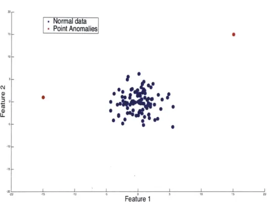
A point anomaly is a single data instance that does not fit to the remainder of the data. This is the simplest type of anomaly, and typically the easiest to detect.

Figure 3-1 shows a two-dimensional data set containing two point anomalies. The normal data is generated from a bivariate Gaussian distribution, and the point anoma-lies were inserted into areas of very low probability.

As an example for UUV data, consider sensor readings for a certain system, say thruster output. If the sensor readings give a single measurement that is outside of normal operational limits, then the measurement would be considered anomalous. Such an anomaly may be due to a problem with thrusters, or due to a sensor that is need of calibration. This is known as limit checking, and is the simplest method of anomaly detection for univariate data.

Contextual Anomalies

A contextual anomaly is a data instance that, given one or more contextual attributes, does not fit to the remainder of the data. Some examples of contextual attributes are time in time series data, position in sequential data, and latitude and longitude in spatial data. Having to account for contextual attributes makes the problem of identifying contextual anomalies more complex than that of point anomalies.

[Normal data-Point Anomalies 10 02 01 101 Feature 1

Figure 3-1: Illustration of point anomalies in artificially generated bivariate data

in April. An inch of snowfall is certainly not anomalous in many parts of the world during the month of April. Additionally, an inch of snowfall in Texas may not be considered anomalous in January. It is the combination of these contextual attributes (location and month) that make such a data instance anomalous. For UUV data, an example of a contextual anomaly would be a 10 degree roll angle while the vehicle is maintaining a straight course. Such a roll angle might be normal if the vehicle is

making a turn, but, given the context, the measurement would be considered

anoma-lous and a possible indication of a fault.

Figure 3-2 illustrates a contextual anomaly. The data used in this plot is fabri-cated, and is meant to represent time-series data with periodic behavior. The anoma-lous data instance, marked in red, would be considered normal without context, since there are a number of similar observations. In order to identify this point as anoma-lous, we must account for the time-series aspect of the data.

T,

LL

I I I I I I

20 40 60 60 600 120 140 160

Time

Figure 3-2: Illustration of contextual anomaly in artificially generated periodic data

Collective Anomalies

Lastly, a collective anomaly is a collection of related data instances that is anoma-lous with respect to the entire data set[9]. The individual data instances may not be considered anomalous on their own. Like contextual anomalies, dealing with col-lective anomalies is typically more complex, since we have to account for additional information (i.e. the relationships between data instances).

An example of a collective anomaly for UUV data would be the absence of a depth reading for a sequence of consecutive depth measurements. It is not uncommon for a vehicle to lose bottom lock, which refers to the event when a vehicle is unable to obtain sensor readings of the ocean floor. If the UUV loses bottom lock, the depth measurement returns 0. Typically, the UUV will regain bottom lock relatively quickly. In this case, we might consider a sequence of twenty consecutive depth readings of 0 as anomalous. Note that for this example it would be easy to transform certain collective anomalies into point anomalies. Instead of measuring depth readings, we

-'Normal" Time-Senes Data

could instead consider the number of observations since the previous non-zero obser-vation. Under this transformation, a sequence of twenty consecutive depth readings of zero would be a point anomaly.

Figure 3-3 illustrates a collective anomaly for fabricated time-series data. The anomalous subset is a sequence that shows very little variance between consecutive observations.

120

I-"Normal" Data_{-Collectve Anomaly}

40

Time

100

Figure 3-3: Illustration of collective anomaly in artificially generated time-series data

3.2.2

Nature of Data

Another characteristic of an anomaly detection problems is the nature of the avail-able data. We refer to each data point as a data instance, and each data instance is made up of one more variables, or attributes. These variables may be continuous, discrete, binary, or categorical. If data instances have one variable, they are said to be univariate. Data instances with two or more variables are multivariate.

We must also consider the relationships between data instances. Two data

in-LL

0

stances, say A and B, are said to be independent if the attributes of A are not affected by the attributes of B, and vice versa. More formally, if A and B are generated by some data generating process, then A and B are independent if

Pr(A U B) = Pr(A) * Pr(B).

That is, the joint probability of data instance A and B both appearing in our data set is equal to the product of the marginal probability of A appearing and the marginal probability of B appearing. Data instances are dependent if

Pr( A U B)

#

Pr(A) * Pr(B).

Time-series and sequential data tend to be highly dependent, since neighboring data instances are typically related.

The applicability of anomaly detection techniques is highly dependent on the nature of our data. Anomaly detection techniques may not be applicable for all types of data. For example, nearest neighbor techniques, which will be discussed in the following chapter, require a distance metric defined over the domain of our data set. Distance metrics (e.g. Euclidean distance) are easy to define over continuous data, but do not translate to categorical data. Furthermore, the majority of existing techniques assume that data instances are independent. Identifying anomalies in dependent data sets typically requires more sophisticated algorithms.

3.2.3

Availability of Labeled Data

Anomaly detection problems are also dependent on the availability of labeled training data. A data instance can be labeled as "anomalous" or "normal". Obtaining labeled training data may be difficult or impractical for a number of reasons. Labeling data may be prohibitively expensive, due to time constraints or the size of a data set. An-other difficulty may be in obtaining data that covers the range of possible anomalies, particularly if anomalous data instances correspond to rare events. Depending on the

availability of labeled data, there are three approaches to anomaly detection, namely supervised, semi-supervised, and unsupervised anomaly detection.

Supervised Anomaly Detection

Supervised anomaly detection methods require labeled training data from both the

"normal" and "anomalous" classes. The goal of supervised anomaly detection is to build a classifier that can distinguish between these two classes. This is also known as two-class classification, and is often done by building probability models for each class. With this strategy, future instances are classified by comparing the conditional probabilities that the instance belongs to each class. Another strategy is to fit classifiers directly, without building probabilistic models. The support vector machine is one such classifier, and does not require any assumptions about the data generating process [171.

Utilizing supervised anomaly detection methods can be difficult. As previously stated, obtaining sufficient labeled training data is often infeasible. Even with training data from both classes there is often the issue of data imbalance. This occurs when the training set contains many more instances from the "normal" class, and is often the case for anomaly detection problems[11].

Semi-Supervised Anomaly Detection

Semi-Supervised anomaly detection methods require data from the "normal" class.

These methods are more widely applicable than supervised methods, since normal data is often readily available for most applications. A common approach for semi-supervised methods is to develop a probabilistic model for normal behavior, and classify future instances as anomalous if they lie in regions of low probability.

Unsupervised Anomaly Detection

Lastly, Unsupervised anomaly detection methods can be used when labeled training data is unavailable. The key assumption for unsupervised methods is that anomalous

data instances appear much less frequently than normal data instances in our training set. As stated in

[9],

if this assumption does not hold true, then these methods can lead to a very high false-alarm rate. These methods are widely applicable, since they do not require labeled data.

3.2.4 Output

The last characteristic of an anomaly detection problem is the desired output to be reported. Chandola, et. al, list two possible outputs: anomaly scores and labels[9].

An anomaly score is a numeric value assigned to a data instance that represents the degree to which the instance is considered anomalous. Typically, higher scores are used for anomalous data instances. An example would be if we create a probabilistic model for normal data under a semi-supervised technique. Suppose we estimate a probability density function, x, for normal data. A reasonable anomaly score for a test point would be the inverse of the density function evaluated at that point. That is, for a point, x, in our test data set, we have

1

score(x) = ^ .

An analyst might sort test data by anomaly score, and then select the instances with the highest scores to analyze further.

The alternative is to output a label, either "anomalous" or "normal". This is typically done by selecting a certain threshold for what is considered anomalous. For many techniques, outputting a label is equivalent to setting a predetermined threshold on anomaly scores. For other techniques, such as SVM, the relationship between an anomaly score and a label is not as straightforward.

3.2.5 Characteristics of UUV Anomaly Detection

We now discuss the characteristics of the UUV anomaly detection problem that is of interest in this thesis. These characteristics will allow us to narrow down potential anomaly detection techniques that may be applicable to our data.

As stated in our problem statement in Chapter 1, the goal of this research is to help operators identify faults in UUV systems that are previously unmodeled. Specifically, we are interested in determining if systems are behaving normally over an entire mission. As discussed in Chapter 2, most UUV performance data is time-series, but we will not address the problem of finding anomalous sequences within this time-series data. According to experienced operators, a vehicle will not typically experience an unmodeled fault and then correct itself in the middle of the mission. For example, if a part of the thruster system breaks, it will remain broken for the entire mission. Instead, we will use features of performance data to identify anomalous system behavior over the course of an entire mission. We must select appropriate features that are indicative of system performance

Our problem is thus to find point anomalies, where our data are specific features of performance data. Each point in our data set corresponds to a feature of time-series data from an individual mission. As an example, suppose we are interested in identifying anomalous thruster behavior. UUVs typically collect time series data of thruster ouput and thruster goal over the course of a mission. A feature that we could use is the average of the difference between thruster output and thruster goal. If thruster data is collected from time t = 1 to T then the feature, Xi, of mission i is:

T

E T hruster Out put (t ) - T hruster Goal (t )

For this problem, we do not have available labeled data. The UUVs of interest do generate a fault log, which is typically an ad hoc list of faults that are previously modeled. The vehicle is programmed to automatically identify these faults, and an operator will be alerted to them by reading through the fault log after a mission. Since we are interested in identifying unmodeled faults, we do not have the luxury of using these fault logs to obtain labeled data. Furthermore, it would be implausible to obtain sufficient labeled data for the following reasons:

* Unmodeled faults are rare relative to modeled faults and normal performance data.

* Unmodeled faults are not well documented.

" Due to the complexity of UUV systems, there is a wide range of possible faults, which may correspond to a wide range of anomalous data.

Due to the lack of labeled data, we will focus on unsupervised anomaly detection methods. Due to the fact that operators are under a time-constraint when perform-ing post-mission data analysis, we will focus on methods that output a label, rather than an anomaly score. This will save operators the step of analyzing a sorted list of anomaly scores.

In conclusion, our goal is to identify anomalous performance data by using fea-tures of time-series data from individual missions. We are interested in methods that output an anomaly label. Due to lack of available labeled data, we will use unsuper-vised methods, and make the assumption that anomalies in our test set are rare. In the following chapter, we will discuss one-class classification methods that could be appropriate for this task.

Chapter 4

One-Class Classification Methods

Based on the characteristics of the UUV anomaly detection problem, we have deter-mined that one-class classification methods are most suitable for identifying anoma-lous features of UUV data. In this chapter, we discuss specific one-class classification methods that may be applicable, namely statistical methods, distance-based meth-ods, and the one-class support vector machine.

These methods can be utilized for both semi-supervised and unsupervised anomaly detection. In the semi-supervised case, we have labeled training data from the normal class. In the unsupervised case, we have unlabeled data, but we rely on the assump-tion that anomalous data instances are rare in our test set. As previously stated, for this research we are assuming that unmodeled faults, which typically correspond

anomalous mission performance data, are rare events.

4.1

Statistical Methods

The general strategy with statistical anomaly detection techniques is to estimate some probability distribution using historical data. The estimated distribution is then used to make a decision on future data points. The key assumption for these techniques, as stated in

[9],

is that "normal data instances occur in high probability regions of a stochastic model, while anomalies occur in the low probability regions of the stochastic model". These methods also rely on the assumption that normal data

instances are independent and identically distributed.

In this section, we will discuss both parametric and non-parametric techniques. The key distinction is that parametric techniques require extra assumptions about our data, namely that the data is generated from a family of probability distributions, and that these distributions have a fixed number of parameters. If these assumptions are correct, then parametric techniques will typically lead to better results. Non-parametric techniques make no assumptions on the underlying distribution of our data.

4.1.1

Parametric Techniques

With parametric techniques we make an assumption about the family of distributions to which the data generating process of interest belongs. Our goal is to estimate a probability density function, fX (x; E), where x is a data instance and

e

represents the parameters of the density function. In other words, we attempt to estimate a probability density function over x, parameterized by . We estimate 6 in one of two ways.

First, we can estimate E by using the maximum likelihood estimate (MLE). This is a function of our training data. The idea of MLE is to find the parameters that max-imize the likelihood that our data was generated by fx(x; 0). Suppose our training data consists of the instances xi E D. The maximum likelihood estimate, E(D)MLE

is given by:

E(D)MLE arg max 17 fx(xi 0).

E xicD

Alternatively, we can incorporate some prior knowledge about our data to find the

maximum a posteriori probability (MAP) estimate for 0. Suppose we have a prior

distribution on our parameters, say g(0). This prior distribution would typically be developed from expert knowledge on the system of interest. From Bayes' theorem, the maximum a posteriori probability estimate, OMAP is given by:

OMAP(D) = arg max _e 11 f(x))

xED P() = argmax

]1

f(xjjE))g(E)

e xiED

Using our estimated parameters,

E,

we can output an anomaly score for a test instance, xi, corresponding to the inverse of the density function evaluated at xi. We can label data instances as anomalous by setting a threshold on the anomaly score. Typically, this threshold is determined by estimating of the frequency of anomalies in our data. As an example, we consider Gaussian model based anomaly detection.

The advantage of MAP estimation is that it allows us to incorporate expert knowl-edge into our probability models. If we have an appropriate prior for

E,

then MAP estimation will likely lead to better results.

Gaussian Model

In this simple example, suppose we have n univariate data instances,

{xi,

X2, ... ,

}=

Dtraining. The assumption in Gaussian model based anomaly detection is that our

data is generated by a univariate Gaussian probability density function with param-eters

E

= {p, a-}. For this example, we estimate our parameters,

e

=

[A,

&], using maximum likelihood estimates. These estimates are given by:

$= [A,]=arg max H fx (xi; [Yo). (4.1)

[IptO xjED

As shown in [18], the values

f

and & that maximize equation 4.1 the sample mean and sample standard deviation, respectively. That is,

n Xi n n (fi - A)2 i=1 n 0.2 0018 0.16 C u . 0.04 -2 0

ata points in test set

stimated PDF

ecision Boundary

-i

-Feature 1 (X) 10 12

Figure 4-1: Gaussian Model Based Anomaly Detection for Fabricated Data Figure 4-1 shows an example for fabricated test data generated from a Gaussian distribution with y = 4, and - = 2. We used maximum likelihood estimates to compute A and & from our test data. For this example, we estimated that 10% of our features are anomalous due to unmodeled faults. We thus compute a 90% confidence interval for data points generated by our estimated PDF. Boundaries for our confidence interval are given by Aftz*&, where z is the point where the cumulative

density function is equal to 010 = 0.05, that is F6(z) = 0.05. Once we have our decision boundary, a test point Xtest is classified as anomalous if it lies outside of our

"'

-- 0

-E -D(

computed confidence interval.

4.1.2

Non-parametric Techniques

With non-parametric techniques, we are not required to make an assumption about the underlying distribution of our data. Similar to parametric techniques, we attempt to estimate the distribution of the data generating process, and we classify test in-stances as anomalous if they fall into regions of low probability. Two non-parametric techniques that were explored in this research are histogram-based anomaly detection,

and anomaly detection using kernel density estimation.

Histogram-Based

Histogram-based anomaly detection is the simplest non-parametric technique avail-able. For univariate data, this involves creating a histogram based on training data, and classifying test instances as anomalous if they fall into bins with zero or few train-ing instances. The key parameter in this case is the size of bins in our histogram. If our bin size is too small, we are more likely to have normal instances fall into bins with few or no training instances. This will lead to a high false alarm rate. On the other hand, if the bin size is too large, we are more likely to have anomalous instances fall into bins with a higher frequency of training data, leading to a higher rate of true negatives[91.

One way to choose a bin size for histogram-based methods would be to estimate the number of unmodeled faults in our training set. We could fix the threshold, start with a large bin size, and decrease bin size until the number of anomalies classified in our training set is approximately equal to our estimate of the number of unmodeled faults. Alternatively, we could fix bin size and adjust our threshold until we achieve the same number of faults in our training set.

Kernel Density Estimation

Kernel density estimation, also known as Parzen Windows Estimation, is a non-parametric technique for estimating a data generating process. A kernel, K(-) is any non-negative function that has mean zero and integrates to one. Two commonly used kernels are the Gaussian kernel (KG) and the Epanechnikov kernel (KE). These kernels are defined by the following equations:

1 -X) KG () = exp(2 V2T 2 3 KE(X) -- 2 4

Given a set of training data, {Xi, ... , X}= Dtraining, and kernel, K(x), we estimate

the probability density function over x with the following equation:

n * h =1 h

where h is a smoothing parameter known as the bandwidth. We can also include h in our characterization of our kernel function, by letting Kh(x) = -K(x/h). If we use Kh, also known as a scaled kernel, our density estimate reduces to the following:

fx(x) = Kh(X - Xi)

n i=1

In words, if we have n training data instances, our density estimate is the average of

n scaled kernel functions, one centered at each of the points in our training set[19j.

Figure 4-2 illustrates a KDE approximation for a univariate PDF. The estimated PDF (black) is the sum of scaled kernel functions (blue) centered at our data (red).

Once we have an estimate for a probability density function, the problem of clas-sifying anomalies is identical to that of parametric statistical methods. We classify a test instance, xest, as anomalous if it lies in an area of low probability. In the following chapter, we will explore methods for computing decision boundaries based

0.25 0.2 015 01 o.osI--KDE PDF Approximation Data

-Scaled Kernel Functions

x

Figure 4-2: Kernel Density Estimate for univariate data

on PDFs estimated using kernel density estimation. We will also explore parameter selection for bandwidth, h.

4.2

Distance Based Methods

Nearest neighbor and clustering algorithms are common in machine learning litera-ture. In this section we will discuss how nearest neighbors and clustering algorithms have been adapted for the purpose of one-class classification. Unlike statistical meth-ods, these techniques do not involve stochastic modeling.

These techniques require a distance metric to be defined between two data in-stances. The distance metric used in this research is Euclidean distance, de. For instances xi, xj E D C R', Euclidean distance is defined as

0

d,(xi,

xj)

= (z - XI)2 + (X2 - X2) +_. . . (X

-_)

- _{(X X-j) - ( i - X).}

Another commonly used distance metric is Mahalanobis, or statistical distance, which takes into account correlation between variables. This is a useful distance metric if we believe that our variables are highly correlated.118].

4.2.1

k-Nearest Neighbors

As stated in

[9],

k-nearest neighbor anomaly detection relies on the assumption that "Normal data instances occur in dense neighborhoods, while anomalies occur far from their closest neighbors". Incorporating k-nearest neighbors for one-class anomaly detection requires the following steps[22]:

1. Store all data instances from training set, Dtraining.

2. Select parameter k and distance metric, d(xi, xj).

3. For each x E Dtraining, identify the k-nearest neighbors in Dtraining. We will

denote the set of k-nearest neighbors of xi as N(xi).

4. Compute an anomaly score for each instance x E Dtraining. The anomaly score

for instance xi is given by the averaged distance from xi to its k-nearest neigh-bors:

anomaly score(xi) = d(xi, xj)

xjEN(xi)

5. Set a threshold, denoted thresholdkia, on anomaly scores. This is determined by our belief of the frequency of faults in our test set. If we believe that a fraction, p, of n missions in our test set contain unmodeled faults, then we

confirmed that our test set contains no unmodeled faults then we would select

thresholdkNN = max {anomaly score(xi) : xi E Dtest}.

6. For a test instance, Xtest e Dtest, identify the k-nearest neighbors within the

training set.

7. Compute the anomaly score for Xtest as in step 4:

anomaly score(xtest) = 1 d(Xtest, xj).

xjEN(xtest)

8. If anomaly score(xtest) > thresholdkNN, classify instance as anomalous. Oth-erwise, classify as normal.

4.2.2

Local Outlier Factor (LOF)

One shortcoming of many distance based techniques, including k-nearest neighbors, is that they only account for global density of our data set. For more complex real-world data sets, our data may contain regions of higher variance. In this case, we would also like to take into account local density when identifying point anomalies.

Consider figure 4-3, which contains two clusters of normal data, as well as a point anomaly. The two clusters contain the same amount of data instances, but the bottom left cluster has a much higher local density. The point anomaly would typically not be identified by conventional k-nearest neighbors or clustering techniques, since it is still closer to its nearest neighbors than instances in the top right cluster.

In 1999, Breunig et. al, developed a distance based anomaly detection technique, similar to k-nearest neighbors, that takes into account local density[5]. This technique is known as local outlier factor (LOF) anomaly detection. Implementing LOF for one-class anomaly detection requires the following steps:

1. Store all data instances from training set, Dtraining. 2. Select parameter, k, and distance metric, d(xi, xj).

* Normal Data - Point Anomaly a 0 0 0 * 0 0 0 * 0 0 0 0 0 0 0 01000 'be 00 0 0 -2 1 1 1 1 1 F1at3 4 1 Feature 1 8b 6 9 10

Figure 4-3: Illustration of data set suitable for Local Outlier Factor Anomaly Detec-tion

3. For each x E Dtraining, identify the k-nearest neighbors in _Dtraining. We will denote the set of k-nearest neighbors of xi as N(xi).

4. For each xi E Dtraining, compute the local density of xi, which is given by:

Local Densityz(xi) =

radius of smallest hypersphere centered at xi containing N(xi) k

max {d(xi, xj)Ixj C N(xi)}

5. For each xi E Dtraining, compute the local outlier factor of xi. This value will serve as an anomaly score, and is given by:

LL

10 ,

LOF(i)' average local density of k-nearest neighbors of xi

local density(xi)

local density(xj)

xjEN(xi)

local density(xi)

6. Set a threshold, denoted thresholdLOF, on anomaly scores. Again, this is de-termined by our belief of the frequency of faults in our test set. If we believe that a fraction, p, of n missions in our test set contain unmodeled faults, then

we select thresholdLOF to be the (p * n)th highest local outlier factor.

7. For a test instance, xtest E Dtest, compute LOF(xtest), using Dtraining to identify

the k-nearest neighbors of xtest.

8. If LOF(xtet) > thresholdLOF, classify instance as anomalous. Otherwise, clas-sify as normal.

4.2.3

Clustering

Clustering is the process of partitioning a data set so that similar objects are grouped together. There is extensive literature available for a number of different clustering techniques. Some common approaches to clustering include[18]:

" Model Based Clustering " Affinity Propagation " Spectral Clustering " Hierarchical Clustering " Divisive Clustering

We will not go into detail about various clustering algorithms in this thesis. In-stead, we will discuss techniques for anomaly detection for data that have already

been clustered. In particular, we assume that our training data set, Dtraining, has

been partitioned into clusters, and our goal is to classify a test instance, Xtest.

Chandola, et al. distinguish between three different categories of cluster-based anomaly detection. These distinctions are based on assumptions about anomalous data instances. The assumptions of the three categories are as follows[9]

" Category 1: Normal data instances belong to clusters, whereas anomalies do not belong to clusters, based on a given clustering algorithm that does not require all data instances to belong to a cluster.

" Category 2: Normal data instances lie close to the nearest cluster centroid, whereas anomalous data instances do not.

" Category 3: Normal data instances belong to large, dense clusters, while anomalies belong to small and sparse clusters.

The first category requires a clustering algorithms that does not force all data in-stances to belong to a cluster. The main idea is to use such a clustering algorithm on the training data set together with the test data point (i.e. use clustering algorithm on Dtraining U Xtest). If xt,,t does not belong to a cluster (or is the only point in a clus-ter), then classify as anomalous. Otherwise, Xtest is classified as normal. An example

of such an algorithm would be hierarchical agglomerative clustering. This technique begins with all data instances as individual clusters, then merges data points one at a time based on a certain distance metric[18]. This category is not well-suited for our problem, since it requires that training data is clustered along with test data. We would prefer a technique in which clustering is done prior to having access to Xtest, in order to save on computation time.

The second category of cluster based anomaly detection requires all data to belong to a cluster. The typical approach would be to partition Dtraining into clusters, and then classify xtest as anomalous if it outside a certain threshold distance from the closest cluster centroid. This is a promising approach if we believe that our perfor-mance data features form distinct clusters.