arXiv:1005.5254v1 [hep-ex] 28 May 2010
Performance of the ATLAS Detector using First
Collision Data
The ATLAS Collaboration
September 12, 2018
Abstract
More than half a million minimum-bias events of LHC collision data were collected by the ATLAS experiment in December 2009 at centre-of-mass energies of 0.9 TeV and 2.36 TeV. This paper reports on studies of the initial performance of the ATLAS detector from these data. Comparisons between data and Monte Carlo predictions are shown for distributions of several track- and calorimeter-based quantities. The good performance of the ATLAS detector in these first data gives confidence for successful running at higher energies.
1
Introduction
In December 2009, the ATLAS detector [1] recorded data from a first series of LHC runs at centre-of-mass energies of 0.9 TeV and 2.36 TeV. When the beams were colliding and declared to be stable by the LHC operators, all main detector components were fully operational and all levels of the trigger and data acquisition system performed as expected, assuring smooth and well mon-itored data taking. The data sample at 0.9 TeV contains nearly 400 000 events recorded with high-quality calorimeter and tracking information, corresponding to an integrated luminosity of approximately 9 µb−1[2]. The data at 2.36 TeV,
36 000 events, which are only used here for calorimeter studies, correspond to approximately 0.7 µb−1. These data sets do not contain very many high-p
T
objects, and therefore do not correspond to the environment for which ATLAS was designed.
The ATLAS detector was thoroughly commissioned and initial calibration and performance studies were done using cosmic ray data recorded during 2008 and 2009. Performance close to design goals was obtained for the different detector components, details can be found in Refs. [3, 4, 5, 6].
This paper presents performance established with data taken in first colli-sions in 2009. The detector components are outlined in Section 2. The trigger and data acquisition performance together with the initial event selection are discussed in Section 3; the simulation to which the data are compared is ex-plained in Section 4. The performance of the inner tracking system is reviewed in Section 5, and the combined analysis of calorimeter data and tracking infor-mation to study electrons and photons is discussed in Section 6. Studies of jets and missing transverse energy, Emiss
in Sections 7 and 8. Finally, kinematic distributions of the first reconstructed muon candidates are shown in Section 9.
2
The ATLAS Detector
The ATLAS detector [1] covers almost the entire solid angle around the nominal interaction point and comprises the following sub-components:
• An inner tracking system: operating inside an axial magnetic field of 2 T, it is based on three types of tracking devices. These are an outer tracker using straw tubes with particle identification capabilities based on transition radiation (Transition Radiation Tracker, TRT), a silicon strip detector (SemiConductor Tracker, SCT) and an innermost silicon pixel detector (Pixel).
• A hybrid calorimeter system: for the electromagnetic portion (EM), the hadronic end-cap (HEC) and the forward calorimeter (FCal) a liquid ar-gon (LAr) technology with different types of absorber materials is used. The central hadronic calorimeter (Tile) is a sampling calorimeter with steel as the absorber material and scintillator as the active medium. The electromagnetic sections use an accordion geometry to ensure fast and uniform response. A presampler detector, to correct for energy losses in the upstream material, is installed in front of the EM calorimeter in the range |η| < 1.8.1
• A large muon spectrometer: an air-core toroid system generates an average field of 0.5 T (1 T), in the barrel (end-cap) region of this spectrometer, resulting in a bending power between 2.0 and 7.5 Tm. Over most of the η-range, tracks are measured by Monitored Drift Tubes (MDT); in the high η-regime the closest of four wheels to the interaction region is instrumented with Cathode Strip Chambers (CSC). Trigger information is provided by Thin Gap Chambers (TGC) in the end-cap and Resistive Plate Chambers (RPC) in the barrel.
• Specialized detectors in the forward region: two dedicated forward de-tectors, the LUCID Cherenkov counter and the Zero Degree Calorime-ter (ZDC). In addition the BPTX, an electrostatic beam-pickup which monitors the timing of the beam near ATLAS and two scintillator wheels (MBTS) were mounted in front of the electromagnetic end-caps to provide trigger signals with minimum bias.
3
Data-Taking Performance and Event Selection
The ATLAS operating procedure in 2009 maintained the calorimeters and TRT in standard operating conditions, but the silicon trackers and muon chambers 1The origin of the coordinate system used to describe the ATLAS detector is the nominal interaction point. The positive x axis is defined as pointing from the interaction point to the centre of the LHC ring, the positive y axis is defined as pointing upwards and the beam direction defines the z axis of a right-handed coordinate system. Transverse momenta are
Table 1: Luminosity-weighted fraction of the time during stable beam operation for which the different detectors were able to take data under nominal conditions.
Pixel SCT TRT LAr Tile MDT RPC TGC
Efficiency [%] 80.9 86.2 100 99.0 100 87.4 88.6 84.4
were at a reduced or ‘standby’ voltage until after stable beams were declared by the LHC. Most of the studies in this paper required the tracking detectors to be in operating conditions and used approximately 400 000 events while the Emiss
T
studies only required the calorimeters and used some 600 000 and 36 000 events at 0.9 TeV and 2.36 TeV respectively. The luminosity-weighted availability of the various sub-detectors (see Section 3.3) during stable beam operations is summarized in Table 1.
3.1
Trigger/DAQ System
The ATLAS trigger and data acquisition (TDAQ) is a multi-level system with buffering at all levels [1]. Trigger decisions are based on calculations done at three consecutive trigger levels. While decisions at the first two levels are pend-ing, the data acquisition system buffers the event data from each sub-detector. Complete events are built after the second level decision. The first level trigger (L1) is largely based on custom built electronics. It incorporates timing from the BPTX and coarse detector information from the muon trigger chambers and the trigger towers of the calorimeters, along with multiplicity information from the MBTS scintillators and the ATLAS forward detectors, LUCID and ZDC. The L1 system is designed to select events at a rate not exceeding 75 kHz from an input rate of 40 MHz and identify regions-of-interest (RoIs), needed by the high-level trigger system (HLT), for potentially interesting physics objects. HLT runs on a processor farm and comprises the second level (L2) and the third level trigger or Event Filter (EF). The L2 system evaluates event characteris-tics by examining the RoIs using more detector information and more complete algorithms. The EF analyzes the L2 selected events again looking at the RoIs’ measurements. The analysis of the complete event is also possible. The output rate is reduced to approximately 200 Hz.
All trigger decisions used were made by the L1 systems as the luminosity was low. Minimum-bias events were triggered by a coincidence between the the BPTX and signals indicating hits in one or both of the MBTS scintillator wheels. However, the functionality of the main L2 and EF algorithms, for example those used for inner track reconstruction and jet finding, were validated by running in ‘passthrough’ mode, i.e. calculating relevant L2 and EF decisions without rejecting events. Important distributions like the vertex position (Fig. 1(a)) were monitored online and different data streams for fast analysis feedback based on L1 trigger decisions were provided. For the December 2009 running period the data-taking efficiency of the overall Trigger/DAQ system, as illustrated in Fig. 1(b), averaged to 90%.
Vertex z [mm] -200 -150 -100 -50 0 50 100 150 200 Entries / 2 mm 0 100 200 300 400 500 ATLAS Data 2009 = 0.9 TeV s (a)
Figure 1: (a) Reconstructed z-vertex distribution calculated online by the higher level trigger for monitoring purposes. The width includes a small contribution from the experimental resolution. (b) Data-taking efficiency for periods with two circulating beams in December 2009.
[ns] MBTS t ∆ -80 -60 -40 -20 0 20 40 60 80 Entries / ns 1 10 2 10 3 10 4 10 5 10 Collisions SingleBeam = 0.9 TeV s ATLAS (a) [ns] MBTS t ∆ -80 -60 -40 -20 0 20 40 60 80 Entries / ns 1 10 2 10 3 10 4 10 5 10 Collisions = 0.9 TeV s ATLAS (b)
Figure 2: Time difference ∆tMBT Sof hits recorded by the two MBTS scintillator
wheels mounted in front of the electromagnetic end-cap wheels on both sides of the ATLAS detector; (a) time difference without any selection and (b) requiring a well-reconstructed vertex.
3.2
Event Selection
To select collision candidates and remove beam-related background two different strategies were employed:
• For those studies based mainly on track information, the presence of a primary vertex, reconstructed using at least three tracks with sufficient transverse momenta, typically pT > 150 MeV, and a transverse distance
of closest approach compatible with the nominal interaction point are required. This selection strategy, which was used in Ref. [2], uses events triggered by a single hit in one of the two MBTS scintillator wheels. • Alternatively, the selection is based on the timing difference of signals
de-tected on both sides of the ATLAS detector. Coincident signals, within a time window of 5 or 10 ns from either the electromagnetic calorime-ters (end-cap or FCal) or from the two MBTS wheels, respectively, are required. The event must again be triggered by an MBTS signal. In case no timing coincidence is found, a two hit MBTS trigger with at least one hit per side is required.
The detailed track quality criteria used for the first strategy vary slightly for the different studies presented and are described later when appropriate.
Without any event selection the MBTS-triggered events contain backgrounds from beam-related events as shown in Fig. 2(a), where the time difference, ∆tMBTS, of MBTS signals recorded on both sides of the ATLAS detector is
de-picted. For events coming from the interaction point ∆tMBTS is small.
Beam-related background produced upstream or downstream should have ∆tMBTS
around 25 ns, with the sign giving the direction. Eighty percent of single beam events are missing timing information on one or both sides and are therefore not shown. Requiring a well-reconstructed vertex with track quality requirements reduces the beam-related background by more than three orders of magnitude while retaining genuine collision events (Fig. 2(b)). There are twelve single-beam events which meet this vertex requirement, but all of them are missing timing information and are not shown.
3.3
Luminosity Measurement
The luminosity during the 2009 ATLAS data-taking period was estimated offline based upon the timing distributions measured by the MBTS. Events with signals detected on opposite ends of the ATLAS detector in the MBTS are counted. After background subtraction the luminosity is calculated using the number of events with a timing difference consistent with particles originating from the interaction point (see Fig. 2), the expected minimum-bias cross section and the event selection efficiency determined from data and Monte Carlo. The MBTS detector is used for the absolute luminosity determination because of its high trigger efficiency for non-diffractive events [2]. The uncertainty on the luminosity, dominated by the understanding of the modelling of inelastic pp interactions, is estimated to be around 20%.
Figure 3 shows the luminosity as a function of time, as measured using the MBTS system as well as with three other techniques: timing in the LAr, the LUCID relative luminosity monitor and particle vertices reconstructed online.
UTC Time: December 12, 2009 14:00 15:00 16:00 17:00 18:00 19:00 ] −1 s −2 [ cm 25 Luminosity/10 0 5 10 15 20 25 30 35 −1 b µ 0.6 (stat+syst) ± dt = 3.0 MBTS L
∫
ATLAS = 0.9 TeV s LAr LUCID norm. to MBTSHLT vertex counting norm. to MBTS MBTS
Data 2009
Figure 3: Instantaneous luminosity measured by the MBTS and LAr, with superimposed the LUCID and HLT vertex counting estimates normalized in such a way to give the same integrated luminosity as measured with the MBTS system. All measurements are corrected for TDAQ dead-time, except LUCID which is free from dead time effects. The short luminosity drop at 14:15 is due to inhibiting the trigger for ramping up the silicon detectors after declaration of stable LHC beams.
The LAr technique has a slightly larger systematic uncertainty in the accepted cross section than that from the MBTS and produces a result which agrees to 4%. The other methods are normalized to the MBTS measurement.
4
Monte Carlo Simulation
Monte Carlo samples produced with the PYTHIA 6.4.21 [7] event generator are used for comparison with the data. ATLAS selected an optimized parameter set [8], using the pT-ordered parton shower, tuned to describe the underlying
event and minimum bias data from Tevatron measurements at 0.63 TeV and 1.8 TeV. The parton content of the proton is parameterized by the MRST LO* parton distribution functions [9].
Various samples of Monte Carlo events were generated for single-diffractive, double-diffractive and non-diffractive processes in pp collisions. The differ-ent contributions in the generated samples were mixed according to the cross-sections calculated by the generator. There was no contribution from cosmic ray events in this simulation. All the events were processed through the ATLAS detector simulation program [10], which is based on GEANT4 [11]. This sim-ulation software has also been systematically compared to test-beam data over the past decade (see e.g. Ref. [12]) and it was constantly improved to describe these data. After the detector simulation the events were reconstructed and analyzed by the same software chain also used for data.
butions, particularly for detectors close to the interaction region. The length of the luminous region, as seen in Fig. 1(a), is approximately half that expected, and the simulated events were re-weighted to match this. The transverse offset in the simulation of about 2 mm cannot be corrected for by this method.
The distributions presented in this paper always show the simulated sample normalized to the number of data events in the figure.
5
Tracking Performance
The inner tracking system measures charged particle tracks at all φ and with pseudorapidity |η| < 2.5. The pixel detector is closest to the beam, covering radial distances of 50 – 150 mm with three layers both in the barrel region and in each end-cap. The innermost Pixel layer (known as the B-layer) is located just outside the beam pipe at a radius of 50 mm. The pixels are followed, at radii between 299 – 560 mm, by the silicon strip detector known as the SCT. This provides 4 (barrel) or 9 (end-cap) double layers of detectors. The Pixels are followed, for radii between 563 – 1066 mm, by the TRT. The TRT straw layout is designed so that charged particles with transverse momentum pT > 0.5 GeV and with pseudorapidity |η| < 2.0 cross typically more than 30
straws. The intrinsic position resolutions in rφ for the Pixels, the SCT and the TRT are 10, 17 and 130 µm, respectively. For the Pixels and the SCT the other space coordinate is measured with 115 and 580 µm accuracy, where the SCT measurement derives from a 40 mrad stereo angle between the two wafers in a layer.
5.1
Hits on Tracks
The sample of minimum-bias events provides approximately two million charged particles with pTover 500 MeV through the central detectors of ATLAS. Their
trajectories in the inner detector were reconstructed using a pattern recognition algorithm that starts with the silicon information and adds TRT hits. This ‘inside-out’ tracking procedure selects track candidates with transverse momenta above 500 MeV [13]. Two further pattern recognition steps were run, each looking only at hits not previously used: one starts from the TRT and works inwards adding silicon hits as it progresses and the other repeats the first step, but with parameters adjusted to allow particle transverse momenta down to 100 MeV. The multiple algorithms are necessary partly because a 100 MeV pT charged particle has a radius of curvature of about 17 cm in the ATLAS
magnetic field and will not reach the TRT.
The track selection requirements vary slightly among the analyses presented here. A typical set of selections is that charged particle tracks are required to have pT>0.5 GeV, ≥1 Pixel hit, ≥6 SCT hits and impact parameters with
respect to the primary vertex of |d0| < 1.5 mm and |z0sin θ| < 1.5 mm. The
transverse impact parameter, d0, of a track is its distance from the primary
vertex at the point of closest approach when projecting into the transverse plane, signed negative if the extrapolation inwards has the primary vertex to the right, z0 is the longitudinal distance at that point.
The hit distributions in the silicon detectors as a function of φ are shown in Fig. 4 for tracks passing these requirements in data and simulation. The
[rad]
φ
-3 -2 -1 0 1 2 3
Mean Number of Hits
2.6 2.8 3 3.2 3.4 3.6 3.8 4 4.2 4.4 Data 2009 Monte Carlo ATLAS (a) = 0.9 TeV s [rad] φ -3 -2 -1 0 1 2 3
Mean Number of Hits
8 8.2 8.4 8.6 8.8 9 9.2 9.4 Data 2009 Monte Carlo ATLAS (b) = 0.9 TeV s
Figure 4: A comparison of data and simulation in the average number of hits in (a) the Pixels and (b) the SCT versus φ on selected tracks. Comparable distributions versus η can be found in Ref. [2].
fluctuations seen in φ correspond to non-responsive detector modules which are modelled in the simulation. A small mis-match between data and simulation arises because the simulated beam had a transverse displacement of about 2 mm from the true position, as discussed in Section 4.
The efficiency of the individual TRT straws is displayed in Fig. 5 as a function of the distance of the test track to the wire in the centre of the straw. The efficiency for data and simulation, barrel and end-cap, has a plateau close to 94%. Distance to wire [mm] -2 -1.5 -1 -0.5 0 0.5 1 1.5 2 Efficiency 0.5 0.55 0.6 0.65 0.7 0.75 0.8 0.85 0.9 0.95 1 ATLAS s = 0.9 TeV TRT barrel Data 2009 Monte Carlo Distance to wire [mm] -2 -1.5 -1 -0.5 0 0.5 1 1.5 2 Efficiency 0.5 0.55 0.6 0.65 0.7 0.75 0.8 0.85 0.9 0.95 1 ATLAS s = 0.9 TeV TRT end-caps Data 2009 Monte Carlo (a) (b)
Figure 5: TRT hit efficiency as a function of the distance of the track from the wire in the centre of the straw in (a) the barrel and (b) the end-caps.
The alignment of the tracking detectors benefited from the precision con-struction and survey followed by an extended period of data taking using cosmic ray muons [5]. The alignment was improved using the 0.9 TeV collision data, although the particles have rather low momentum and therefore their tracks suffer from multiple scattering. The quality of the alignment can be checked by the study of the residuals, which are defined as the measured hit position minus that expected from the track extrapolation.
Unbiased residuals between tracks and barrel TRT hits are plotted in Fig. 6. This figure is made using charged particles with pT>1 GeV with over 6 hits in
the SCT and at least 14 in the TRT. The equivalent Gaussian width is extracted from the full-width at half maximum. The end-cap shows a resolution somewhat worse than simulation, while in the barrel part of the detector, where a higher
agreement. Residual [mm] -1 -0.8 -0.6 -0.4 -0.2 0 0.2 0.4 0.6 0.8 1 Entries / 0.02 mm 0 2000 4000 6000 8000 10000 12000 ATLAS = 0.9 TeV s TRT barrel Data 2009 m µ FWHM/2.35 = 147 Monte Carlo m µ FWHM/2.35 = 145 (a) Residual [mm] -1 -0.8 -0.6 -0.4 -0.2 0 0.2 0.4 0.6 0.8 1 Entries / 0.02 mm 0 2000 4000 6000 8000 10000 12000 ATLAS = 0.9 TeV s TRT end-caps Data 2009 m µ FWHM/2.35 = 167 Monte Carlo m µ FWHM/2.35 = 143 (b)
Figure 6: Unbiased residual distributions in the TRT barrel (a) and end-caps (b). The data points are in filled circles and the simulation in empty ones.
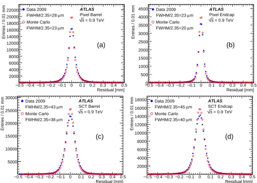
Unbiased x residuals from the silicon detectors are shown in Fig. 7, where x refers to the more precise local coordinate on the detector. Charged particles are selected to have pT> 2 GeV. The equivalent Gaussian width is extracted
from the full-width at half maximum. The width of the resulting distributions in data are within about 15% of those found in a simulation with no alignment errors, showing that the remaining impact on the residual widths from imperfect alignment in data is at the level of approximately 10-15 µm for the pixels and of 20 µm for the SCT. Residual [mm] −0.5 −0.4 −0.3 −0.2 −0.1 0 0.1 0.2 0.3 0.4 0.5 Entries / 0.01 mm 2000 4000 6000 8000 10000 12000 14000 16000 18000 20000 22000 ATLAS Pixel Barrel = 0.9 TeV s (a) Data 2009 m µ FWHM/2.35=28 Monte Carlo m µ FWHM/2.35=23 Residual [mm] −0.5 −0.4 −0.3 −0.2 −0.1 0 0.1 0.2 0.3 0.4 0.5 Entries / 0.01 mm 0 500 1000 1500 2000 2500 3000 3500 4000 4500 ATLAS Pixel Endcap = 0.9 TeV s (b) Data 2009 m µ FWHM/2.35=23 Monte Carlo m µ FWHM/2.35=20 Residual [mm] −0.5 −0.4 −0.3 −0.2 −0.1 0 0.1 0.2 0.3 0.4 0.5 Entries / 0.01 mm 5000 10000 15000 20000 25000 30000 ATLAS SCT Barrel = 0.9 TeV s (c) Data 2009 m µ FWHM/2.35=43 Monte Carlo m µ FWHM/2.35=38 Residual [mm] −0.5 −0.4 −0.3 −0.2 −0.1 0 0.1 0.2 0.3 0.4 0.5 Entries / 0.01 mm 2000 4000 6000 8000 10000 12000 14000 16000 18000 ATLAS SCT Endcap = 0.9 TeV s (d) Data 2009 m µ FWHM/2.35=45 Monte Carlo m µ FWHM/2.35=40
Figure 7: The distributions of the silicon detector unbiased residuals for (a) the pixel barrel, (b) the pixel end-cap, (c) the SCT barrel, (d) the SCT end-cap. The data are in solid circles, the simulation, which has a perfect alignment, is shown with open ones.
5.2
K
0SStudies
[MeV] π π m 400 450 500 550 600 650 700 750 800Entries / 2 MeV
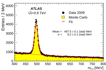
0 1000 2000 3000 4000 5000 6000 Data 2009 Monte Carlo Fit 0.1 (stat) MeV ± Mean = 497.5 0.1 (stat) MeV ± = 8.2 σ ATLAS =0.9 TeV s Figure 8: The K0Scandidate mass distribution using impact parameter and
life-time selections. The simulated signal and background are separately normalized to the data.
The momentum scale and resolution of the tracker, and energy loss with in, were all investigated by studying the K0
S to π+π −
decay. The reconstruction requires pairs of oppositely-charged particles compatible with coming from a common vertex. This vertex, in the transverse plane, must be more than 0.2 mm from the primary vertex. The cosine of the angle between the flight path relative to the primary vertex and the momentum vector of the candidate, cos θK, is
required to exceed 0.8. The invariant mass distribution, calculated assuming that both charged particles are pions is shown in Fig. 8. The simulated signal and background are separately normalized to the data, and the position and width of the K0
S mass peak are fitted using a Gaussian. The peak in data is at
mππ = 497.5 ± 0.1 MeV, in agreement with the PDG average [14].
In order to test the momentum scale and resolution of the detector the reconstructed pions in the simulation are adjusted by parameters µtr, which
scales the 1/pT, and σtr, a Gaussian smearing on µtr. The values of these
parameters which best fit the observed K0
S mass and width in the barrel region
are µtr= 1.0004 ± 0.0002 and σtr= 0.0040 ± 0.0015. Thus the momentum scale
for these barrel charged particles is known at better than the one per mille level, which is as expected from the accuracy of the solenoid magnet field-mapping performed before installation of the inner detector [15]. This, and subsequent K0
S studies, use a tighter cut of 0.99 on cos θK.
In the end-cap regions there is evidence for a degraded resolution, especially at low momentum. Charged particles with pT below 500 MeV require a σtr of
0.024±0.004 and 0.022±0.004 in the negative and positive end-caps, respectively, to match the data, suggesting some material is missing in the description of the end-caps. The momentum scale in the end-caps is compatible with the nominal
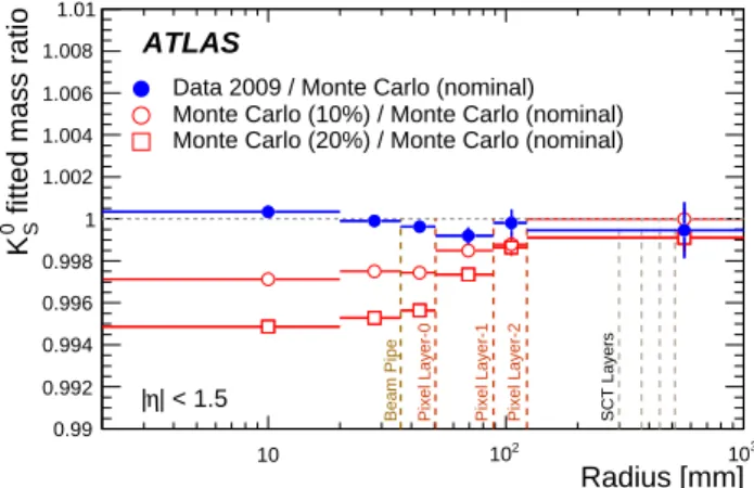
The KS0 peak was also used to investigate the amount of material in the
inner tracker as a function of radius. The mass reconstructed in data, divided by that found in simulation, is shown in Fig. 9 as a function of decay radius.
Radius [mm]
10 102 3
10
fitted mass ratio
0 S K 0.99 0.992 0.994 0.996 0.998 1 1.002 1.004 1.006 1.008 1.01
Beam Pipe Pixel Layer-0 Pixel Layer-1 Pixel Layer-2 SCT Layers
Data 2009 / Monte Carlo (nominal) Monte Carlo (10%) / Monte Carlo (nominal) Monte Carlo (20%) / Monte Carlo (nominal)
| < 1.5
η
| ATLAS
Figure 9: The fitted K0
Smass divided by the value found in nominal MC
simu-lation as a function of the reconstructed decay position. The filled circles show the data, and the open symbols are for simulation samples with approximately 10% and 20% more silicon tracker material added. The horizontal dotted line is to guide the eye.
Deviations of this ratio from unity would expose differences between the real detector and the model used for simulation. The results for special simulation samples with approximately 10% and 20% fractional increase in the radiation length of the silicon systems included by increasing the density of some of the support structures are also shown in Fig. 9. These results suggest that discrep-ancies of material between the data and the simulation must be significantly smaller than 10% of the material thickness in the inner silicon barrels.
5.3
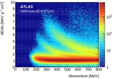
dE/dx and φ(1020) Identification
One feature of the Pixel tracking system is a time-over-threshold measurement for the signal which was used to extract the specific energy loss dE/dx. Tracks with more than one Pixel hit were studied and the mean dE/dx was found for each after the highest was removed to reduce the effect of Landau fluctuations. Figure 10 shows the distribution observed in the data. Bands corresponding to different particle species are clearly visible.
In the observation of φ → K+K−
identification of the K±
reduces the com-binatorial background. The identification of kaon candidates through dE/dx proceeds by finding the probability density functions of pions (ppion), kaons
(pkaon) and protons (pproton) in the simulation as a function of momentum and
dE/dx. This is done via fitting the observed value in simulation using a Gaus-sian function whose parameters are momentum dependent. The simulation models the data with an accuracy of about 10%.
The tracks used in the reconstruction of the φ meson must have more than one hit in the Pixel system and an impact parameter within 3σ of the primary vertex. The track fit was re-run using the kaon mass hypothesis for the energy
1 10 2 10 3 10 Momentum [MeV] 0 100 200 300 400 500 600 700 800 ] 2 cm -1 dE/dx [MeV g 0 1 2 3 4 5 6 7 8 9 10 ATLAS =0.9 TeV) s 2009 Data (
Figure 10: The dE/dx measured in data as a function of momentum. loss. The simulation shows that after re-fitting the kaon momenta are underesti-mated by up to 10 MeV and a corresponding correction is applied. This changes the reconstructed φ mass by approximately 0.3 MeV. All oppositely charged par-ticle pairs where both momenta, reconstructed under the kaon hypothesis, are below 800 MeV are considered.
[MeV] -K + K m 980 1000 1020 1040 1060 1080 1100 Entries / 2 MeV 0 100 200 300 400 500 980 1000 1020 1040 1060 1080 1100
Monte Carlo (signal) Monte Carlo (background) Data 2009 Fit ATLAS = 0.9 TeV s
Figure 11: The measured and simulated mass spectra of K+K−
pairs. The φ peak is fitted with a Breit-Wigner with a fixed width convoluted with a Gaussian. Both kaons must be identified through the dE/dx measurement.
Figure 11 shows the resulting mass distribution for the K+K−
candidate pairs, selected using charged particles with 200 < pT < 800 MeV and a kaon
dE/dx tag. The selection cuts were chosen to yield optimal signal significance on simulated events; a measure which was greatly improved using the dE/dx
The background and signal levels in the simulation were scaled independently to match the data. The fit allowed the mass and experimental resolution to vary, while keeping the natural width fixed to the PDG [14] average. The mass was found to be 1019.5±0.3 MeV, in agreement with the expected value. The fitted experimental resolution in data is 2.5±0.5 MeV and matches the 2.4±0.3 MeV found in Monte Carlo simulation.
5.4
Secondary Vertex Tagging
An important role of the tracking system is the identification of heavy flavour hadrons. There are several tagging algorithms developed in ATLAS. Some per-formance figures for two algorithms, the impact parameter and the secondary vertex tagging algorithm, are presented in the following.
The transverse impact parameter, d0, is a key variable for discriminating
tracks originating from displaced vertices from those originating from the pri-mary vertex. For studies of track impact parameters the d0 was calculated with
respect to a primary vertex which was fitted excluding that track in order to remove bias.
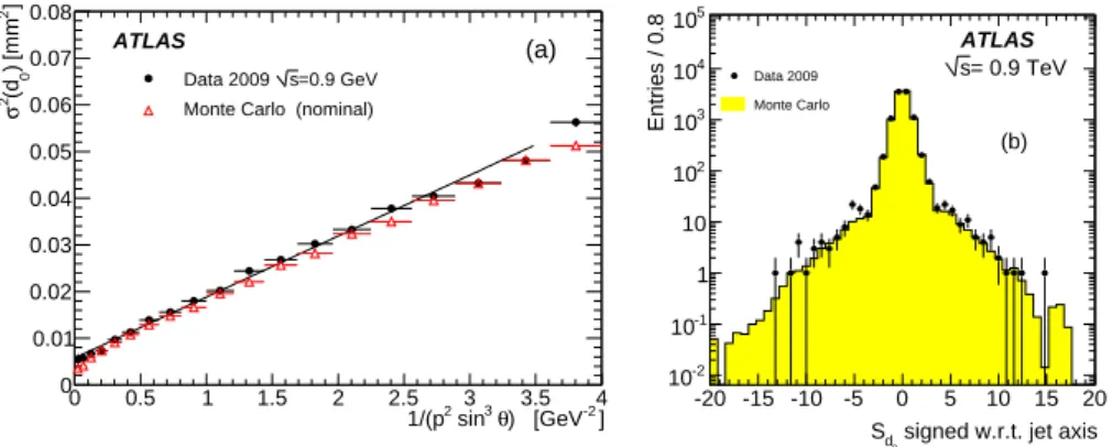
In order to study the effect of material on the d0resolution, Fig. 12(a) shows
σ2(d
0) versus 1/(p2sin3θ) for data and simulation using all selected charged
particle tracks. The quantity σ(d0) is determined by fitting the d0distribution
in each bin of 1/(p2sin3
θ) with a Gaussian within ±2σ(d0) about its mean. The
data lie approximately on a straight line, as is expected if the scattering material is on a cylinder and the match of the slope with the simulation implies a good description of the material of the inner detector. It should be noted that the intercept on the y axis has a contribution from the primary vertex resolution.
-2 ) [GeV ] θ 3 sin 2 1/(p 0 0.5 1 1.5 2 2.5 3 3.5 4 2 [mm ] ) 0 (d 2 σ 0 0.01 0.02 0.03 0.04 0.05 0.06 0.07 0.08 =0.9 GeV s Data 2009 Monte Carlo (nominal)
ATLAS (a)
signed w.r.t. jet axis
0 d S -20 -15 -10 -5 0 5 10 15 20 Entries / 0.8 -2 10 -1 10 1 10 2 10 3 10 4 10 5 10 = 0.9 TeV s Data 2009 Monte Carlo ATLAS (b)
Figure 12: (a) The variance of the d0 distribution as a function of 1/(p2sin3θ)
of the tracks for data (solid points) compared to the nominal simulation (open points). A straight line fit to the data points is also shown. (b) The lifetime-signed impact parameter significance.
The track selection for the b-tagging algorithms is designed to select well-measured particles and reject badly well-measured tracks, tracks from long-lived particles (K0
S, Λ and other hyperon decays), and particles arising from material
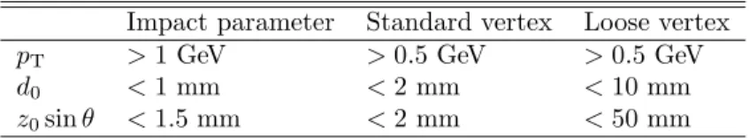
Table 2: Track selection criteria used for the impact parameter and secondary vertex tagging algorithms.
Impact parameter Standard vertex Loose vertex
pT > 1 GeV > 0.5 GeV > 0.5 GeV
d0 < 1 mm < 2 mm < 10 mm
z0sin θ < 1.5 mm < 2 mm < 50 mm
The track selection used by the impact parameter tagging algorithm is sum-marized in the first column of Table 2. Slightly different selections are used by the secondary vertex algorithm (second column of Table 2).
Calorimeter jets (see Section 7) are the reconstructed objects the tagging algorithms are typically applied to. Their direction is taken as estimator of the putative heavy flavour hadron direction. The impact parameter is then signed by whether the track perigee, relative to the jet direction, suggests a positive or negative flight distance. The distribution of the lifetime-signed impact param-eter significance for tracks in jets is shown in Fig. 12(b).
Reconstructing explicitly the secondary decay vertices of heavy flavour had-rons adds substantial tagging information. There are expected to be few b-quarks which can be tagged in this data set, so the algorithm was run with the standard as well as loose settings, as described in the second and third columns of Table 2, respectively. The loose setting selects vertices originating from K0 S
as well as from b-hadron decays whereas in the standard configuration any pair of tracks consistent with a K0
S, Λ or photon conversion is explicitly removed.
Secondary vertices are reconstructed in an inclusive way starting from two-track vertices which are merged into a common vertex. Tracks giving large χ2
contributions are then iteratively removed until the reconstructed vertex fulfils certain quality criteria.
The mass distribution of the resulting vertices for the loose configuration, assuming a pion mass for each track, is shown in Fig. 13.
Vertex mass [GeV] 0 0.5 1 1.5 2 2.5 3 Entries / 0.1 GeV -2 10 -1 10 1 10 ATLAS = 0.9 TeV s Data 2009 Monte Carlo
Figure 13: The vertex mass distribution for all secondary vertices with pos-itive decay length selected in data. The expectation from simulated events,
Running the algorithm in the standard configuration results in the recon-struction of 9 secondary vertices with positive decay length significance. This is in good agreement with the 8.9 ± 0.5(stat.) vertices expected from the same number of jets, 10 503, in non-diffractive minimum-bias simulation. The vertices reconstructed with the standard version of the tagging algorithm are predom-inantly those with higher masses as the low-mass region is dominated by K0 S
mesons.
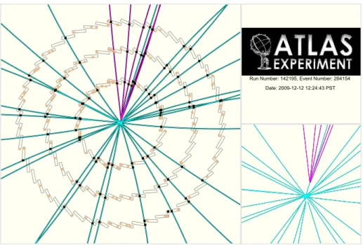
Figure 14: An event containing a secondary vertex selected by the secondary vertex algorithm. The pixel detector can be seen on the left and an expansion of the vertex region on the right. Unassociated hits, in a lighter colour, are predominantly due to unreconstructed particles such as those with transverse momenta below 0.5 GeV.
An event display of the highest-mass candidate is shown in Fig. 14. The secondary vertex consists of five tracks and has a mass of 2.5 GeV. The vertex is significantly displaced from the primary vertex, with a signed decay length significance L/σ(L) = 22. From the vertex mass, momentum and L a proper lifetime of 3.1 ps is estimated. The data was also tested by the impact-parameter based b-tagging algorithm and this jet is assigned a probability below 10−4 for
originating from a light quark jet.
5.5
Particle Identification using Transition Radiation
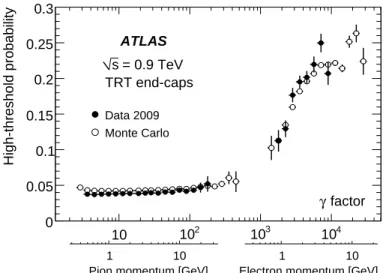
The TRT provides substantial discrimination between electrons and pions over the wide energy range between 1 and 200 GeV by utilizing transition radiation in foils and fibres. The readout discriminates at two thresholds, the lower set to register minimum-ionising particles and the higher intended for transition radiation (TR) photon interactions. The fraction of high-threshold TR hits as a
function of the relativistic γ factor is shown in Fig. 15 for particles in the forward region. This region is displayed because there are more conversion candidates and they have higher momenta than in the barrel.
factor γ 10 102 103 104 High-threshold probability 0 0.05 0.1 0.15 0.2 0.25 0.3 ATLAS = 0.9 TeV s TRT end-caps Data 2009 Monte Carlo
Pion momentum [GeV]
1 10
Electron momentum [GeV]
1 10
Figure 15: The fraction of high-threshold transition radiation hits on tracks as a function of the relativistic γ factor (see text for details).
The high-γ part of the distribution is constructed using electrons from pho-ton conversions while the low-γ component is made using charged particle tracks with a hit in the B-layer and treating them as pions. All tracks are required to have at least 20 hits in the TRT. The photon conversions are found similarly to those in Section 6.7 with at least one silicon hit, but the transition radiation electron identification was not applied to the electron that was being plotted. To ensure high purity (about 98%), the conversion candidates are also required to have a vertex more than 40 mm away from the beam axis. The pion sample excludes any photon conversion candidate tracks.
5.6
Tracking Efficiency for Level-2 Trigger
The L2 track trigger is one component of the HLT whose performance can be tested with current data. The trigger runs custom track reconstruction algo-rithms at L2, designed to produce fast and efficient tracking using all tracking subdetectors. Tracking information forms an integral part of many ATLAS triggers including electron, muon and tau signatures [16]. These use L1 infor-mation to specify a region of interest to examine. In the 2009 data there were few high-pT objects, so the results here are taken from a mode which searches
for tracks across the entire tracking detector and is intended for B-physics and beam-position determination at L2.
Offline tracks with |d0| < 1.5 mm and |z0| < 200 mm are matched to L2
tracks if they are within ∆R =p∆η2+ ∆φ2 < 0.1. The efficiency is defined
as the fraction of offline tracks which are matched and is shown in Fig. 16 as a function of the track pT.
[GeV] T Offline track p 1 2 3 4 5 6 7 8 9 10 L2 track ef ficie ncy [%] 0 20 40 60 80 100 Data 2009 Monte Carlo ATLAS = 0.9 TeV s
Figure 16: The efficiency for reconstruction of a L2 track candidate as a function of the pTof the matched offline track in data and Monte Carlo simulation. A
fit of the threshold curve is superimposed.
6
Electrons and Photons
The electron and photon reconstruction and identification algorithms used in ATLAS are designed to achieve a large background rejection and a high and uniform efficiency over the full acceptance of the detector for transverse ener-gies above 20 GeV. Using these algorithms on the 0.9 TeV data, a significant number of low-pTelectron and photon candidates were reconstructed. The
mea-surements provide a quantitative test of both the algorithms themselves and the reliability of the performance predictions in the transverse energy range from the reconstruction threshold of 2.5 GeV to about 10 GeV.
The electromagnetic calorimeter (EM) consists of the barrel (EMB) and two end-caps (EMEC). The barrel covers the pseudorapidity range |η| < 1.475; the end-cap calorimeters cover 1.375 < |η| < 3.2. In the forward direction energy measurements for both electromagnetic and hadronic showers are provided by the Forward Calorimeter (FCal) in the range 3.1 < |η| < 4.9. The hadronic calorimetry in the range |η| < 1.7 is provided by the scintillator-tile calorimeter (Tile). For 1.5 < |η| < 3.2 hadronic showers are measured by the hadronic end-caps (HEC), which use LAr with a copper absorber.
The e/γ algorithms make use of the fine segmentation of the EM calorimeter in both the lateral and longitudinal directions of the showers [1]. At high energy, most of the EM shower energy is collected in the second layer which has a lateral granularity of 0.025×0.025 in η×φ space. The first layer consists of finer-grained strips in the η-direction (with a coarser granularity in φ), which improves γ-π0 discrimination. A third layer measures the tails of very highly energetic EM
showers and helps in rejecting hadron showers. In the range |η| < 1.8 these three layers are complemented by a presampler layer placed in front with coarse granularity to correct for energy lost in the material before the calorimeter.
The algorithms also make use of the precise track reconstruction provided by the inner detector. The TRT also provides substantial discriminating power between electrons and pions over a wide energy range (between 1 and 200 GeV). The Pixel B-layer provides precision vertexing and significant rejection of photon conversions through the requirement of a track with a hit in this layer.
6.1
Electron and Photon Reconstruction
The basic algorithms for electron and photon reconstruction are described in detail in Ref. [16]. The first stage of the search for EM objects is to look for significant deposits in the EM calorimeter cells inside a sliding window as it is moved across the detector. The size of the sliding window cluster depends on the type of candidate (electron, unconverted or converted photon) and the location (barrel, end-caps). The cluster energy is calculated from the amplitudes observed in the cells of the three longitudinal layers of the EM calorimeter and of the presampler (where present). The calculation sums the weighted energies in these compartments, then takes into account several corrections for shower depth, lateral and longitudinal leakage, local modulation etc. The weights and correction coefficients were parameterized from beam-tests [1] and simulation.
Electrons are reconstructed from the clusters if there is a suitable match with a particle track of pT> 0.5 GeV. The best track is the one with an extrapolation
closest in (η, φ) to the cluster barycentre (the energy-weighted mean position) in the middle EM calorimeter layer. Similarly, photons are reconstructed from the clusters if there is no reconstructed track matched to the cluster (unconverted photon candidates) or if there is a reconstructed conversion vertex matched to the cluster (converted photon candidates). “Single track conversions” (identified via tracks lacking a hit in the B-layer) are also taken into account. First, electron candidates with a cluster |η| < 2.47 and photons with cluster |η| < 2.37 are selected and investigated (the cluster η is defined here as the barycentre of the cluster cells in the middle layer of the EM calorimeter). Electron and photon candidates in the EM calorimeter transition region 1.37 < |η| < 1.52 are not considered. At this stage, 879 electron and 1 694 photon candidates are reconstructed in the data with ET above 2.5 GeV.
6.2
Electron and Photon Identification
The isolated electron and photon identification algorithms rely on selections based on variables which provide good separation between electrons/photons and fake signatures from hadronic jets. These variables include information from the calorimeter and, in the case of electrons, tracker and combined calorime-ter/tracker information. There are three classes of electrons defined: loose, medium and tight, and two for photons: loose and tight. The selection criteria were optimized in bins of ET and η, separately for electrons, unconverted and
converted photons.
The loose selection criteria are based on the shower shape and are common to electrons and photons. For electrons, the medium requirements make use of the track information while in the tight ones the particle track selections are more stringent and use the particle identification capability of the TRT. For photons the tight selection criteria make full use of the EM calorimeter strip layer information, mainly to reject merged photon pairs from high energy π0’s.
In the following all reconstructed electron and photon candidates with cluster ET > 2.5 GeV at the sliding window level are considered.
6.3
Electron Candidates
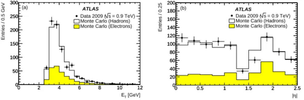
Figure 17 displays, for all of the 879 electron candidates from 384 186 events, the transverse energy and pseudorapidity spectra. Table 3 presents the percentage of these candidates which pass the successive selection criteria both for data and simulation. These criteria were not optimized for such low-energy electron candidates (see Section 6.2). Both Fig. 17 and Table 3 show similar behaviour in data and simulation. The remaining discrepancies in the first stages of back-ground rejection may be related to the small differences observed in shower variables (see Section 6.6.1 below). In Fig. 17(b) the drop in efficiency around |η| = 1.5 corresponds to the barrel/end-cap transition.
Table 3: The fraction of electron and photon candidates passing the different selection criteria, compared to those predicted by Monte Carlo (MC). Statistical error are quoted.
Electron candidates Photon candidates
Data (%) MC (%) Data (%) MC (%)
Loose 46.5±1.7 50.9±0.2 25.4±1.0 30.5±0.1
Medium 10.6±1.0 13.1±0.2 n.a. n.a.
Tight 2.3±0.5 2.4±0.1 4.1±0.5 6.6±0.1
In these figures the Monte Carlo prediction is sub-divided into its two main components: hadrons and real electrons. The latter is largely dominated by electrons from photon conversions, but also includes a small fraction (∼ 3%) of electrons from other sources, such as Dalitz decays, and an even smaller one (below 1%) of electrons from b, c → e decays. There are twenty electron candidates passing the tight selections in the data. Approximately 15% of such candidates in the Monte Carlo are from heavy flavour decays.
[GeV] T E 0 2 4 6 8 10 12 Entries / 0.5 GeV 0 50 100 150 200 250 300 0 2 4 6 8 10 12 0 50 100 150 200 250 300 = 0.9 TeV) s Data 2009 ( Monte Carlo (Hadrons) Monte Carlo (Electrons)
(a) ATLAS | η | 0 0.5 1 1.5 2 2.5 Entries / 0.25 0 20 40 60 80 100 120 140 160 180 200 0 0.5 1 1.5 2 2.5 0 20 40 60 80 100 120 140 160 180 200 = 0.9 TeV) s Data 2009 ( Monte Carlo (Hadrons) Monte Carlo (Electrons)
ATLAS
(b)
Figure 17: Distribution of cluster ET (a) and |η| (b) for all selected electron
candidates. The simulation is normalized to the number of data events.
6.4
Photon Candidates
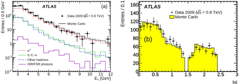
Transverse energy and pseudorapidity spectra for all 1 694 photon candidates are displayed in Fig. 18. Table 3 presents the percentage of photon candidates,
[GeV] T E 3 4 5 6 7 8 9 10 11 12 Entries / 0.5 GeV -2 10 -1 10 1 10 2 10 ATLAS (a) = 0.9 TeV) s Data 2009 ( Monte Carlo 0 π ω ’, η , η Other hadrons ISR/FSR photons | η | 0 0.5 1 1.5 2 2.5 3 Entries / 0.1 0 20 40 60 80 100 120 140 160 0 0.5 1 1.5 2 2.5 3 0 20 40 60 80 100 120 140 160 = 0.9 TeV) s Data 2009 ( Monte Carlo ATLAS (b)
Figure 18: Cluster ET (a) and |η| (b) for all selected photon candidates. The
simulation is normalized to the number of data events.
as a function of the selection level applied. Of the selected candidates, 14% are reconstructed as converted photons and almost all of these, ∼ 98%, are also selected as electron candidates.
The Monte Carlo prediction is sub-divided in this case into four components of decreasing importance: approximately 71% of the candidates correspond to photons from π0 decay, whereas ∼ 14% are from η, η′
or ω decays into pho-tons; ∼ 14% are from other hadrons with complex decay processes and particles interacting in the tracker material. At these energies, only a very small fraction, ∼ 1%, of all photon candidates are expected to be primary products of the hard scattering.
6.5
First-level Electron and Photon Trigger Performance
The L1 e/γ selection algorithm searches for narrow, high-ET electromagnetic
showers and does not separate electrons from photons. The primitives for this algorithm are towers which sum the transverse energies of all electromagnetic calorimeter cells in ∆η × ∆φ = 0.1 × 0.1. The trigger examines adjacent pairs of towers and tests their total energy against several trigger thresholds. Isolation requirements were not yet employed. The lowest threshold e/γ trigger for the 2009 data-taking period required a transverse energy of at least 4 GeV.
Clusters consistent with originating from an electron or photon are selected by requiring at least 30% of the cluster energy to be deposited in the second layer of the electromagnetic calorimeter, where the maximum of an electromagnetic shower is expected. The selected e/γ candidates are matched to L1 clusters in η and φ by requiring ∆R < 0.15. The efficiency is then calculated from the fraction of reconstructed clusters which have a matching L1 cluster.
The resulting L1 trigger efficiency for the lowest threshold component is shown in Fig. 19. The sharpness of the efficiency turn-on curve around threshold agrees with the Monte Carlo expectation. Low energy reconstructed clusters occasionally fire the trigger, especially when the coarser granularity used at L1 merges two separate offline clusters.
[GeV] Raw T E 0 2 4 6 8 10 12 14 16 L1 efficiency 0 0.2 0.4 0.6 0.8 1 ATLAS = 0.9 TeV) s Data 2009 ( Monte Carlo
Figure 19: Efficiency for the lowest threshold L1 electromagnetic trigger, a nominal 4 GeV, as a function of the uncalibrated offline cluster transverse energy. The turn-on is shown for data (solid triangles) and non-diffractive minimum-bias simulation (open circles).
0 f -0.2 0 0.2 0.4 0.6 0.8 1 Entries / 0.02 -2 10 -1 10 1 10 2 10 3 10 4 10 5 10 -0.2 0 0.2 0.4 0.6 0.8 1 -2 10 -1 10 1 10 2 10 3 10 4 10 5 10 = 0.9TeV) s Data 2009 ( Monte Carlo (a) ATLAS 1 f -0.2 0 0.2 0.4 0.6 0.8 1 Entries / 0.02 0 20 40 60 80 100 120 140 160 180 200 -0.20 0 0.2 0.4 0.6 0.8 1 20 40 60 80 100 120 140 160 180 200 = 0.9TeV) s Data 2009 ( Monte Carlo ATLAS (b) 2 f -0.2 0 0.2 0.4 0.6 0.8 1 Entries / 0.02 0 20 40 60 80 100 120 140 -0.20 0 0.2 0.4 0.6 0.8 1 20 40 60 80 100 120 140 = 0.9TeV) s Data 2009 ( Monte Carlo ATLAS (c) 3 f -0.2 0 0.2 0.4 0.6 0.8 1 Entries / 0.02 -2 10 -1 10 1 10 2 10 3 10 4 10 5 10 -0.2 0 0.2 0.4 0.6 0.8 1 -2 10 -1 10 1 10 2 10 3 10 4 10 5 10 = 0.9TeV) s Data 2009 ( Monte Carlo ATLAS (d)
Figure 20: Fraction of energy deposited by photon candidates with ET >
2.5 GeV in each layer of the electromagnetic calorimeter for data and simu-lation. These fractions are labelled as (a) f0for the presampler layer, (b) f1for
the strip layer, (c) f2 for the middle layer and (d) f3for the back layer.
Frac-tions can be negative due to noise fluctuaFrac-tions. The simulation is normalized to the number of data events.
6.6
Electron and Photon Identification Variables
6.6.1 Calorimeter VariablesIn this section, various calorimeter-based quantities are displayed for the photon candidates. These are preferred to the similar electron distributions because of the higher purity.
Figure 20 illustrates the longitudinal development of the shower in the suc-cessive layers of the EM calorimeter, based on the measured layer energies before corrections are applied. For the observed photon candidates, which in simulation are predominantly from π0decays, the energy is deposited in earlier calorimeter
layers than typical for high energy photons. In the presampler part, the simu-lation points are higher than the data for fractions above 0.6. This is at least in part because the presampler simulation does not describe the recombination of electron-positron pairs by highly ionizing hadrons or nuclear fragments that lower the LAr response, an effect which is included in the accordion calorimeter simulation. This feature also explains the observed disagreement in the first bins for the fractions in the other layers, since the various fractions are correlated.
Several variables are used to quantify the lateral development of the shower. From these, the distribution of w2, the shower width measured in the second
layer of the EM calorimeter, is shown in Fig. 21(a). The shower width w2 is
slightly larger in the data. Preliminary studies show that including the cross-talk between neighbouring middle layer cells (∼ 0.5%) [17] in the simulation explains part of the observed difference.
The distribution of two variables used for π0/γ separation in the tight photon
selection, Eratio and ws3, are shown in Figs. 21(b) and 21(c). Eratio is the
difference of the highest and second highest strip energies, divided by their sum. ws3 is the shower width measured in three strips around the maximum
energy strip. For this variable the data show a slightly wider profile than the simulation, although in this case the simulation already includes the measured cross-talk. In general, all the shower shape variables show good agreement between data and simulation.
6.6.2 Tracking and Track-Cluster Matching Variables
Electron and converted photon identification rely heavily on tracking perfor-mance. Figure 22 illustrates two of the track-calorimeter matching variables used in the identification of electron candidates in data and simulation. For simulation, hadrons and real electrons are shown separately. Fig. 22(a) shows the difference in η, ∆η1, between the track extrapolated to the strip layer of
the EM calorimeter and the barycentre of the cell energies in this layer. Fig-ure 22(b) shows the difference in azimuth, ∆φ2, between the track extrapolated
to the middle layer of the EM calorimeter and the barycentre of the cell energies in this layer. This variable is signed by the charge of the particle to account for the position of any radiated photons with respect to the track curvature, and an asymmetric cut is applied in the selection. The asymmetric tails at large negative values of ∆φ2 are more pronounced for the electrons than for the
hadrons.
Figure 23 shows a comparison of four of the tracking variables between data and simulation for all electron candidates. Figures 23(a) and 23(b) show the
[cell] 2 w 0 0.1 0.2 0.3 0.4 0.5 0.6 0.7 0.8 Entries / 0.04 0 100 200 300 400 500 0 0.1 0.2 0.3 0.4 0.5 0.6 0.7 0.8 0 100 200 300 400 500 = 0.9TeV) s Data 2009 ( Monte Carlo ATLAS (a) ratio E 0 0.2 0.4 0.6 0.8 1 Entries / 0.02 0 20 40 60 80 100 120 140 160 180 0 0.2 0.4 0.6 0.8 1 0 20 40 60 80 100 120 140 160 180 ATLAS = 0.9TeV) s Data 2009 ( Monte Carlo (b) [cell] s3 w 0 0.1 0.2 0.3 0.4 0.5 0.6 0.7 0.8 0.9 Entries / 0.02 0 50 100 150 200 250 0 0.1 0.2 0.3 0.4 0.5 0.6 0.7 0.8 0.9 0 50 100 150 200 250 = 0.9TeV) s Data 2009 ( Monte Carlo ATLAS (c)
Figure 21: Distributions of calorimeter variables compared between data and simulation for all photon candidates with pT above 2.5 GeV. Shown are the
shower width in the middle layer of the EM calorimeter, w2(a), and the variables
Eratio (b) and ws3 (c), which characterize the shower shape in the first (strips)
EM layer. The simulation is normalized to the number of data events.
1 η ∆ -0.1 -0.05 0 0.05 0.1 Entries / 0.005 0 50 100 150 200 250 -0.10 0 0.1 50 100 150 200 250 = 0.9 TeV) s Data 2009 ( Monte Carlo (Hadrons) Monte Carlo (Electrons) ATLAS (a) 2 φ[rad] ∆ -0.1 -0.05 0 0.05 Entries / 0.01 0 50 100 150 200 250 300 350 -0.10 -0.05 0 0.05 50 100 150 200 250 300 350 = 0.9 TeV) s Data 2009 ( Monte Carlo (Hadrons) Monte Carlo (Electrons) ATLAS (b)
Figure 22: Distributions of track-calorimeter matching variables for all electron candidates compared between data and simulation. (a) shows the difference in η in the first calorimeter layer (see Section 6.6.2) and (b) shows the match in charge-signed-φ in the second. The simulation is normalized to the number of data events.
Number of pixel hits 0 2 4 6 8 10 Entries / 1.0 0 50 100 150 200 250 300 350 400 0 2 4 6 8 10 0 50 100 150 200 250 300 350 400 = 0.9 TeV) s Data 2009 ( Monte Carlo (Hadrons) Monte Carlo (Electrons) ATLAS (a) Number of SCT hits 0 2 4 6 8 10 12 14 Entries / 1.0 0 50 100 150 200 250 300 350 400 450 500 0 2 4 6 8 10 12 14 0 50 100 150 200 250 300 350 400 450 500 = 0.9 TeV) s Data 2009 ( Monte Carlo (Hadrons) Monte Carlo (Electrons) ATLAS (b)
Fraction of high-threshold TRT hits
0 0.1 0.2 0.3 0.4 0.5 Entries / 0.025 0 20 40 60 80 100 120 140 160 180 200 0 0.1 0.2 0.3 0.4 0.5 0 20 40 60 80 100 120 140 160 180 200 = 0.9 TeV) s Data 2009 ( Monte Carlo (Hadrons) Monte Carlo (Electrons) ATLAS (c) [mm] 0 d -1.5 -1 -0.5 0 0.5 1 1.5 Entries / 0.05 1 10 2 10 3 10 4 10 -1.51 -1 -0.5 0 0.5 1 1.5 10 2 10 3 10 4 10 ATLAS (d) = 0.9 TeV) s Data 2009 ( Monte Carlo (Hadrons) Monte Carlo (Electrons)
Figure 23: Distributions of tracking variables for all electron candidates com-pared between data and simulation. The number of Pixel (a) and SCT (b) hits on the electron tracks are shown, the fraction of high-threshold TRT hits for candidates with |η| < 2.0 and with a total number of TRT hits larger than ten (c), and the transverse impact parameter, d0, with respect to the
recon-structed primary vertex (d). The simulation is normalized to the number of data events.
fraction of high-threshold TRT hits belonging to the track for electron candi-dates with |η| < 2.0 and with a total number of TRT hits larger than ten is shown in Fig. 23(c). At these low energies the transition radiation yield of elec-trons is not optimal and yet a very clear difference can be seen between the distributions expected for hadrons and for electrons from conversions. Finally, Fig. 23(d) shows the distribution of the transverse impact parameter, d0, of
the electron track with respect to the reconstructed primary vertex position in the transverse plane; whereas the hadrons in the simulation display a distri-bution peaked around zero with a resolution of ∼ 100 µm, the electrons from conversions have large impact parameters. The agreement between data and simulation is good, despite the complications expected at these low energies due to material effects and track reconstruction inefficiencies.
E/p 0 0.5 1 1.5 2 2.5 3 3.5 4 4.5 5 Entries / 0.25 0 50 100 150 200 250 = 0.9 TeV) s Data 2009 ( Monte Carlo (Hadrons) Monte Carlo (Electrons) Monte Carlo
Conversions with Si hits ATLAS (a) E/p 0 0.5 1 1.5 2 2.5 3 3.5 4 4.5 5 Entries / 0.5 10 20 30 40 50 60 70 80 ATLAS (b) = 0.9 TeV ) s Data 2009 ( Data: 2009
(all tracks with Si hits) Monte Carlo Monte Carlo (all tracks with Si hits)
Figure 24: Ratio, E/p, between cluster energy and particle track momentum (a) for electron candidates and (b) for electrons from converted photons. In each case candidates with pTabove 2.5 GeV in the calorimeter are shown. Sub-figure
(a) is dominated by real electrons. The simulation is normalized to the number of data events.
Figure 24(a) shows the distribution of the ratio E/p of cluster energy in the calorimeter to track momentum for all electron candidates and for data and simulation. Electrons from conversions have a broad E/p distribution as their shortened tracks have a large momentum error. The hadron component peaks at values near unity: this behaviour, due to the selection bias for these hadrons, is also observed in the simulation. In a similar fashion, Fig. 24(b) shows the E/p ratio of the reconstructed converted photon candidates, where the converted photon momentum is estimated from the combination of the par-ticle momenta for double-track conversions and from the parpar-ticle momentum measurement available for single-track conversions. Approximately 20% of the converted photon candidates are reconstructed as single-track conversions in this kinematic regime. Both the electron dominated and the hadron dominated distributions show good agrement with the simulation.
6.6.3 Use of the TRT for Electron Identification
As already discussed in Section 6.3, the electron candidate data sample is ex-pected to consist predominantly of two components: charged hadrons
misre-constructed as electrons and electrons from photon conversions. These two components can be separated by using the measured fraction of high-threshold TRT hits on the electron tracks (see Fig. 23(c)). To perform such a measure-ment, the electron candidates are required to lie within the TRT acceptance, i.e. |η| < 2.0, and to have a reconstructed track with a total of at least ten TRT hits.
The distribution of the fraction of high threshold hits has been fitted in 20 bins between 0 and 0.5 to extract the number of hadrons and electrons observed in the data. This relies upon the modelling of the response of the TRT to electrons and pions in the simulation. The sample of electron candidates considered here is predicted to contain 494±26 electron candidates which are actually hadronic fakes and 226±21 genuine electrons.
Two examples of comparisons between the shapes of variables extracted for each of the two components, using the method described above (on each bin individually), and the shapes predicted for each component are shown in Figs. 25 and 26, respectively, for two of the most sensitive variables: the fraction of the cluster energy measured in the strip layer and the ratio E/p. The E/p distribution for electrons in both data and simulation shows a peak close to unity and a tail at large values from bremsstrahlung losses in the tracker material. The error estimates in these de-convolved plots come from toy Monte Carlo trials and their size reflects the power of the TRT detector for electron identification. The rates of electrons and hadrons and the relevant distributions agree with the Monte Carlo simulation for each species illustrating the quality of the simulation modelling. 1 f 0 0.1 0.2 0.3 0.4 0.5 0.6 0.7 0.8 0.9 1 Entries / 0.04 0 10 20 30 40 50 = 0.9 TeV) s Data 2009 ( Monte Carlo ATLAS (a) Electrons 1 f 0 0.1 0.2 0.3 0.4 0.5 0.6 0.7 0.8 0.9 1 Entries / 0.04 0 50 100 150 200 = 0.9 TeV) s Data 2009 ( Monte Carlo ATLAS (b) Hadrons
Figure 25: Distribution of the energy fraction in the strip layer of the EM calorimeter as extracted from data compared to the truth from simula-tion. The results are shown for both components of the electron candidates: electrons from conversions (a) and hadrons (b). The simulation is normalized to the number of data events.
6.7
Photon Conversions
An accurate and high-granularity map of the inner detector material is nec-essary for a precise reconstruction of high-energy photons and electrons. The location of the conversion vertex can be used as a tool to map the position and amount of material of the inner detector. In the following, photon conversions are selected using only information from the inner detector, enabling the use of very low momentum particle track pairs. In addition, conversions give a source
E/p 0 0.5 1 1.5 2 2.5 3 3.5 4 4.5 5 Entries / 0.2 0 10 20 30 40 50 = 0.9 TeV) s Data 2009 ( Monte Carlo ATLAS (a) Electrons E/p 0 0.5 1 1.5 2 2.5 3 3.5 4 4.5 5 Entries / 0.2 20 40 60 80 100 120 140 160 180 = 0.9 TeV) s Data 2009 ( Monte Carlo ATLAS (b) Hadrons
Figure 26: Distribution of the E/p as extracted from data compared to the truth from simulation. The results are shown for both components of the electron candidates: electrons from conversions (a) and hadrons (b). The simulation is normalized to the number of data events.
The conversion reconstruction algorithm is described in detail elsewhere [16]. In the following, the basic steps of the algorithm are recalled together with an updated list of selection criteria. The algorithm begins by selecting single particle tracks with transverse momentum pT> 500 MeV. These tracks must
have a probability of being an electron of more than 10%, calculated using the particle identification capability of the TRT, see Section 5.5.
Conversion candidates are then created by pairing oppositely charged par-ticle tracks. The tracks are further required to be close in space and to have a small opening angle. The selected particle track pairs are then fitted to a common vertex with the constraint that they be parallel at the vertex. The final set of conversion candidates is selected based on the quality of the vertex fit which must have χ2 smaller than 50.
The tracks used for the reconstruction of conversions may be stand-alone TRT tracks, or they may include silicon hits. In the data, 3 662 vertices, 6.7% of the total, have two tracks with silicon information, to be compared with 10.4% in the simulation. This class of vertices have much less background than the total and the following results are drawn from them. Some properties of the candidates in data and Monte Carlo simulation are shown in Fig. 27. Given the complexity of the reconstruction of converted photons and the impact of bremsstrahlung of the electrons in the tracker material, the consistency between the data and the simulation for the selection variables is good.
To measure the inner detector material the selection requirements are tight-ened to >90% TR electron probability and vertex χ2< 5.
Figure 28 shows the location in radius and η of conversion vertices. The simulation was normalized to the same number of conversions as in the data and the agreement in shape is satisfactory.
The amount of material, in multiples of the radiation length X0, that the
photons traverse can be calculated from the fraction of photon conversions seen in it given the reconstruction efficiency. The combinatorial background and the error in determining the conversion radius must be accounted for. To remove the dependence on the absolute flux of photons and the overall reconstruction efficiency, the rate is normalized to that seen in a well-understood reference ma-terial volume, which is chosen to be the beam pipe. As shown in Fig. 28, there were only 9 conversions in this reference volume and so the absolute material
) θ (1/tan ∆ -0.3 -0.2 -0.1 0 0.1 0.2 0.3 Entries / 0.02 0 100 200 300 400 500 600 700 ) θ (1/tan ∆ -0.3 -0.2 -0.1 0 0.1 0.2 0.3 Entries / 0.02 0 100 200 300 400 500 600 700 Data 2009 Monte Carlo (true conversions) Monte Carlo ATLAS = 0.9 TeV s (a) dr [mm] 0 1 2 3 4 5 6 7 8 9 10 Entries / 0.4 mm 1 10 2 10 3 10 dr [mm] 0 1 2 3 4 5 6 7 8 9 10 Entries / 0.4 mm 1 10 2 10 3 10 Data 2009 Monte Carlo (true conversions) Monte Carlo ATLAS = 0.9 TeV s (b)
Figure 27: Comparison between converted photon candidates, for which both tracks have silicon hits, in data and non-diffractive minimum-bias Monte Carlo simulation. (a) Opening angle in the rz plane between the two tracks (∆(1/tanθ)); (b) 3D distance of closest approach between the two tracks, dr. The distributions are normalized to the same number of conversion candidates in data and Monte Carlo simulation.
determination has errors of at least 30%. The agreement between data and Monte Carlo is presented in Table 4.
6.8
Reconstruction of π
0and η Mesons
For the analysis presented in this section, cells from the four layers are com-bined to form a cluster of size ∆η × ∆φ = 0.075 × 0.125, which corresponds to an area of 3 × 5 cells in the middle layer of the EM calorimeter. The EM cell clusters are reconstructed with a seed cell threshold |Ecell| = 4σ (where σ
corresponds to the electronic noise in the cell) and with a cluster transverse energy ET > 300 MeV [16]. These clusters are used as photon candidates for
π0 and η reconstruction.
The standard parameterization of energy response discussed in Section 6.1 was performed for photons with ET > 5 GeV. For the present study a dedicated
parameterization was extracted from the minimum-bias simulation sample using low-energy photons coming only from π0s.
6.8.1 Extraction of π0
→γγ Signal
In order to extract the π0 signal from the combinatorial background, well
mea-sured photons were selected inside an acceptance of |η| < 2.37, excluding a transition region 1.37 < |η| < 1.52. The fraction of energy in the first layer, E1/(E1+ E2+ E3), was required to be larger than 0.1 and the clusters were
required to have a transverse energy, ET, above 400 MeV.
All pairs of photons with ppairT > 900 MeV are selected. There are about 8 × 10⁵ of these in the data.
R [mm] 0 50 100 150 200 250 300 350 400 Entries / 8 mm 0 5 10 15 20 25 30 35 40 R [mm] 0 50 100 150 200 250 300 350 400 Entries / 8 mm 0 5 10 15 20 25 30 35 40 = 0.9 TeV) s Data 2009 ( (conversion candidates) Monte Carlo (true conversions) Monte Carlo
(true Dalitz decays) Monte Carlo ATLAS (a) η -2.5 -2 -1.5 -1 -0.5 0 0.5 1 1.5 2 2.5 Entries / 0.2 0 5 10 15 20 25 30 35 η -2.5 -2 -1.5 -1 -0.5 0 0.5 1 1.5 2 2.5 Entries / 0.2 0 5 10 15 20 25 30 35 = 0.9 TeV) s Data 2009 ( (conversion candidates) Monte Carlo (true conversions) Monte Carlo ATLAS (b)
Figure 28: Distribution of conversion candidate radius, (a), and η, (b). The points show the distribution for data; the open histograms, the total from the Monte Carlo simulation and the filled component shows the expected contri-bution of true photon conversions. The contricontri-bution from the Dalitz decays of neutral mesons is shown in sub-figure (a). The Monte Carlo simulation is nor-malized to number of conversion candidates in the data, although in subsequent analysis normalization is to the number in the beam pipe.
6.8.2 π0
Mass Fit
The invariant mass distribution of the photon pairs is shown in Fig. 29 for both data and Monte Carlo. The diphoton mass distribution is fitted using a maximum-likelihood fit. The signal is described by the sum of a Gaussian and a “Crystal-Ball function” [18], which are required to have the same mean. The combinatorial background is described with a 4thorder Chebyshev polynomial.
The parameters of the signal and the background normalization are varied in the fit to the data, while the parameters of the polynomial were extracted from the Monte Carlo.
50 100 150 200 250 300 350 400 450 500 0 1000 2000 3000 4000 5000 6000 [MeV] γ γ m Entri e s / 10 MeV ATLAS signals) η / 0 π Monte Carlo ( Monte Carlo (background)
= 0.9 TeV) s Data 2009 (
Fit to data
Background component of the fit
(a) [MeV] -e + e γ Calibrated m 0 50 100 150 200 250 300 350 400 450 500 Events / 25 MeV 0 5 10 15 20 25 30 35 0 50 100 150 200 250 300 350 400 450 500 0 5 10 15 20 25 30 35 Data 2009 (s=0.9 TeV) Monte Carlo (b) ATLAS
Figure 29: (a) Diphoton invariant mass distribution for the π0 selection for
data and Monte Carlo. The Monte Carlo is normalized to the same number of entries as the data. (b) Invariant mass distribution from one converted and one unconverted photon. The data are represented by points and the Monte Carlo simulations are shown as histograms.
Table 4: Nreco is the number of reconstructed conversions in each layer, and
X/X0data and X/X0MC represent the amount of material in the different
volumes estimated from data and Monte Carlo, normalized by the number of reconstructed converted photons in the beam pipe, whose material is assumed to be correct. The normalization introduces an additional statistical uncertainty of 30% on X/X0data. Nreco XX0data X X0MC Beam pipe 9 0.00655 0.00655 Pixel B-layer 46 0.030 ± 0.004 0.032 Pixel layer 1 65 0.035 ± 0.004 0.027 Pixel layer 2 55 0.025 ± 0.003 0.023 SCT layer 1 25 0.020 ± 0.004 0.016
The fitted π0 mass is 134.0±0.8 MeV for the data and 132.9±0.2 MeV for
the Monte Carlo where the errors are statistical only. The mass resolution in the data is 24.0 MeV, to be compared with 25.2 MeV in the simulation, and the number of π0’s is (1.34 ± 0.02) × 104. This fit is sensitive to the modelling of
the background shape near the π0 mass. Varying the background shape under
the peak leads to a differences of up to 1% for the fitted π0 mass, up to 10%
for the fitted π0 mass resolution and up to 20% for the fitted total number of
signal events.
The 1% agreement of energy scale between data and Monte Carlo is well within the 2 - 3% uncertainty on the energy scale transported from test-beam data analysis. The 1.5% discrepancy of the mass found in Monte Carlo with respect to the PDG nominal π0 mass is consistent with the accuracy (as
evalu-ated with simulation) of the cluster calibration procedure used for the low-energy photons, and the 1% uncertainty arising from the background modelling.
The converted photons reconstructed in Section 6.7 can also be used to search for the π0. This is done here using one photon reconstructed in the
calorime-ter, with a track veto applied and one conversion candidate. The conversion candidates are required to have four silicon hits on both tracks and must be in the same hemisphere as the calorimeter cluster. Figure 29(b) shows the γe+e−
mass spectrum; the π0 peak is clearly visible.
The uniformity of the EM calorimeter response was studied in ten η bins, where both photons are in the same bin. The diphoton mass distribution in each η bin is fitted separately with the background shape constrained from simulation. The reconstructed π0mass is constant within 3% for both data and Monte Carlo for all η bins, and the ratio of data to Monte Carlo is consistent within the 2% statistical uncertainties.
6.8.3 Extraction of the η → γγ Signal
The number of η → γγ events is expected to be one order of magnitude smaller than π0→ γγ in the minimum-bias event sample. Therefore, the combinatorial