Applying high performance computing to early fusion video action recognition

Applying High Performance Computing to Early

Fusion Video Action Recognition

by

Matthew S. Hutchinson

Submitted to the Department of Electrical Engineering and Computer

Science

in partial fulfillment of the requirements for the degree of

Master of Engineering in Electrical Engineering and Computer Science

at the

MASSACHUSETTS INSTITUTE OF TECHNOLOGY

May 2020

c

○ 2020 Massachusetts Institute of Technology. All rights reserved.

Author . . . .

Department of Electrical Engineering and Computer Science

May 12, 2020

Certified by . . . .

Charles E. Leiserson

Edwin Sibley Webster Professor of Computer Science and Engineering

Thesis Supervisor

May 12, 2020

Certified by . . . .

Vijay Gadepally

MIT Lincoln Laboratory Senior Scientist

Thesis Supervisor

May 12, 2020

Accepted by . . . .

Katrina LaCurts

Chair, Master of Engineering Thesis Committee

Applying High Performance Computing to Early Fusion Video

Action Recognition

by

Matthew S. Hutchinson

Submitted to the Department of Electrical Engineering and Computer Science on May 12, 2020, in partial fulfillment of the

requirements for the degree of

Master of Engineering in Electrical Engineering and Computer Science

Abstract

Over the past few years, there has been significant interest in video action recognition systems and models. However, direct comparison of accuracy and computational per-formance results remain clouded by differing training environments, hardware speci-fications, hyperparameters, pipelines, and inference methods. Additionally, the liter-ature demonstrates a fixedness on late fusion approaches to audio-video multimodal problems. This project provides a side-by-side comparison of several 2-Dimensional Convolutional Neural Network (2D-CNN) video action recognition approaches and investigates the effectiveness and efficiency of new audio-video early fusion, slicing, and sampling methods. Model accuracy is evaluated using standard Top-1 and Top-5 metrics in addition to novel p-ROC metrics, and this project demonstrates the useful-ness of the latter. Computational performance is measured via total training time and training time per epoch on a variety of high-performance computing (HPC) training configurations.

Thesis Supervisor: Charles E. Leiserson

Title: Edwin Sibley Webster Professor of Computer Science and Engineering

Thesis Supervisor: Vijay Gadepally

Acknowledgments

These are wild times, and I never expected my M.Eng. conclusion to be like this. There are many people to thank for everything that has made this research and my education possible even in these trying times.

I would first like to thank my parents, Scott and Lynn Hutchinson for everything they have done to help me and sustain me. They were instrumental in helping push my education forward through high school and onto MIT. While at MIT, they continued to support me in many ways–financially, logistically, and emotionally.

Second, I would like to thank my supervisor, Dr. Vijay Gadepally. Dr. Gadepally helped me find an interesting project and avenue of research. He has always been helpful in refining problems, bouncing ideas around, and keeping me on track. I appreciate how he finds time to meet with me even amid his busy schedule.

Third, I would like to thank my thesis advisor, Professor Charles Leiserson. Pro-fessor Leiserson oversaw my research and allowed me conduct much of it through MIT Lincoln Laboratory Supercomputing Center (LLSC) via the VI-A Program.

I would also like to thank everyone else who made this research and education possible. The entire LLSC team helped answering my questions, providing awesome computational resources, making the research process enjoyable, and letting me camp out in their training room often. I will miss Wednesday afternoon tea. My friends also helped me get through these five years. MIT is a tough place with seemingly endless work, but it’s my friends that constantly found ways to make it fun. Additionally, countless MIT professors, staff, and administrators made the MIT experience unfor-gettable. I will wear my Brass Rat proud.

DISTRIBUTION STATEMENT A. Approved for public release. Distribution is unlim-ited. This material is based upon work supported by the Under Secretary of Defense for Research and Engineering under Air Force Contract No. FA8702-15-D-0001. Any opin-ions, findings, conclusions or recommendations expressed in this material are those of the author(s) and do not necessarily reflect the views of the Under Secretary of Defense for Research and Engineering.

Contents

1 Introduction 17

1.1 Video Action Recognition . . . 17

1.2 Modality Fusion . . . 19

1.3 High Performance Computing . . . 21

1.4 Training Pipeline . . . 22

1.5 Project Overview . . . 23

2 Background, Related Work, and Model Assessment 25 2.1 Action Recognition Datasets . . . 25

2.2 Machine Learning for Action Recognition . . . 27

2.3 Moments in Time . . . 30

2.4 Model Assessment Techniques . . . 32

3 Comparison Study 37 3.1 Initial Comparison . . . 37

3.1.1 Experimental Design . . . 38

3.1.2 Accuracy Performance Results . . . 39

3.1.3 Computational Performance Results . . . 40

3.2 Expanded Comparison . . . 42

3.2.1 Experimental Design . . . 42

3.2.2 Accuracy Performance Results . . . 43

3.2.3 Computational Performance Results . . . 44

4 Exploration of Video Slicing and Sampling 47

4.1 Experimental Design . . . 48

4.2 Accuracy Performance Results . . . 51

4.3 Computational Performance Results . . . 53

4.4 Discussion and Conclusions . . . 53

5 Experimentation with Early Fusion 55 5.1 Audio Representations . . . 55

5.2 Early Fusion Methods . . . 57

5.3 10-Class Experiment . . . 58

5.3.1 Experimental Design . . . 58

5.3.2 Accuracy Performance Results . . . 60

5.3.3 Computational Performance Results . . . 61

5.4 339-Class Experiment . . . 61

5.4.1 Experimental Design . . . 62

5.4.2 Accuracy Performance Results . . . 64

5.4.3 Computational Performance Results . . . 65

5.5 Discussion and Conclusions . . . 67

6 Conclusion 69

A Accuracy Performance Tables and Additional Figures 73

B Computational Performance Tables and Additional Figures 79

List of Figures

1-1 Example action recognition categories and video screenshots from the Moments in Time dataset [54]. . . 18 1-2 Generic early fusion architecture (adapted from [68]). Multi-modal

features are extracted and fused prior to being used as input to a supervised learner. . . 20 1-3 Generic late fusion architecture (adapted from [68]). Multi-modal

fea-tures are extracted and fed as inputs to separate supervised learned. The outputs of those learners are fused and fed as inputs to another supervised learner which typically consists of only a few dense layers to do classification and end with softmax output. . . 20 1-4 Overview of the Training Pipeline. . . 22

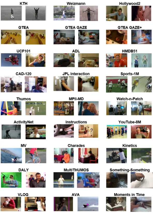
2-1 Action Recognition Dataset Zoo. Two screenshots are taken from sep-arate videos in each of the labeled datasets, giving a glimpse into the quality and focus of each of each. . . 26 2-2 Four most common video action recognition approaches. Note that

these are simplified diagrams where icons for 2D-ConvNets, 3D-ConvNets, dense classification networks, LSTM modules, and averaging/softmax layers are used only as visual interpretation. Their actual design can vary significantly. Similarly, the majority of action recognition ap-proaches have 2-stream variants for RGB+Optical Flow. . . 29

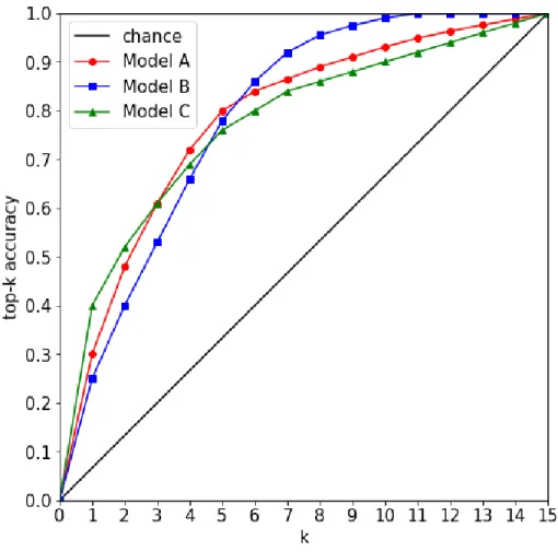
2-3 Example p-ROC curve for a 15-class problem. Three model Top-𝐾 values are plotted (as well as a random chance line that represents an uninformed guesser. . . 35

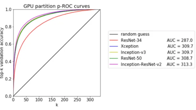
3-1 p-ROC curves for GPU-partition trained models. See Appendix A Figure A-1 for p-ROC in the other training configurations. . . 39

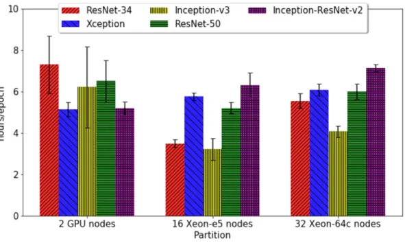
3-2 Training time per epoch on three types of distributed training parti-tions. Error bars indicate standard deviation. . . 40

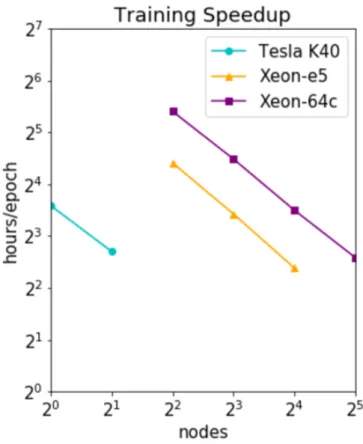
3-3 Training time speedup curve for ResNet-50 backbone model. . . 41

3-4 p-ROC curve log-scaled with 𝑘/339 subtracted out for each value of 𝑘 to more easily show the peak 𝐽 -statistic. . . 43

3-5 Training Time per Epoch across training configurations of 1, 2, 4, 8, 16, and 32 nodes where each node as 2 Volta V100 GPUs. . . 44

3-6 Plotting training time per epoch (in seconds) against p-ROC 𝐴𝑈 𝐶𝑛𝑜𝑟𝑚

to show accuracy-computational performance trade-offs The best per-forming models are in the bottom right: Inception-ResNet-v2, ResNet50, MobileNet-v2, Xception, and DenseNet201. . . 45

4-1 Video ”cubes” are comprised of densely stacked frames. ”Slices” can be taken (1) frame-wise by selecting a particular frame, (2) horizontally by selecting a particular row of pixels across all frames, or (3) vertically by selecting a particular column of pixels across all frames. . . 48

4-2 Examples of slice sampling techniques that can be applied along any axis (slicing method) of the video cube. The left shows uniformly sampling across the axis while the right shows preferentially sampling

4-3 Video slices are first passed through an ImageNet-pretrained VGG Fea-ture Extractor which creates embedded feaFea-ture vectors used as inputs to a three layer network consisting of two 4096-unit fully connected layers followed by a 10-unit fully connected layer that outputs softmax predictions. The second version of the model includes two dropout (𝑝 = 0.5) layers in between the fully connected layers. . . 50

4-4 Visualization of sampling distributions tested in this study. Here, they are centered on 112 which is the center row/column on the video cube when sliced horizontally or vertically. . . 51

4-5 p-ROC validation curves for slicing and sampling on the best perform-ing architecture. With the frame slicperform-ing method, there was little to no difference between sampling techniques. Horizontal slicing method shows the most significant difference between sampling techniques. . . 52

4-6 Average training time per epoch (in minutes) for each slicing method and sampling technique. Error bars indicate standard deviation across epochs. Training times shown are using 2 NVIDIA Volta V100 GPUs with PCIe connection. . . 54

5-1 The top diagram shows an example audio waveform with a sample rate of 22050. The bottom diagram shows the transformation to a Mel-Frequency Spectrogram with a log power scale, 128 mels, and a maximum frequency of 8192 Hz. . . 56

5-2 Process of stitching early audio-video fusion between an RGB frame and the log-mel spectrogram. The input to the ConvNet is a wider 3-channel image. . . 58

5-3 Process of stacking early audio-video fusion between an RGB frame and the log-mel spectrogram. The input to the ConvNet is a 4-channel image with the same pixel height and width as the original frame. . . 59

5-4 p-ROC curve for best and worst performing models using no fusion, stitching fusion, and stacking fusion. "Best" and "Worst" in this figure are referring only to the highest and lowest p-ROC 𝐴𝑈 𝐶 values. . . . 60

5-5 10-Class Fusion Experiment Computational Performance Results when training on 8 NVIDIA Volta 100 GPUs. Note that training time per epoch is plotted on a log scale as horizontal and vertical slicing took significantly longer than frame slicing. Results with Gaussian (𝜎 = 30) sampling are analogous and the plot can be found in Appendix B, Table B-1. . . 61

5-6 The Cross-v1 model architecture that utilizes vertical and horizontal video slices. . . 63

5-7 The Cross-v2 model architecture that utilizes frame, vertical, and hor-izontal video slices. . . 63

5-8 339-class experiment stitching fusion validation results. The colored markers, as labeled in the legend to the right, indicate the various stitching early fusion models. Grayed-out models dots respond to the non-fusion baselines described in Chapter 3. . . 64

5-9 339-class experiment stacking fusion validation results. The colored markers, as labeled in the legend to the right, indicate the various stitching early fusion models. Grayed-out models dots respond to the non-fusion baselines described in Chapter 3. . . 65

5-10 A comparison of stitching early fusion accuracy and computational performance when trained on 64 Volta V100 GPUs (2 per node). The colored markers, as labeled in the legend to the right, indicate the various stitching early fusion models. Grayed-out models dots respond

5-11 A comparison of stacking early fusion accuracy and computational per-formance when trained on 64 Volta V100 GPUs (2 per node). The col-ored markers, as labeled in the legend to the right, indicate the various stitching early fusion models. Grayed-out models dots respond to the non-fusion baselines described in Chapter 3. . . 66

A-1 p-ROC curves for CPU partitions trained models. . . 73

B-1 10-Class Fusion Experiment Computational Performance Results (with Gaussian 𝜎 = 30 sampling). Note that training time per epoch is plotted on a log scale as horizontal and vertical slicing took significantly longer than frame slicing. . . 83

List of Tables

1.1 MIT Supercloud TX-E1/GAIA Specifications (2019–spring 2020). [59] 21

2.1 A Brief History of Neural Network Architectures. . . 28

2.2 Moments in Time Challenge 2018 top-performing single model valida-tion accuracies as described in opvalida-tional report submissions by compe-tition teams. . . 31

2.3 Moments in Time Challenge 2018 top-performing teams approaches as described in optional report submissions by competition teams. . . 32

2.4 p-ROC curve statistics for the 15-class problem plotted in Figure 2-3. 34 3.1 Complexity of "Off-the-Shelf" C2D Model Backbones . . . 38

3.2 Complexity of Models in Expanded Comparison Study . . . 42

A.1 2D Model Comparison of Accuracy Performance. . . 74

A.2 Expanded Comparison - Accuracy Performance . . . 75

A.3 Exploration of Video Slicing and Sampling: validation results each slicing method (frame, horizontal, and vertical). . . 76

A.4 10-Class Early Fusion Study Validation Results. . . 77

A.5 339-Class Early Fusion Study Validation Results. . . 78

B.1 Video and audio parsing computational performance per class (minutes). 79 B.2 2D Model Comparison of Computational Performance. . . 80

B.3 Expanded Comparison - Computational Performance . . . 81 B.4 Exploration of Video Slicing and Sampling: computational

B.5 10-Class Early Fusion Study Computational Performance Results. . . 84

B.6 339-Class Early Fusion Study Computational Performance Results (when trained on 64 Volta V100 GPUs, 2 per node). Note that the last five models in each category are trained as simple C2Ds but then used as 6-frame TSN models for validation video-level inference as described in Chapter 5. Those models were trained for 65 epochs rather than 50 for the other models which is why their total training times are generally higher. . . 85

C.1 Moments in Time Dataset Statistics (at time of download). . . 87

C.2 Overview of Video Action Recognition Datasets. . . 88

Chapter 1

Introduction

Over the last decade, advances in computing hardware and data availability have yielded significant progress in machine learning and artificial intelligence [20]. For ex-ample, applications such as object recognition in images have essentially reached, and in some cases surpassed, the accuracy of human object recognition (e.g., 29 of 38 teams in the 2017 ImageNet [15] Challenge achieving error rates <5%) [23]. However, other applications such as the classification of actions in trimmed and untrimmed videos remain a challenge due to the volume and complexity of analyzing video streams. This project dived into the trimmed action recognition problem with two goals:

1. Presenting a comparison of existing approaches. 2. Testing novel early fusion methods.

Both aspects of the project were enabled by high performance computing (HPC) resources and the availability of curated action recognition datasets.

1.1

Video Action Recognition

Action (or activity) recognition is the computer vision task of identifying what is occurring in a video. Figure 1-1 displays several examples of video frames with their corresponding action (verb) labels. An action recognition model takes a video as an input and produces softmax probability predictions for the action class labels.

Figure 1-1: Example action recognition categories and video screenshots from the Moments in Time dataset [54].

Early approaches to action recognition utilized Hidden Markov Models (HMM) [92] and Dynamic Bayesian Networks (DBN) [91]. Later, Support Vector Machines (SVM) [77] used visual bag-of-words with many hand-crafted spatial, temporal, and spatio-temporal features: Histogram of Oriented Gradient (HOG), HOG3D [41], Histogram of Optical Flow (HOF) [10], Motion Boundary Histogram (MBH) [14], Speeded-Up Robust Features (SURF) [5], KLT Trajectories [51], SIFT Trajecto-ries [71], Dense TrajectoTrajecto-ries (DT) [79], and Improved Dense TrajectoTrajecto-ries (iDT) [80]. However, since approximately 2014, Deep Neural Network (DNN) approaches have eclipsed these traditional methods and yielded better accuracy results on a variety of datasets. DNNs benefit from learning appropriate feature representations from raw data rather than requiring carefully hand-crafted inputs. The successes of deep learning in other computer vision problems such as image recognition, object detec-tion, and scene segmentadetec-tion, beg the question: can DNNs (and Deep Convolutional Neural Networks in particular) follow a similar path with video?

In order to test action recognition approaches, large video datasets have been collected, organized, and labeled. One such dataset is Moments in Time, a

collec-Moments in Time dataset creators in collaboration with CVPR 2018 released the Moments in Time Challenge which encouraged teams to develop models that yield high Top-1 and Top-5 accuracies on the dataset. The top performing team produced an ensemble model with a Top-1 accuracy of 38.64% and a Top-5 accuracy of 67.19%. Clearly, there is significant room for improvement remaining in video action recog-nition, particularly with the classification problem posed by the Moments in Time dataset.

1.2

Modality Fusion

Action recognition is inherently a multi-modal problem with spatial, temporal, and often auditory domain components. The spatial domain is commonly captured in a visual Red-Green-Blue (RGB) modality. The temporal domain is commonly dealt with relationing between spatial data or via video transformations such as to opti-cal flow. Auditory domain information can be encoded in a raw (1D) form or via transformations such as into a (2D) spectrogram.

DNN approaches to learning with multi-modal features can be generally catego-rized as "early fusion" or "late fusion." In early fusion, multi-modal features are fused prior to learning as shown in Figure 1-2. In late fusion, individual mode features are learned in separate networks and then fused via an ensemble learner as shown in Figure 1-3. Early fusion requires only a single session of learning while late fusion requires two (one session for the individual mode features and one to ensemble).

In the video action recognition literature, essentially all best-performing current models use late fusion rather than early fusion for several reasons. First, late fusion benefits significantly from research and testing already completed on the individual modality networks which can be pretrained on similar datasets. For example, a spatial model which trains on video frames can be pretrained on images from ImageNet [15]. Similarly, an audio model which trains on the video’s audio channels can be pretrained on audio clips from AudioSet [22]. Pretraining can help these models generalize beyond an individual dataset’s training data and can speed up training.

Figure 1-2: Generic early fusion architecture (adapted from [68]). Multi-modal fea-tures are extracted and fused prior to being used as input to a supervised learner.

Figure 1-3: Generic late fusion architecture (adapted from [68]). Multi-modal features are extracted and fed as inputs to separate supervised learned. The outputs of those learners are fused and fed as inputs to another supervised learner which typically consists of only a few dense layers to do classification and end with softmax output.

Second, data parsing, wrangling, and fusing necessary for early feature fusion on large datasets is computationally costly. Without sufficient computational resources for these data augmentation steps (often in the form of a distributed computing system) or money to access one (such as Amazon Web Services), late fusion is more appealing as it can often be done on smaller systems.

Third, it can be argued that late fusion research is more tried and true. With early fusion, researchers must often take a "gamble" when designing new multi-modal

Table 1.1: MIT Supercloud TX-E1/GAIA Specifications (2019–spring 2020). [59] Intel Xeon Intel Xeon AMD Intel Xeon Intel Xeon

E5-2650 E5-2683 Opteron E5-2680 G6-6248 Number of nodes 25 7 20 4 224

CPU cores/node 16 2 x 14 2 x 16 2 x 14 2 x 20

GPUs/node 0 0 0 2 or 4 2

GPU type N/A N/A N/A Volta V100 Volta V100

RAM (GB) 64 256 192 500 384

Local Disk (TB) 16 12 8 2 3.8

methods. Experimentation can be the only way of truly determining the effectiveness of an early fusion approach. Meanwhile late fusion can take the best existing model or models for each individual modality. Therefore, late fusing well-studied single-modality models is the default that most action recognition research uses and this is reflected in the Moments in Time Challenge 2018 results.

1.3

High Performance Computing

High performance computing (HPC) refers to employing aggregated computing power to achieve performance not possible through normal workstation computing. HPC was critical in this project because of the computational demands of working with videos. Video data, consisting of dozens of frames and additional audio channels, is orders of magnitude more data dense than image data. For example, ImageNet is approximately 150 GB of raw data [65] while Moments in Time is 42 TB of data after cropping to 224x224 frame size and parsing into NumPy [56] arrays.

Throughout this project, the HPC resources of GREEN, E1, and TX-GAIA (Supercloud) via MIT Lincoln Laboratory were instrumental in speeding up all aspects of the parse-wrangle-train-analyze pipeline. Parsing and wrangling were easily parallelized by action class via a mapping function. Training and validation were parallelized across compute nodes and/or GPUs via OpenMPI and Horovod [63]. An overview of the MIT Supercloud (TX-E1) infrastructure is provided in Table 1.1 and a detailed description can be found in [59].

Figure 1-4: Overview of the Training Pipeline.

1.4

Training Pipeline

The first phase of this project involved constructing a pipeline for working with video data on the HPC systems described in section 1.3. Figure 1-4 describes the steps in that parse-wrangle-train-analyze pipeline. Some prior, yet incomplete work had been done on FFmpeg extraction of raw video frames by a previous LLSC intern, but the bulk of the pipeline was created during this project.

Moments in Time dataset raw video frames (stored in .mp4, .gif, and other com-mon video file formats) were extracted at 30 frames per second (fps) using FFM-PEG and converted into three-channel (RGB) 224x224x3 pixel tensors and stored as NumPy [56] arrays in HDF5 files (one per action class). Audio was parsed at both sample rates of 37.9KHz and 15.2KHz, transformed into log-mel spectrograms with 224 mels and a max frequency of 8192 Hz, and saved as one-channel images. Further audio parsing details can be found in section 5.1. Runtime statistics for parsing and transforming the training and validation data can be found in Appendix B, Table B.1. If those operations were performed serially on an Intel Xeon-e5 core, parsing the

the job across 60 cores using MIT Supercloud HPC resources.

An optional wrangling stage occured when only particular aspects of the data are required. This includes additional pre-processing (see Chapter 4 for examples). Parsed/wrangled videos were then fed into a model which outputs softmax predictions across the class options. Models were trained on a training set and evaluated on a validation set.

1.5

Project Overview

At a high level, this project had two goals. The first was to present a comparison of computational performance and accuracy of existing models using the Moments in Time training and validation sets. The second was to attempt to approach or surpass current performance and/or accuracy using novel features and architectures. The project therefore involved (1) constructing a training pipeline for using the Moments in Time dataset, (2) exploring feature engineering with early fusion of video and audio modalities, (3) investigating video action recognition architectures and hyperparam-eter selection, and (4) applying high performance computing methods to engineered features and models.

Chapter 2 presents a background on action recognition datasets and machine learning approaches. It also highlights research decisions made when designing these studies including why 2D models are the centerpiece of this research and how the action recognition approaches will be evaluated. Chapter 3 describes the compari-son study implemented and conducted to baseline accuracy performance and com-putational performance of some action recognition models. Chapter 4 describes the slicing and sampling study implemented and conducted to investigate 2D spatial and spatio-temporal features. Chapter 5 describes the early fusion study implemented and conducted to investigate audio-video fusion using results obtained from the com-parison study and the slicing and sampling study. Chapter 6 presents conclusions from this project, both from the literature review and the experiments, as well as recommendations for avenues to continue and expand upon this research.

Chapter 2

Background, Related Work, and

Model Assessment

This chapter presents a background on video datasets and machine learning ap-proaches to the action recognition problem. It will then explain why the Moments in Time dataset is used throughout these experiments and what model assessment techniques are appropriate for adequately comparing accuracy performance and com-putational performance.

2.1

Action Recognition Datasets

Datasets for video action recognition are defined by a set of qualities: source, pre-processing, point-of-view, number of videos, length of each video, number of action classes, classes per video (single-label or multi-label), annotation style, and purpose. A myriad of datasets have been crafted and curated to span this spectrum of qualities. The vast majority of these video datasets focus exclusively on human actions for the obvious reason that human actions are extremely relevant to all aspects of everyday life. Early datasets, KTH [62], Weizmann [6], GTEA [18], GTEA GAZE [17], and GTEA GAZE+ [17], were created by research groups focused on daily human activities. Spurred by the growth of online video, UCF101 [69] and HMDB51 [44], with 13,000 and 7,000 videos, respectively, quickly became foundational benchmarks

Figure 2-1: Action Recognition Dataset Zoo. Two screenshots are taken from separate videos in each of the labeled datasets, giving a glimpse into the quality and focus of each of each.

in human action recognition. Thumos [36] and ActivityNet [29] had similar goals but did not gain the same level of popularity in the literature.

While human actions and human activities continue to dominate the field of action recognition datasets, slowly other purposes of these datasets emerged. Among them, YouTube-8M [2] and Micro-Videos (MV) [55] focused on human and non-human actions and visual entities. The Something-Something [24] dataset looks at low-level action captions for intuitive physics and semantics.

Among the most current iterations of these datasets, only a few have the breadth (action classes) and depth (videos per action class) that are comparable to ImageNet and other object recognition datasets. Kinetics-600 [8] and VLOG [19] achieve this for human actions and daily interactions. Moments in Time [54], which will be described in further detail in section 2.3, also achieves this quality. For a more detailed timeline of the creation of these datasets as well of information about dataset size and number of classes, see Appendix C, Table C.2.

2.2

Machine Learning for Action Recognition

Deep CNNs for computer vision proved their worth in 2012 with the application of AlexNet [43] to the ImageNet Large-Scale Visual Recognition Challenge (ILSVRC). Table 2.2 provides a timeline of major CNN architecture breakthroughs in computer vision specifically emphasizing those useful in common action recognition approaches. With these developments, action recognition model architectures can be broadly cat-egorized into two groups: 2D approaches and 3D approaches.

2D action recognition models are categorized as 2D not because they ignore the temporal domain aspect, but because they use 2-Dimensional convolutional kernels generally in the form of 2D CNN model backbones. These approaches include tradi-tional 2D Convolutradi-tional Neural Networks (C2D), Temporal Segment Networks (TSN) [87], Long-term Recurrent Convolutional Neural Networks (LRCN) [16] sometimes referred to as CNN+LSTMs, and Temporal Shift Modules (TSM) [49]. C2D carries over directly from image recognition. A frame is extracted from the video and used

Table 2.1: A Brief History of Neural Network Architectures.

Accuracy (%)

Architecture Year Description UCF HMDB Kinetics LeNet [45] 1998 pioneered CNNs

AlexNet [43] 2012 introduced ReLU & max pool VGG [67] 2014 deeper net with smaller kernels Inception [74, 75] 2014 inception cell convolves at

(GoogLeNet) multiple scales then aggregates

2-Stream CNN [66] 2014 late fusion of a spatial and 88.0 59.4 optical-flow based temporal nets

ResNet [28, 89] 2015 residual block learns a

residual function of the input

C3D [76] 2015 extended 2D convolution to 3D 90.4 𝐹𝑆𝑇𝐶𝑁 [72] 2015 factorized 3D kernel as 2D 88.1 59.1

spatial followed by 1D temporal

TDD [81] 2015 combined hand-crafted & deep- 91.5 65.9 learned features

CNN+LSTM [16] 2015 CNN followed by an LSTM for 82.7 (LRCN) sequence-based actions

SqueezeNet [31] 2016 decreased parameter-space with AlexNet-level results

TSN [87] 2016 learns temporal structure via 94.2 69.4 segment/two-stream/consensus

ResNeXt [86] 2017 replaced residual blocks with a “split-transform-merge” block Xception [12] 2017 improved inception cell by

performing 1x1 convolution first then channel-wise spatial

Two-Stream I3D [9] 2017 two-3D convolutional streams 97.9 80.2 on dense RGB and optical flow

DenseNet [32] 2017 connected every layer to every successive network layer SENet [31] 2018 modified residual block for

channel interdependencies

NL [82] 2018 introduced a non-local block for 77.7 long dependencies

TRN [93] 2018 used a temporal relations pool 83.8 63.2 instead of TSN’s average pool

MKAF [50] 2018 multi-modal keyless attention 77.0 fusion for fast LSTM

Figure 2-2: Four most common video action recognition approaches. Note that these are simplified diagrams where icons for 2D-ConvNets, 3D-ConvNets, dense classifica-tion networks, LSTM modules, and averaging/softmax layers are used only as visual interpretation. Their actual design can vary significantly. Similarly, the majority of action recognition approaches have 2-stream variants for RGB+Optical Flow.

as input to a 2D-ConvNet. After several convolution and pooling layers, the logits are fed into one or more fully-connected layers which can produce a softmax output predictions over the classes. TSN segments a video along its temporal dimension and extracts a frame from each segment. The frames are used as inputs to a 2D-ConvNets that share weights. The predictions from each segment are then averaged before the softmax output. Variants and additions to a TSN baseline include Temporal Rela-tions Networks (TRN) [93] which perform multi-scale segmentation and relationing. LRCN similarly segments a video, extracts a frame from each segment and feeds those frames into 2D-ConvNets. However, the ConvNet outputs are used as inputs to a Long-Short Term Memory (LSTM) network. The LSTM’s output is used for softmax predictions.

3D action recognition approaches include the temporal aspect in the convolution via the use of 3-Dimensional convolutional kernels. C3D models were designed as the 3D analogy to 2D CNNs because of the widespread success of 2D CNNs [76]. However, because of the difficulties of working with videos and the long-term dependencies aspects of actions, C3D models often have had less success on action recognition than

their 2D counterparts on object recognition. To attempt to bridge the gap between 2D and 3D models, Inflated 3D (I3D) models were created by ”inflating” pretrained 2D kernels into 3D kernels [9]. This allows I3D models to benefit from pretraining on 2D image datasets like ImageNet. Some believe that, while still in their early days, 3D approaches will be able to retrace the successful history of their 2D siblings [27]. Both C3D and I3D work by using either the entire or a selected portion (often 16, 32, or 64 frames) as an input to a 3D-ConvNet. Similar to C2D, the 3D-ConvNet’s output is then fed into a one or more layer classification network before outputting softmax predictions across classes.

2.3

Moments in Time

Among action recognition datasets, Moments in Time uniquely offers high inter-class and intra-inter-class variation [54]. Inter-inter-class variation refers to a large semantic separation between the 339 action verb classes. Intra-class variation refers to various levels of abstraction within each action verb class. For example, the "opening" class can include videos of opening doors, drawers, curtains, flower petals, and more. The actions can be performed by various agents: humans, animals, animations, or nature. Each 3-second video in the dataset has a single action verb label from one of the 339 action classes. The training set consists of 802,264 videos with between 500 and 5,000 videos per class. The validation set consists of 33,900 videos with 100 videos per class. High-level dataset statistics can be found in Appendix C, Table C.1.

The Moments in Time dataset creators tested a variety of existing action recogni-tion model architectures on their dataset (see Appendix C, Table C.3) as well as ran two challenges as a part of CVPR’18 and ICCV’19. The 2018 challenge tasked teams to develop state-of-the-art methods for achieving top-1 and top-5 accuracies on the dataset. Essentially all top-performing teams used late fusion approaches by training a series of individual models and then ensembling their results. Table 2.2 highlights the best-performing individual models used by teams in the challenge as described in

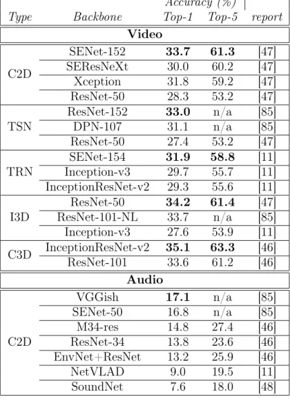
Table 2.2: Moments in Time Challenge 2018 top-performing single model validation accuracies as described in optional report submissions by competition teams.

Accuracy (%)

Type Backbone Top-1 Top-5 report Video C2D SENet-152 33.7 61.3 [47] SEResNeXt 30.0 60.2 [47] Xception 31.8 59.2 [47] ResNet-50 28.3 53.2 [47] TSN ResNet-152 33.0 n/a [85] DPN-107 31.1 n/a [85] ResNet-50 27.4 53.2 [47] TRN SENet-154 31.9 58.8 [11] Inception-v3 29.7 55.7 [11] InceptionResNet-v2 29.3 55.6 [11] I3D ResNet-50 34.2 61.4 [47] ResNet-101-NL 33.7 n/a [85] Inception-v3 27.6 53.9 [11] C3D InceptionResNet-v2 35.1 63.3 [46] ResNet-101 33.6 61.2 [46] Audio C2D VGGish 17.1 n/a [85] SENet-50 16.8 n/a [85] M34-res 14.8 27.4 [46] ResNet-34 13.8 23.6 [46] EnvNet+ResNet 13.2 25.9 [46] NetVLAD 9.0 19.5 [11] SoundNet 7.6 18.0 [48]

of the top-performing teams. While model architectures such as C3D, I3D and TRN may intuitively be expected to provide significant accuracy performance advantages, when applied to the Moments in Time dataset, these architectures barely outperform, and in some cases underperform, conventional and less complex 2D CNN models. Ad-ditionally, while the literature on action recognition lacks an adequate discussion of computational performance and complexity of training these models, it is sometimes hinted that 3D approaches requires significantly more computational resources and time to train.

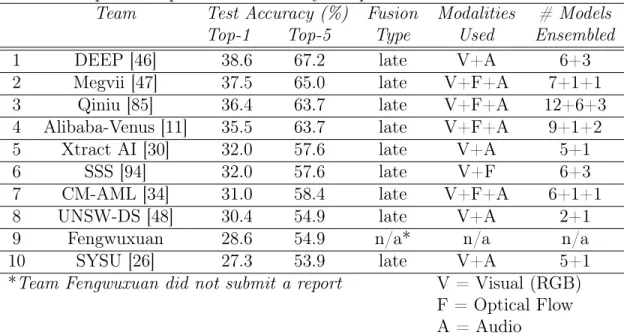
Table 2.3: Moments in Time Challenge 2018 top-performing teams approaches as described in optional report submissions by competition teams.

Team Test Accuracy (%) Fusion Modalities # Models Top-1 Top-5 Type Used Ensembled 1 DEEP [46] 38.6 67.2 late V+A 6+3 2 Megvii [47] 37.5 65.0 late V+F+A 7+1+1 3 Qiniu [85] 36.4 63.7 late V+F+A 12+6+3 4 Alibaba-Venus [11] 35.5 63.7 late V+F+A 9+1+2 5 Xtract AI [30] 32.0 57.6 late V+A 5+1 6 SSS [94] 32.0 57.6 late V+F 6+3 7 CM-AML [34] 31.0 58.4 late V+F+A 6+1+1 8 UNSW-DS [48] 30.4 54.9 late V+A 2+1 9 Fengwuxuan 28.6 54.9 n/a* n/a n/a 10 SYSU [26] 27.3 53.9 late V+A 5+1 *Team Fengwuxuan did not submit a report V = Visual (RGB)

F = Optical Flow A = Audio

teams to develop state-of-the-art methods for detecting multiple event labels from videos. Of the reports that teams submitted, few deviated from 2D CNN approaches likely because they drew the same conclusions as described above in addition to the difficulties that come with working on more complex models. For these reasons, the studies conducted in this project also focus heavily on 2D CNN action recognition methods.

The results of these challenges (demonstrating significant room for improvement), the uniqueness of the dataset, and the potential for 2D approach improvements made Moments in Time the focus of this project.

2.4

Model Assessment Techniques

Video action recognition models are primarily assessed along accuracy performance and secondarily assessed along computational performance. Accuracy performance refers to how effective a trained model is at the action recognition task. Compu-tational performance refers to the compute required to perform the training. Both

between them. A model with high accuracy performance that takes hundreds of years to train is not an effective model. Obviously, neither is a model that trains quickly but has poor accuracy results. Therefore, while often overlooked in the literature, including both aspects of the assessment together is instrumental in comparing video action recognition approaches.

Canonically, Top-𝑘 accuracy is used to measure the effectiveness of action recog-nition models. The model’s softmax output yields a probability for each of the |𝐶| possible classes where 𝐶 is the set of action classes. If the correct class label is within the 𝑘 highest probability predicted classes, the model has successfully classified the video. Top-1 accuracy is intuitively useful because it describes the percentage of vali-dation data cases in which the model’s top predicted classification is correct. However, Top-5 is arbitrarily chosen and has unfortunately become a default in the literature.

This project demonstrates that plotting what will be referred to as a psuedo-Receiver Operator Characteristic (p-ROC) curve is a better method of representing accuracy performance. In this p-ROC, the Top-𝑘 accuracy is plotted against 𝑘 analo-gous to plotting the true positive rate against the false positive rate for our classifier. Even though it has been noted that the ROC area under the curve (𝐴𝑈 𝐶) and the maximum Youden index (𝐽𝑚𝑎𝑥), the curve height about the chance line, provide

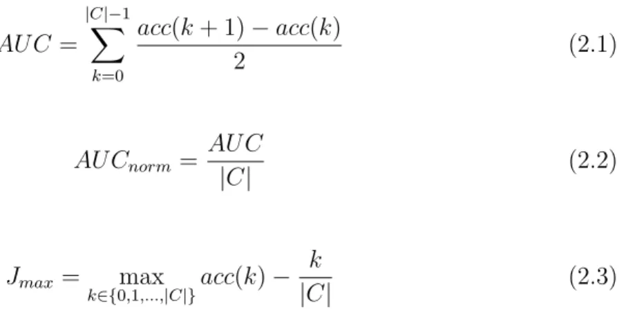
desir-able properties as a classification metric [7, 33], the practice has not become standard. These benefits easily transfer to our p-ROC curve and allow a user to quickly and more intuitively select a model with accuracy characteristics that they desire. One key difference between the p-ROC curve and a traditional ROC curve is that the hor-izontal axis is discrete, not continuous. Hence the Youden index, sometimes referred to as Youden’s 𝐽 -statistic, is only defined at these discrete values of 𝑘. An additional advantage p-ROC 𝐴𝑈 𝐶 is that it can be normalized via dividing by the number of classes |𝐶|. This allows model accuracy comparison across datasets with different numbers of classes (which is common among the datasets mentioned in Section 2.1). Equations 2.1, 2.2, and 2.3 show how to calculate p-ROC 𝐴𝑈 𝐶, 𝐴𝑈 𝐶𝑛𝑜𝑟𝑚, and 𝐽𝑚𝑎𝑥

𝐴𝑈 𝐶 = |𝐶|−1 ∑︁ 𝑘=0 𝑎𝑐𝑐(𝑘 + 1) − 𝑎𝑐𝑐(𝑘) 2 (2.1) 𝐴𝑈 𝐶𝑛𝑜𝑟𝑚 = 𝐴𝑈 𝐶 |𝐶| (2.2) 𝐽𝑚𝑎𝑥= max 𝑘∈{0,1,...,|𝐶|}𝑎𝑐𝑐(𝑘) − 𝑘 |𝐶| (2.3)

The example 15-class classification problem shown in Figure 2-3 is intended to illustrate the usefulness of p-ROC curves in action recognition model accuracy per-formance analysis. Shown in the figure are three models (𝐴, 𝐵, and 𝐶) as well as what would be expected from a random chance guess (i.e. the 𝑘/15 line). Table 2.4 shows summary statistics for comparing these models along traditional Top-1 and Top-5 accuracies as well as with p-ROC 𝐴𝑈 𝐶 and 𝐽𝑚𝑎𝑥. The best-to-worst ordering

of these models along Top-1 accuracy is 𝐶, 𝐴, 𝐵. Along Top-5 accuracy, the order-ing is 𝐴, 𝐵, 𝐶. Therefore, without usorder-ing p-ROC 𝐴𝑈 𝐶, one might naively conclude that Model 𝐵 is worse at this classification task than models 𝐴 and 𝐶. However, Model 𝐵 holds the highest p-ROC 𝐴𝑈 𝐶 among the three models. Clearly, determin-ing the "best" model is no longer straightforward. Because different applications of action recognition problems might require different accuracy performance properties, reporting a p-ROC curve instead of simply the canonical Top-1/Top-5 accuracies is beneficial to the model user. Importantly, we claim that higher Top-5 accuracy does not always correlate with higher p-ROC metrics. This project not only demonstrates that this claim is sometimes true but rather it is fairly common.

Table 2.4: p-ROC curve statistics for the 15-class problem plotted in Figure 2-3. Model Top-1 Accuracy Top-5 Accuracy p-ROC AUC 𝐽𝑚𝑎𝑥

Chance 0.067 0.333 7.50 0.0 𝐴 0.300 0.800 11.72 0.47 (𝑘 = 5) 𝐵 0.250 0.780 11.82 0.46 (𝑘 = 6) 𝐶 0.400 0.760 11.56 0.43 (𝑘 = 5)

Figure 2-3: Example p-ROC curve for a 15-class problem. Three model Top-𝐾 values are plotted (as well as a random chance line that represents an uninformed guesser.

Because of the challenges with dealing with video as opposed to simpler uni-modal classification problems such as image object recognition, computational performance of training is a second important method of assessing models. Unfortunately the lit-erature on action recognition model computational performance is extremely lacking in detail. Almost all emphasis has been place on Top-1/Top-5 accuracy performance. Throughout this project, computational performance is measured directly by train-ing time and traintrain-ing time per epoch. Attention was also paid to how varytrain-ing the compute resources affects training (i.e. yields speedup curves).

Therefore, throughout this project, the accuracy performance and computational performance metrics described above are used to assess models and training tech-niques applied to the Moments in Time dataset.

Chapter 3

Comparison Study

Unlike the field of image classification, video action recognition lacks a thorough dis-cussion of model and algorithm comparison. For example, it is difficult to compare accuracy metrics of various algorithms which are often developed and tested on het-erogenous datasets or lack sufficient details regarding model architectures. Further, the race for higher Top-1 accuracies has sidelined discussions of the equally relevant aspect of computational performance. Therefore, this set of experiments catalogs a subset of state-of-the-art video action recognition models. The goal is to provide a side-by-side comparison of these "off-the-shelf" models using the performance metrics outlined in section 2.4.

Specifically, this study (1) utilized the Moments in Time dataset for action recog-nition model comparison, (2) trained and evaluated a set of action recogrecog-nition models under similar hyperparameters, training methods, and hardware, and (3) discussed both their accuracy performance and computational performance.

3.1

Initial Comparison

A first set of comparisons was between five “off-the-shelf” TensorFlow [1] C2D mod-els: ResNet34 [28], ResNet50 [86], Inception-v3 [74], Inception-ResNet-v2 [73], and Xception [12]. Table 2 shows a comparison of the complexity of these models, and they are listed in increasing order of trainable parameters.

Table 3.1: Complexity of "Off-the-Shelf" C2D Model Backbones Model Layers Trainable Parameters ResNet34 34 21,471,379 Xception 71 21,501,563 Inception-v3 48 22,462,963 ResNet50 50 24,229,203 Inception-ResNet-v2 164 54,797,235

3.1.1

Experimental Design

Python 3.6.5 scripts trained and validated these off-the-shelf models in a distributed fashion using Horovod 0.16.1 [63] and OpenMPI. Key package versions used were NumPy 1.14.1 [56], H5py 2.7.1 [13], SciPy 1.1.0 [78], TensorFlow 1.13.1 [1], PyTorch 1.0.1 [57], Pillow 5.1.0 and FFmpeg 3.3.7.

To compare computational performance and the effects of batch size, three types of distributed training situations were tested. The first used 8 NVIDA Tesla K40 GPU accelerators across two nodes. The second used 16 Intel Xeon-e5 nodes with 28 CPU cores per node. The third used 32 Intel Xeon-64c nodes with 64 cores per node. The infrastructure used is described in detail in [59].

The Moments in Time pre-processed 30 frames per second (fps) videos resized to 224x224 cropped 3-channel frames were used as inputs. Videos were parsed at 15 fps in addition to the 30 fps parsing described in section 1.4. This was completed for training and validation sets that were defined by the Moments in Time creators.

With the exception of ResNet34, which was initialized with random weights, mod-els were initialized with ImageNet pretrained weights. A dense classification layer was added to the top of each of these CNNs. Each network was trained by randomly sampling one frame from each 15 fps parsed video. A Horovod-wrapped distributed stochastic gradient descent (SGD) optimizer and categorical cross-entropy loss metric updated network weights. The learning rate started at 0.1 and decayed by a factor of 10 at 30 epochs. It was also adjusted during the first 5 (warmup) epochs, increased by a factor of the total number of processes launched. Standard momentum of 0.5

Figure 3-1: p-ROC curves for GPU-partition trained models. See Appendix A Figure A-1 for p-ROC in the other training configurations.

For proper comparison, other hyperparameters were held consistent across differ-ent model training sessions. Each model was trained for 50 epochs with a batch size of 32 per training process. One process was launched per Tesla K40 GPU yielding an effective batch size of 256 on the GPU nodes partition. On each of the CPU node partitions, one process was launched per node yielding effective batch sizes of 512 and 1024 on Xeon-e5 node partitions and a Xeon-64c node partitions, respectively.

Trained C2Ds were expanded into TSNs for validation inference. Video level inference was therefore the averaged prediction across 6 evenly spaced frames from the 90 frame (30 fps) video.

3.1.2

Accuracy Performance Results

After 50 epochs, models with pretraining averaged 22.1% 1 and 45.7% Top-5 accuracy using the smallest effective batch size corresponding to the GPU nodes partition. The ResNet34 model that did not benefit from pretraining performed worse. The Inception-ResNet-v2 model, which has significantly higher complexity than the

Figure 3-2: Training time per epoch on three types of distributed training partitions. Error bars indicate standard deviation.

other models, had the greatest Top-1 accuracy, Top-5 accuracy, p-ROC 𝐴𝑈 𝐶, and 𝐽𝑚𝑎𝑥. The p-ROC curves are shown in Figure 3-1 and full validation results are shown

in Appendix A Table A.1.

3.1.3

Computational Performance Results

The computational performance of models averaged around 6 hours per epoch on a 2-node GPU partition, 5 hours per epoch on a 16-node Xeon-e5 partition, and 6 hours per epoch on a 32 node Xeon-64c partition. On GPU nodes, model training time fluctuated between 4 and 9 hours per epoch and saw higher variation than models trained on Xeon-e5 or Xeon-64c nodes. As shown in Figure 3-2, the best performing model in accuracy (with an Inception-ResNet-v2 backbone) had similar computational costs to other models across partition types despite having twice as many parameters and two to three times as many layers.

Figure 3-3: Training time speedup curve for ResNet-50 backbone model.

the standard deviation of training time per epoch varied by no more than 1.5 hours. These results further show, as has been noted in the literature [38], that the number of floating-point operations does not always directly correspond to computational costs due to other training time activities. Further research is needed to identify which aspects of training are contributing the most to the computational performance costs. However, these results are still a valuable start to researchers working with C2D models for action recognition who may not initially know what computational resources and time are required for training models. This is particularly relevant because of the monetary costs involved in using cloud-based resources like AWS.

Figure 3-3 shows the speedup curve for training a ResNet50 model. Other C2D models should have analogous speedup curves. Across the three partitions, a 2x increase in nodes directly yielded a 2x reduction in training time.

Table 3.2: Complexity of Models in Expanded Comparison Study Model Type Model Backbone Layers Trainable Parameters

C2D VGG19 19 20,198,291 MobileNet (M) 28 3,554,451 Inception-v3 (Iv3) 48 22,462,963 ResNet50 (R50) 50 24,229,203 MobileNet-v2 (Mv2) 53 2,658,131 Xception (X) 71 21,501,563 Inception-ResNet-v2 (IRv2) 164 54,797,235 DenseNet169 (D169) 169 13,048,915 DenseNet201 (D201) 201 18,744,147 LRCN n/a (16f) 38 9,788,915 C3D n/a (16f) 18 148,590,675 n/a (32f) 18 456,872,019 I3D Inception-v1 (Iv1) (16f) 27 12,279,984

Inception-v1 (Iv1) (64f) 27 12,279,984

3.2

Expanded Comparison

Due to increased computational resource availability later in this research, the com-parison study was able to be expanded to include more TensorFlow action recognition models and greater breath of computational performance testing. Table 3.2 lists de-tails of the models compared.

3.2.1

Experimental Design

Python 3.6.5 scripts trained and validated these off-the-shelf models in a distributed fashion using Horovod 0.18.2 [63] and OpenMPI 4.0. Key package versions used were NumPy 1.16.5 [56], H5py 2.9.0 [13], SciPy 1.3.2 [78], and TensorFlow 1.14.0 [1].

C2D and I3D models were initialized with ImageNet pretrained weights while C3D and LRCN models were initialized with random weights. On each pass through the dataset during training, C2D inputs were randomly sampled frames from each video. LRCN, C3D (f16), and I3D (f16) had inputs of 16 evenly spaced frames from the 30 fps videos. C3D (32f) and I3D (64f) randomly sampled 32 and 64 continuous frames,

Figure 3-4: p-ROC curve log-scaled with 𝑘/339 subtracted out for each value of 𝑘 to more easily show the peak 𝐽 -statistic.

For proper comparison, other hyperparameters were held consistent across dif-ferent model training sessions. A Horovod-wrapped distributed ADADELTA [90] optimizer and categorical cross-entropy loss metric updated network weights. Five warmup epochs slowly raised the learning rate to 1.0 which was subsequently decayed at 20, 35, and 50 epochs. Each model was trained for 65 epochs.

For validation, LRCN, C3D, and I3D model inference was performing the same as training. C2D model inference was performed in a TSN-style averaging across 6 evenly spaced frames for the 90 frame (30 fps) video.

3.2.2

Accuracy Performance Results

Validation accuracy results can be found in Figure 3-4 and in detail in Appendix A, Table A.2. By our p-ROC, the top three performing models were all C2Ds:

Inception-Figure 3-5: Training Time per Epoch across training configurations of 1, 2, 4, 8, 16, and 32 nodes where each node as 2 Volta V100 GPUs.

ResNet-v2, DenseNet169, and Xception with p-ROC 𝐴𝑈 𝐶s of 310.99, 310.32, and 310.02, respectively.

3.2.3

Computational Performance Results

Computational performance results can be found in Figure 3-5 and in detail in Ap-pendix B, Table B.3. As expected, LRCN, C3D, and I3D models had significantly greater training times compared to the much simpler C2D models. When training on 64 GPUs for 65 epochs, the quickest model was ResNet50 which had an average training time of 335.4 seconds per epoch. Therefore, the model successfully trained in just over six hours.

Figure 3-6: Plotting training time per epoch (in seconds) against p-ROC 𝐴𝑈 𝐶𝑛𝑜𝑟𝑚

to show accuracy-computational performance trade-offs The best performing models are in the bottom right: Inception-ResNet-v2, ResNet50, MobileNet-v2, Xception, and DenseNet201.

tions on the TX-GAIA system became more apparent in the larger (16 and 32 node) training runs as evidenced by the increased variation on the right of Figure 3-5.

3.3

Discussion and Conclusions

Two comparison experiments comprised this study. The first looked at five off-the-shelf C2D models trained in both GPU and CPU environments. The second expanded the number of C2D models analyzed and incorporated more complex LRCN, C3D, and I3D models. When combining accuracy and computational performance into a single plot, as shown in Figure 3-6, the best performing models are in the bottom right. Those correspond to high p-ROC 𝐴𝑈 𝐶𝑛𝑜𝑟𝑚 and low trainings times per epoch.

Among the models tested, it is apparent that C2Ds are better performers than their more complex counterparts. Among the C2Ds, those with greatest model depth stand out. This hints that deeper is the direction to go with future model architecture research.

Chapter 4

Exploration of Video Slicing and

Sampling

The use of 2D convolutional kernels in video action recognition models remains widespread, yet the literature shows a functional fixedness on using frame-wise train-ing methods. This study explored horizontal and vertical video cube slictrain-ing methods as well as several sampling techniques for determining where along a given video axis to "slice." In this study, frame slicing refers to extracting a frame (𝑝𝑖𝑥𝑒𝑙𝑠 x 𝑝𝑖𝑥𝑒𝑙𝑠 x 𝑐ℎ𝑎𝑛𝑛𝑒𝑙𝑠) from a video (𝑓 𝑟𝑎𝑚𝑒𝑠 x 𝑝𝑖𝑥𝑒𝑙𝑠 x 𝑝𝑖𝑥𝑒𝑙𝑠 x 𝑐ℎ𝑎𝑛𝑛𝑒𝑙𝑠) and then training the 2D kernel on that frame. The frame is a spatial representation for a portion of that video. Horizontal and vertical slicing methods extract a spatio-temporal feature from a video. Essentially, by taking a particular row or column of pixels across the entire temporal domain (i.e. that row/column in every frame), a spatio-temporal ”image” is extracted from the video "cube" with a shape (𝑓 𝑟𝑎𝑚𝑒𝑠 x 𝑝𝑖𝑥𝑒𝑙𝑠 x 𝑐ℎ𝑎𝑛𝑛𝑒𝑙𝑠). The video cube slicing methods are shown in Figure 4-1. Within each slicing method, it is also possible to vary the sampling technique—how to select a given row/column/frame from those available. Figure 4-2 shows example sampling techniques along a slicing axis. One might presume that the center of the video is more likely to include the action occurring. When a camera operator films an action, it is likely that they are centering the action in the shot rather than intentionally keeping it on the edge of the frame (especially in internet-sourced low-quality videos such as those found in the

Figure 4-1: Video ”cubes” are comprised of densely stacked frames. ”Slices” can be taken (1) frame-wise by selecting a particular frame, (2) horizontally by selecting a particular row of pixels across all frames, or (3) vertically by selecting a particular column of pixels across all frames.

Moments in Time dataset).

Specifically, this study (1) compared horizontal and vertical cube slicing methods to the traditional frame-wise slicing in 2D CNN action recognition models and (2) compared six sampling techniques for determining where to slice the cube in each of the methods.

4.1

Experimental Design

Training was conducted using 2 NVIDIA Volta 100 GPU accelerators on a single compute node connected by PCIe. The node uses 2x14 Intel Xeon E5-2690v4 CPU cores with 512 GB of RAM and 2 TB of local disk storage. Each validation run was conducted on a single compute node using 2x16 AMD Opteron CPU cores with a total of 128 GB of RAM and 8TB of local disk storage. Scripts were written in Python 3.6.5 and distributed training used Horovod 0.16.1 [63]. Key package versions used were NumPy 1.14.3 [56], H5Py 2.7.1 [13], SciPy 1.1.0 [78], TensorFlow 1.13.1 [1], and Pillow 5.1.0.

Figure 4-2: Examples of slice sampling techniques that can be applied along any axis (slicing method) of the video cube. The left shows uniformly sampling across the axis while the right shows preferentially sampling the center of the axis using a Gaussian distribution.

classes (applauding, baking, crashing, descending, eating, flooding, guarding, hitting, inflating, jumping) of the 339 in the dataset were used. Therefore, this project made the simplifying assumption that the results obtained from these slicing and sampling comparisons will correlate with performances attained on the entire dataset. This assumption is reasonable because of the high interclass variance in the Moments in Time dataset [54]. Given this simplification, the training set includes 27,494 videos and the validation set includes 1,000 videos. In their parsed form, the videos from these 10 classes are over 1.4 Terabytes of data.

A feature embedding for each video frame slice, horizontal slice, and vertical slice was created by passing each slice through an ImageNet pretrained VGG networks with the top dense layers removed. This results in a (1 x 7068) vector for each horizontal or vertical slice and a (1 x 25088) vector for each frame.

Two model architectures were used. The first was the standard VGG-top layers (two 4096 unit fully-connected layers followed by a 10 unit fully connected layer with softmax output). The second was the same VGG but with two dropout layers inserted (𝑝 = 0.5) after each 4096 unit fully-connected layer. Both models were initialized with random weights. This model is displayed in Figure 4-3.

For each model and slicing technique, the network was trained by sampling a slice from the video. Six sampling techniques were tried for each model and slicing

Figure 4-3: Video slices are first passed through an ImageNet-pretrained VGG Feature Extractor which creates embedded feature vectors used as inputs to a three layer network consisting of two 4096-unit fully connected layers followed by a 10-unit fully connected layer that outputs softmax predictions. The second version of the model includes two dropout (𝑝 = 0.5) layers in between the fully connected layers.

method. Slices were sampled at random from either a Uniform distribution over the pixels rows/cols or frames (depending on slicing method) or from a Gaussian distribution centered on the center-row/col or center frame with a standard deviation (𝜎) of 5, 10, 20, 30, or 40. These distributions when applied to horizontal/vertical slicing are shown in Figure 4-4.

A Horovod wrapped distributed stochastic gradient descent (SGD) optimizer and categorical cross-entropy loss metric update the network weights. The learning rate starts at 0.01 and is decayed by a factor of 10 at 30 epochs. It is also adjusted during the first five (warmup) epochs with respect to the number of processes launches. Stan-dard momentum of 0.5 is used. Each model is trained for 50 epochs (or for 12 hours, whichever occurs first) with a batch size of 32 per process yielded an effective batch size of 64. Of the 36 training jobs, only three terminated before completing 50 epoch

Figure 4-4: Visualization of sampling distributions tested in this study. Here, they are centered on 112 which is the center row/column on the video cube when sliced horizontally or vertically.

6 slices sampling using the same sampling technique employed for training.

4.2

Accuracy Performance Results

The standard VGG-top model outperformed the modified model with dropout across all slicing methods in both best and average sampling accuracy performance. This indicates the models are not overfitting the training data, and the addition of dropout for regularization is unnecessary in this context. Therefore, the results displayed in the p-ROC curves in Figure 4-5 as well as expanded in Appendix A Table A.3 are for training conducted in the model without dropout.

Across all accuracy metrics (top-1, top-5, p-ROC 𝐴𝑈 𝐶, and 𝐽𝑚𝑎𝑥), frame slicing

methods outperformed horizontal and vertical slicing. This is to be expected for two reasons. First, the VGG net that was used to extract the embedded features was pretrained on images, not other spatio-temporal video slices. Second, each frame slice has (224 x 224) = 50176 pixels while each horizontal or vertical slice has (224

Figure 4-5: p-ROC validation curves for slicing and sampling on the best performing architecture. With the frame slicing method, there was little to no difference between sampling techniques. Horizontal slicing method shows the most significant difference between sampling techniques.

x 90) = 20160 pixels. Frames simply hold more data. However, the reasonable performance of learning on horizontal and vertical slices relative to frame slices shows that powerful transferability of the convolutional filters of the original VGG feature extractor. Additionally, horizontal slicing marginally outperformed vertical slicing with the best p-ROC AUCs of 7.12 and 6.90, respectively.

For frame slicing, wide Gaussians and uniform sampling performed the best. For horizontal slicing, narrow and centrally located Gaussians performed the best. For vertical slicing, Gaussian sampling methods outperformed uniform sampling methods, but only marginally. Therefore, sampling method matters the most when training on horizontal slices, and the center of the video is the most relevant area to select these slices. This is to be expected if the videos are captured with the person shooting the video keeping the action near the center of the frame.

4.3

Computational Performance Results

As shown in Figure 4-6, frame, horizontal, and vertical slicing training jobs averaged 14.28, 5.63, and 5.60 minutes per epoch, respectively. The frame slicing method also showed the largest variation in training time per epoch. In order to achieve such small training times, the embedded feature vectors for all frame, vertical, and horizontal slices had to be precomputed which required approximately one week on 60 Xeon-e5-2650 cores operating in parallel.

4.4

Discussion and Conclusions

The results of this experiment demonstrated that frame-wise video slicing for action recognition is not the only viable way to approach spatio-temporal learning using 2D convolution. However, the sampling method matters significantly more for horizontal and vertical slices than frame slices so careful consideration should go into this model training aspect.

accu-Figure 4-6: Average training time per epoch (in minutes) for each slicing method and sampling technique. Error bars indicate standard deviation across epochs. Training times shown are using 2 NVIDIA Volta V100 GPUs with PCIe connection.

racy are not always aligned with the best p-ROC 𝐴𝑈 𝐶 and 𝐽𝑚𝑎𝑥. Therefore, p-ROC

curves and metrics that can be derived from it have validity to their usefulness in assessing action recognition model accuracy performance.

Chapter 5

Experimentation with Early Fusion

After creating a parse-wrangle-train-analyze pipeline, conducting an initial bench-marking study, and exploring the potential for alternate video slicing and sampling methods, the foundation was set for incorporating audio to make the models multi-modal. This set of studies explored two audio-video early fusion techniques applied in a variety of ways.

5.1

Audio Representations

Intuitively, one way to bridge the gap between the effectiveness of 2D convolution with spatial or spatio-temporal images and the inclusion of audio in these videos is to convert the audio into an image. The method used in these studies was to convert the raw audio waveform input into a Mel-Frequency Spectrogram. This is a four step process nicely explained in [21] and summarized below:

1. Load the raw audio waveform.

2. Compute the fast fourier transform (FFT) on a rolling window to convert from the time domain to the frequency domain for each window.

3. Transform the frequency axis into a mel axis.

Figure 5-1: The top diagram shows an example audio waveform with a sample rate of 22050. The bottom diagram shows the transformation to a Mel-Frequency Spec-trogram with a log power scale, 128 mels, and a maximum frequency of 8192 Hz.

The mel scale is a non-linear transformation on frequency to account for human perception of the difference between frequencies [70]. 1000 mels corresponds to 1000 Hz as the reference point. Equal differences in perceived pitch correspond to equal mel distances. An example audio transformation from waveform to Mel-Frequency Spectrogram is shown in Figure 5-1. Mel-Frequency Spectrograms in these studies were created using Librosa 0.7.1 [53]. Note that while it is displayed in color to highlight the power spectrum difference, these spectrograms are effectively single

The most common other audio transform undertaken to convert the audio into an image is the mel-frequency cepstral coefficients (MFCC) which has one addition step after creating the Mel-Frequency Spectrogram. It requires taking the discrete cosine transform (DCT) of the mel log powers. This project uses Mel-Frequency Spectogram instead of MFCC because the literature indicates that they lead to better learning with CNNs used for classification [35].

5.2

Early Fusion Methods

These studies then fused the audio spectrogram images in one of two ways which will be referred to as stitching or stacking. Not including the audio was used as the baseline to compare the stitching and stacking early fusion methods.

At a high level, stitching refers to concatenating images side-by-side. Given an RGB video slice (𝑝𝑖𝑥𝑒𝑙𝑠0 x 𝑝𝑖𝑥𝑒𝑙𝑠1 x 3), the audio spectrogram (𝑑𝑖𝑚0 x 𝑑𝑖𝑚1 x 1) is

then duplicated three times to ensure both are three-channel images. The two images are then concatenated into a larger image with dimensions (max(𝑝𝑖𝑥𝑒𝑙𝑠0, 𝑑𝑖𝑚0) x

(𝑝𝑖𝑥𝑒𝑙𝑠1+𝑑𝑖𝑚1) x 3). By carefully crafting the spectrogram, it is possible to ensure

that 𝑝𝑖𝑥𝑒𝑙𝑠0 = 𝑑𝑖𝑚0; however, when they are not equivalent sizes, the smaller image

can be stretched for the stitching. The resulting image is larger than either original image. A visual description of training via stacking audio-video early fusion can be found in Figure 5-2.

Stacking refers to concatenating the 3-channel RGB images with the 1-channel spectrogram along the channels dimension. In essence, the spectrogram is made into the fourth "color" channel. Given an RGB video slice (𝑝𝑖𝑥𝑒𝑙𝑠0 x 𝑝𝑖𝑥𝑒𝑙𝑠1 x 3) and an

audio spectrogram (𝑑𝑖𝑚0 x 𝑑𝑖𝑚1 x 1), the resulting early fusion stack has dimensions

(𝑝𝑖𝑥𝑒𝑙𝑠0 x 𝑝𝑖𝑥𝑒𝑙𝑠1 x 4). Note that this requires 𝑝𝑖𝑥𝑒𝑙𝑠0 = 𝑑𝑖𝑚0 and 𝑝𝑖𝑥𝑒𝑙𝑠1 = 𝑑𝑖𝑚1.

The resulting image is only larger along the channels axis. A visual description of training via stacking audio-video early fusion can be found in Figure 5-3.

An advantage of the stitching fusion method over stacking fusion is that models can benefit from pretraining, such as on ImageNet. CNN model weights are not

Figure 5-2: Process of stitching early audio-video fusion between an RGB frame and the log-mel spectrogram. The input to the ConvNet is a wider 3-channel image.

dependent on the size of the the input image, but rather on the number of channels. Therefore when using the stacking fusion method, models weights must be randomly initialized. An advantage to stacking is the ability to align domains. With horizontal and vertical slices, the RGB images are spatio-temporal features. The time axis of one of these slices can be aligned to the time axis of the spectrogram which could lead to training benefits as audio and video.

5.3

10-Class Experiment

This study was conducted with only 10 classes (applauding, baking, crashing, de-scending, eating, flooding, guarding, hitting, inflating, jumping) in order to test the greatest spread of models, early fusion methods, and hyperparameters with the avail-able computational resources in a reasonavail-able amount of time. Therefore, as in the slicing and sampling study described in Chapter 4, the training set used for this study includes 27,494 videos and the validation set includes 1,000 videos.

5.3.1

Experimental Design