Algorithms for closed loop shape control

Algorithms for Closed Loop Shape Control by

Walton A. Norfleet

B.S. Mechanical Engineering, 1995 Purdue University

Submitted to the Department of Mechanical Engineering In Partial Fulfillment of the Requirements for the Degree of

MASTER OF SCIENCE in Mechanical Engineering at the

Massachusetts Institute of Technology June 2001

© 2001 Massachusetts Institute of Technology All rights reserved

A I- --Signature of Author... Certified by...

BARKER

JUL 16 2001

Department of Mechanical Engineering May, 2001

...

Professor David E. Hardt Professor of Mechanical Engineering Thesis Supervisor

Accepted by...

Ain A. Sonin Chairman, Mechanical Engineering Committee on Graduate Students

Algorithms for Closed Loop Shape Control by

Walton A. Norfleet

B.S. Mechanical Engineering, 1995 Purdue University

Submitted to the Department of Mechanical Engineering In Partial Fulfillment of the Requirements for the Degree of

MASTER OF SCIENCE in Mechanical Engineering

ABSTRACT

The stretch forming process is used to make structural sheet metal parts in the aerospace industry. The development of stretch forming tools has long been plagued by significant challenges. First, the low production volumes within the aerospace industry and the large numbers of stretch formed parts make the process capital intensive. Second, the development of stretch forming tooling has long been more of an art than a science. This results in poorly designed tools, poor quality parts, and lengthy tooling development cycles.

A stretch forming tool capable of rapid reconfiguration was previously designed to address these issues. This tool is used in conjunction with a self-tuning shape control algorithm, which guides the die to the correct shape. There have been many simulations, and lab scale successes with these algorithms, but production scale implementations have experienced difficulties. These problems are related to the method of system identification and process variation. To better understand these issues, analysis and simulation are performed on the various forms of the algorithm. These investigations led to a greater understanding of the algorithms and the synthesis of an improved algorithm. In conclusion, a greater understanding of previously developed algorithms is presented. The system identification is mapped as a Point Spread Function applied through a cyclic convolution. This view provides insight into how the system identification is applied and allows system coupling to be quantified. Furthermore, through improved understanding a new algorithm is synthesized. This new algorithm offers an implementable solution that is optimized for performance, robustness to variation, and ease of use.

Thesis Supervisor: David E. Hardt

Acknowledgments

I thank my advisor, Professor David Hardt for his contributions to my graduate school experience. Much to his credit, I have thoroughly enjoyed the past two years at the Massachusetts Institute of Technology. In particular, I am thankful to him for providing answers to many of my questions, and more importantly for urging me to provide answers as well.

I thank John Papazian and all of his colleagues at Northrop Grumman for the opportunity to contribute to this project. I am proud to have been involved with this program and have enjoyed the camaraderie that typified all of our meetings.

I am extremely thankful for the support provided by Northrop Grumman to my research under the 'Reconfigurable Tooling for Sheet Metal Forming' contract (1 10B24019AK). I thank Dr. Simona Socrate for her assistance.

I would like to thank all of the friends I have made along the way. And I would like to thank my wife Kate, for her support.

Chapter 1: Introduction ... 13

Research Background... 13

Flexible Sheet Form ing System ... 14

Self-Tuning Shape Control Algorithm ... 16

Contribution of This Research ... 16

Goals ... 16

Thesis Sum m ary ... 17

Conclusions ... 18

Chapter 2 : Stretch Form ing O verview ... 19

Basic stretch form ing m echanics... 19

Surface Geom etry Classifications... 28

Sum m ary ... 32

Chapter 3 : Research Background... 33

Issue # 1: Excessive Capital Costs for Stretch Form ing ... 33

Issue # 2: D ifficulty in Predicting Correct D ie Shape... 36

Issue # 3: Excessive Shape Variation in Stretch Forming ... 38

Sum m ary ... 40

Chapter 4 : The G eneric A lgorithm Structure...41

Stretch form ing process m odel... 41

A lgorithm M odel... 42

Schem atic Process M odel... 46

Control system view ... 48

Steady state error... 49

Response tim e ... 50

D isturbance Rejection ... 53

Com m on Im plem entation Elem ents... 55

Geom etry Param eters ... 55

Surface Fitting ... 56

Part Registration... 57

Error M easurem ents ... 58

Sum m ary ... 61

Chapter 5 : D iscussion of A lgorithm #1 ... 63

Basic Structure ... 63

Im plem entation...64

H istorical Experim ental Results... 64

A lgorithm Concerns ... 65

System Coupling ... 65

System Identification... 66

Sum m ary ... 67

Basic Structure ... 69

Linear System s Background... 73

Im plem entation... 92

Hstorical Experim ental Results... 95

Algorithm Concerns... 97

Superposition ...at ... 98

System Identification ... 98

Sum m ary ... 100

Chapter 7 : Presentation and Discussion of Algorithm #3... 103

Basic Structure ... 103

Im plem entation... 105

System Identification... 105

Part "Referencing ... 106

Algorithm Concerns... 115

Variation Treated Differently Across the Die... 115

Coupling Ignored... 116

System Identification Am biguity ... 116

Sum m ary ... 116

Chapter 8 : Sim ulation M ethods... 117

Full Part Form ing Simulation... 117

Accuracy of Full Part forming simulation... 123

Simulating the Effects of Variation on FEA Formed Components ... 124

Sum m ary... 127

Chapter 9: Sim ulation Results... 129

Com parison with Experim ental Results... 129

Algorithm Comparisons with Full Forming Simulations... 132

Variation Investigations, Noise included in Identification... 135

Variation Investigations, Noise Excluded from Identification... 139

Summ ary ... 140

Chapter 10 : Conclusions -Guidelines for Future W ork ... 143

Conclusions... 143

Future W ork ... 145

Figure 1-1: Applications of stretch formed aerospace components... 13

Figure 1-2: Flexible sheet forming system... 15

Figure 1-3: Shape control algorithm differences... 17

Figure 2-1: Cyril Bath stretch forming machine in process ... 20

Figure 2-2: Schematic of stretch forming process ... 21

Figure 2-3: Description of sheet geometry... 22

Figure 2-4: Strains & Stresses after pre-stretch phase ... 22

Figure 2-5: Power law, strain hardening curve for Aluminum 2024-0 ... 23

Figure 2-6: Representation of sheet bending... 24

Figure 2-7: Strains & Stresses after bending phase ... 25

Figure 2-8: Strains & Stresses after post stretch phase ... 25

Figure 2-9: Strain and Stress state after sheet release ... 26

Figure 2-10: Springback of sheet on a cylindrical die ... 27

Figure 2-11: Representation of surface curvatures ... 28

Figure 2-12: Shape classifications based on mean & Gaussian curvature... 30

Figure 3-1: Typical rigid stretch forming tool ... 33

Figure 3-2: Forming surface of MIT, lab scale, re-configurable tool [Valjavec, 1999] ... 34

Figure 3-3: Forming surface of Northrop Grumman / MIT, production scale, re-configurable tool ... 34

Figure 3-4: Interface between die, interpolator and sheet metal... 35

Figure 3-5: Rew ork Procedure ... 36

Figure 3-6: sample output of ABAQUS FEA ... 37

Figure 3-7: Variation levels associated with different process control strategies...38

Figure 3-8: Stress - Strain curve sensitivities ... 40

Figure 4-1: Stretch forming process model... 41

Figure 4-2: Some stretch forming process parameters...41

Figure 4-3: Stretch forming process model with feedback ... 42

Figure 4-4: Block diagram of generic algorithm structure... 43

Figure 4-5: Schematic model of algorithm ... 47

Figure 4-6: Control system view of algorithm... 48

Figure 4-7: Root locus of die configuration algorithm ... 51

Figure 4-8: discrete, system responses...52

Figure 4-9: Control schematic for evaluating disturbance effects ... 53

Figure 4-10: Part and Die shape parameters ... 56

Figure 4-11: Lab Scale Coordinate Measuring Machine ... 57

Figure 4-12: Reference mark used with MIT stretch forming press ... 58

Figure 4-13: Error surface... 59

Figure 4-14: Altering the average error (Je) value by translating along the z-axis...60

Figure 5-1: Algorithm #1 control schematic ... 63

Figure 5-2: Algorithm #1 results from Webb [1987, p. 59] on match die tooling...65

Figure 5-3: D epiction of system coupling...66

Figure 5-4: graphical interpretation of system identification...67

Figure 6-1: Algorithm #2 control system schematic (Note: all variables are Fourier transforms of particular part or die shapes) ... 70

Figure 6-3: System input ... 73

Figure 6-4: Discrete time system ... 74

Figure 6-5: graphical depiction of convolution... 77

Figure 6-6: Assumption of periodicity... 78

Figure 6-7: Convolution of a cyclic input ... 79

Figure 6-8: Cyclic convolution ... 80

Figure 6-9: Causal and A-Causal Systems... 81

Figure 6-10: Centering a 1D Impulse response for easier viewing... 81

Figure 6-11: Two-dimensional, cyclic, spatial system... 82

Figure 6-12: Shifting of the 2-D, periodic PSF to assist viewing ... 84

Figure 6-13: Schematic of 2-D, PSF shifting ... 84

Figure 6-14: PSF functions displaying coupling... 85

Figure 6-15: Linear system computation methods...87

Figure 6-16: Convolution & De-convolution...88

Figure 6-17: De-convolution & convolution... 89

Figure 6-18: Truncated system responses ... 91

Figure 6-19: Windowing Function...92

Figure 6-20: Windowed Functions... 92

Figure 6-21: Common Parameters for Valjavec's [1999] tests of algorithm #2... 95

Figure 6-22: Reference shapes for Vaijavec's [1999] experiments ... 96

Figure 6-23: Valjavec's [1999] experimental results... 97

Figure 6-24: system identification performed with calibration die shapes far apart...99

Figure 6-25: System identification performed with close calibration dies and noise ... 100

Figure 7-1: Shape control algorithms... 103

Figure 7-2: Algorithm #3 control schematic (Note: all variables are spatial coordinates)... 104

Figure 7-3: Offset z-axis coordinates... 106

Figure 7-4: Stretch forming die with and without added constant ''... 107

Figure 7-5: Sensitivity near 'zero' ... 111

Figure 7-6: Production scale example of sensitivity near zero ... 112

Figure 7-7: Heuristic for Algorithm #3... 113

Figure 7-8: Reducing sensitivity near 'zero'... 114

Figure 8-1: MIT, lab scale stretch press... 117

Figure 8-2: Full forming simulation process flow ... 118

Figure 8-3: Pin position and die interaction positions... 119

Figure 8-4: Equivalent, rigid die surface... 119

Figure 8-5: Representation of material blank and die in ABAQUS ... 120

Figure 8-6: Boundary conditions... 121

Figure 8-7: Explanation of softened contact ... 122

Figure 8-8: Dies and Parts for simulation shortcut ... 125

Figure 8-9: Introducing additive noise... 126

Figure 8-10: Introduction of additive noise to reference part ... 127

Figure 9-1: Equations used to define reference parts and initial dies ... 130

Figure 9-2: Replication of Valjavec's [1999] cylinder experiment ... 130

Figure 9-3: Replication of Valjavec's [1999] saddle experiment ... 131

Figure 9-5: Summary of full simulation results ... 133

Figure 9-6: Simulations of cylinder forming trial ... 133

Figure 9-7: Simulations of saddle forming trials ... 134

Figure 9-8: Simulations of spherical forming trials ... 134

Figure 9-9: Variation amplification, noise included in identification ... 136

Figure 9-10: Error convergence during variation investigation simulation, noise included in identification ... 137

Figure 9-11: Die errors for algorithm #2 (no window) and algorithm #3... 138

Figure 9-12: Variation amplification, noise excluded from identification... 139

Figure 9-13: Error convergence during variation investigation simulation, noise excluded from identification ... 140

Chapter 1 : Introduction

Stretch forming is a manufacturing process in which metal sheets or extrusions are wrapped around a die to form parts into simple or complex shapes of mild curvature. This technique is often employed within the aerospace industry to build structural skin components including nacelles, pressure domes, and wing leading edges, which are shown in Figure 1-1. Aluminum is the most common material used for such applications, however other metals are also used including steel and titanium.

Figure 1-1: Applications of stretch formed aerospace components

Research Background

The stretch forming process used to make structural sheet metal parts in the aerospace industry and the development of stretch forming tools have long been plagued three significant challenges. First, the low production volumes within the aerospace industry and the large numbers of stretch formed parts make the process extremely capital intensive. Second, the development of a stretch forming tooling has long been more of an art than a science. This often results in poorly designed tools and poor quality parts, or lengthy, iterative tooling development cycles. Third, poor stretch forming process control in most aerospace manufacturing settings causes excessive variation in the stretch formed components.

The large numbers of tools found within a stretch forming manufacturing process are costly to develop and often require large warehouses for storage. As a result, time and labor associated with changing from one tool to another are also excessive. Furthermore, the designers of stretch forming tools have historically approached tool design by making their best guess at the die shape that correctly compensates for material springback and then improving the die iteratively through difficult rework. This approach is expensive, time consuming, and may result in poor quality parts. In recent years, some finite element analysis techniques (FEA) have aided engineers and designers in choosing appropriate die shapes. However, such techniques require excessive engineering time. These techniques also require engineers to make accurate assumptions regarding material properties and process parameters.

The conventional methods used to control the stretch forming process are flawed with excessive variation. Generally, the trajectory of the stretch forming process is controlled by monitoring hydraulic cylinder pressure, displacement of the hydraulic cylinders, or even through the machine operator's rough, visual estimates of the process. The inherent variation associated with these control methods exacerbates the variation seen in parts formed under such control schemes.

Flexible Sheet Forming System

To address these issues, researchers at Massachusetts Institute of Technology (MIT) and Northrop Grumman have developed a flexible manufacturing system that consists of a reconfigurable tool and a self-tuning shape control algorithm. An overview of this system is shown in Figure 1-2.

desired shape finished

Measurement

Part Error

New Part Shape Discrete Die Stretch Forming Press

Controller

Part Error Shape Measurement

Figure 1-2: Flexible sheet forming system

The reconfigurable tool can rapidly change shape. It can thus replace the majority of the fixed structure dies that exist within the manufacturing process. The reconfigurable tool also improves the die development process by allowing changes to dies shape to be made in-process. A self-tuning shape control algorithm is used to predict a die shape that is correctly compensated for springback.

-Self-Tuning Shape Control Algorithm

Over the past years, several different shape control algorithms have been used in different incarnations of the flexible forming system. The first algorithm (called algorithm #1 in this thesis) was implemented by Webb [1981] on a lab scale stretch forming system. This algorithm produced positive results but did not converge quickly enough. It did not have a means to model coupling nor did it use system identification. A later version of the algorithm (called algorithm #2 here) was implemented by Webb [1987] on an axis-symmetric metal stamping operation. Algorithm #2 added coupling to the system by using the Fourier transform of the shape data. It also contained additional system steps that identified nature of the nature of the springback that occurs during formation and then used this information to improve its predictions. Algorithm #2 was also implemented by Osterhout [1991] on a matched die sheet forming system, Valjavec [1999] on a stretch forming system and more recently by Northrop Grumman on production scale stretch forming equipment. This algorithm improved greatly on the performance of algorithm #1, but at the cost of increased complexity and sensitivity to noise.

Contribution of This Research

Goals

The work in this thesis addresses questions that have been asked about algorithms #1 and #2. These question include the following:

- How does algorithm #2 work?

- Can it be understood more fundamentally?

- Can it be improved?

The need to answer these questions has recently been emphasized by issues raised from recent productions scale implementations of the flexible sheet forming system at Northrop Grumman. Initial forming trials have uncovered the following problems and corresponding questions.

- System identification takes two iterations of the forming system. Is it

necessary?

- Algorithm #2 is not robust to variability. Can its robustness be improved? - The quality of the system identification is difficult to evaluate. Can it be

understood better?

Thesis Summary

Investigations performed through analysis and simulation have led to a greater understanding of the mathematical mechanisms associated with algorithm #2. The system identification of algorithm #2 is now understood to be an estimate of the system Point Spread Function (PSF), which is applied through a two-dimensional, cyclic convolution. This perspective quantifies the coupling inherent in algorithm #2. It also makes measuring the quality of the system identification much easier.

Investigations of algorithm #1 and #2 led to the development of a new form of the algorithm that uses system identification without the convolution interval to introduce system coupling. The new 'algorithm #3' is also charted with algorithms #1 and #2 in Figure 1-3. U 0

z

Figure 1-3: Shape control algorithm differences

Algorithm #1 Algorithm #3 - No System ID -System ID - No Coupling -No Coupling Algorithm #2 "Deformation Transfer Function" - System ID - Coupling via Convolution

Several useful simulations were developed to allow deterministic and controlled stochastic investigations of the algorithms. These simulations have been archived for use by future researchers.

The above mentioned simulations were also used to rate the performance of algorithms #1, #2, and #3, with respect to the following criteria.

- Ease of implementation and use

- Part error reduction rate

- Robustness to process variation

Conclusions

Through new perspectives of previously developed algorithms, an algorithm has been developed with performance comparable to algorithm #2. However, this algorithm is however more robust to variation and simpler to implement.

A greater understanding of the previously developed algorithms has also been attained through this new perspective. This understanding makes troubleshooting the prior algorithms much easier.

Chapter 2 : Stretch Forming Overview

In this chapter, an overview of the stretch forming process is presented. First, the machinery used to stretch form components and the steps of the stretch forming process are defined. Next, the mechanics of sheet metal deformation are analyzed for bending and stretching a sheet about a die of constant curvature. Finally, shape classifications are defined to help understand the limitation of such analysis techniques.

Basic stretch forming mechanics

The stretch forming of sheet metal parts involves imposing both bending and stretching strains to achieve the desired part shapes and to strain-harden the material. The stretching strains minimize the curvature relaxation, or shape springback, that occurs after the deformation process. They also insure that regions of compression will not buckle during the forming process. The stretch forming process is comprised of several stages, including the pre-stretch phase, the forming phase and the post-stretch phase. It should be noted that either the pre-stretch or post-stretch phase may be omitted from the process, or they may be used in conjunction with one another. The process is called "drape forming" when the pre-stretch phase is omitted. The objective of this process is to achieve a part of a desired contour. As with any deformation process, the challenge is to compensate for the curvature springback of the material and to do so consistently, even when material and machine variations occur.

Figure 2-1: Cyril Bath stretch forming machine in process

A stretch forming press is shown in the process of manufacturing an aerospace skin in Figure 2-1. The schematics shown in Figure 2-2 provide a depiction of the phases of the stretch forming process. After the sheet metal blank has been loaded into the machine, an initial strain (EPre), is imparted to the material in the pre-stretch phase. As previously noted, the trajectory of the machine and thus the level of strain in the part can be controlled by one of many different methods. In practice, stretch cylinder forces or cylinder displacements are often the control variables. Next, the die is pressed into the sheet metal during the wrap phase of the process. Generally, the net level of strain in the sheet is kept constant during this phase, although it does not need to be. During the next phase, an additional strain (epost) is induced into the sheet metal by extending the stretch cylinders further.

Pre-Stretch

Wrap

Post-Stretch

Figure 2-2: Schematic of stretch forming process

A simplified, two-dimensional analysis of constant radius stretch forming is helpful in understanding the mechanics of the forming process. Figure 2-3 details the variables used to describe the geometry of the sheet metal in this analysis.

h

y TZ---

----x

Figure 2-3: Description of sheet geometry

During the pre-stretch phase, the sheet is stretched uniformly in a direction parallel with

the length (1) dimension until the desired amount of pre-strain (epre) is achieved. Ignoring edge effects, the strain state throughout the material thickness (E(z)) is defined through any cross section of the material by Equation 2-1. The corresponding stress state is found through the power law strain-hardening model in Equation 2-2, Equation 2-3, and Equation 2-4. This power law strain-hardening model provides an accurate model for the aluminum materials used in the aerospace industry [Parris, 1996]. Its relationship is also shown graphically in Figure 2-5. Figure 2-4 plots the strain and stress states through a cross section of the sheet metal during the pre-stretch phase.

6(Z) = Epre

Equation 2-1

A, z

F

E(Z)0!i E(Z)=Fpre _{(Y(Z)=0 cT(Z)=Gpre}

Figure 2-4: Strains & Stresses after pre-stretch phase

->

E < 6yield Equation 2-2 Where: a Eyield a = KEn = stress state = strain state = yield strain E > eyield Equation 2-3 Where:

n=strain hardening coefficient K= strength coefficient K = Enos-nK ~ayield Equation 2-4 120- 100- 80-60 - 40- 20-0 0 0 0.0015 0.002 0.0025 0.003 0.0035 0.004 0.0045 Strain

Figure 2-5: Power law, strain hardening curve for Aluminum 2024-0

0.0005 0.001 .-I n :E U) a = Ece

Next, bending strains are imposed throughout the material thickness by bringing the die into contact with the sheet. The resulting strain distribution is defined by Equation 2-5

and is dependent solely on die and sheet geometry if the sheet is brought into proper contact with the die as shown in Figure 2-6. For this analysis, we are assuming a cylindrical die of constant curvature (K), which is equivalent to the inverse of the die radius (1/RI). The subscript '' is associated with the die as it represents the shape of the part when it is loaded against the die. The vertical distance from the midline of the sheet, is 'z' as shown in Figure 2-3. The power law strain-hardening model defined by Equation 2-2 and Equation 2-3 are again used to define the corresponding stress state'.

I/KI

Figure 2-6: Representation of sheet bending

E(z) = Epre + K z

Equation 2-5

A work hardening model is also needed in cases where the combined level of pre-stress and die curvature

M E=+Z( E(Z)=Epre + Kiz Z - ---r( + OY(Z)=Cpre + Gbending

Figure 2-7: Strains & Stresses after bending phase

Next, the stretch cylinders impose additional, uniform tensile strain (Fpost) throughout the cross section by displacing their jaws further. This leaves the sheet in the final strain state, defined by Equation 2-6 and shown schematically in Figure 2-8.

E(Z) = Epre + Kz + e,

Equation 2-6

. Z

F - ----

---E(Z)=Epre + Kiz + Epost F

(/ a(z)

Y()Yp,+ GYbending + pt

Figure 2-8: Strains & Stresses after post stretch phase

The final loaded axial force in the sheet can be found through Equation 2-7 and the final loaded moment about the mid-plane of the sheet is found through Equation 2-8. Once the part has been released the sheet will "springback" to an equilibrium point where the axial force and the moment about the mid-plane are zero. Figure 2-9 depicts these changes as stress levels reduce until their net value is zero and their net moment is zero. This is also represented in the strain schematic of Figure 2-9 as the strain line moves to the left, which suggests axial relaxation. The strain line also rotates closer to vertical, which indicates a relaxation in curvature.

F1 = a (z) wdz Equation 2-7 h/2 Mi = fo(z)zwdz -h 12 Equation 2-8 4\ z

E(Z)=Epre + Kiz + Epost

/.

.

.

.

.

Figure 2-9: Strain and Stress state after sheet release

It is this curvature relaxation that is termed springback. It represents a shape difference

between the curvature associated with a sheet loaded onto the die (Kj) and the curvature of the sheet when it is unloaded (K,,) as is shown in Figure 2-10. The springback ratio (AK) is the relationship between the loaded and unloaded curvature and is defined by Equation 2-9. The springback ratio will take on values between zero and unity. A zero

%

---

--- --- >

\-value indicates that there is no springback after the part is released, while a \-value of unity means the sheet springs back to its original shape after the forming process.

**N

.4

Figure 2-10: Springback of sheet on a cylindrical die

AK =1-K,

Equation 2-9

The overview of the constant radius, cylindrical die scenario emphasizes the key concept of stretch forming: the idea that springback can be minimized by the introduction of additional strains. These additional strains serve to create a more consistent level of stress throughout the cross section of the material. This in turn minimizes the moment about the mid-plane of the sheet before the sheet is released and therefore minimizes the shape springback.

Analytic methods to approximate the springback ratio for simple shapes, including developable arcs of constant curvature, are relatively straightforward to prove and use. Equation 2-10, developed by Parris [1996] is the result of such an analysis for the springback of constant curvature arcs following the power law strain-hardening model.

A K = K 3( /) 3 [ K yil)3 +

(K , .

hI

Equation 2-10

Surface Geometry Classifications

The prior analysis applies only to die shapes with curvature along only one dimension. Classifications of geometry changes are quantified in this section to define when such analysis techniques can be used and when more complex methods are required. These classifications may also be used by further research proposed in this report.

Consider the surface normal vector on the point of any surface as shown in Figure 2-11. Two orthogonal surface curves can be oriented such that they contain the maximum and minimum surface curvatures at that point. These curvatures are known as the principal curvatures (Kmi, and Kmax). It is noted that 'concave down' curvatures are considered positive curvatures throughout this research.

~~1.~

61.-4 ... IA

10

Figure 2-11: Representation of surface curvatures

-.. 10

The average of the two principal curvatures is known as mean curvature and is defined by Equation 2-11 while their product is known as Gaussian curvature and is defined by Equation 2-12.

KMean - 2

Equation 2-11

KGaussian _{= K,} Kmax

Equation 2-12

Mean and Gaussian curvature can be used to classify the various general forms that are manufactured in the stretch forming process. Figure 2-12 details the various classifications that are possible for the stretch forming process

Gaussian

Mean

Curvature

Curvature

Shape

x 10

Zero

Positive

Positive

Positive

Positive, Zero, or

Negative

.

Negative

It is observed that mean curvature generally describes the magnitude of the surface's curvature while Gaussian curvature is more indicative of the general shape classification of the surface (developable, Elliptical, or toroidal). The previous analysis of the stretch forming process only considered beginning with a flat piece of sheet metal (KMean=O,

KGaussian=0) and developing it around a cylindrical die (KMean=positive, KGaussian=O).

Where 'developing' a surface indicates the process of modifying a surface's mean curvature while leaving its Gaussian curvature unchanged. When a surface is developed, all strains are imparted uniformly to the cross of the material except for the bending2 strains as shown in Figure 2-6. However, when a sheet's Gaussian curvature is modified during the forming process, there are additional, in-plane strain modifications that occur in the sheet. These additional deformations can be visualized in Figure 2-14. Here, a grid is drawn over a flat sheet, which represents a material blank in the forming process. In the case where the blank is developed around a die of zero Gaussian curvature, the grid pattern remains un-altered with respect to the surface (ignoring pre-stretch and post-stretch portions of the process). However, when the Gaussian curvature of the sheet is altered, the grid pattern is grossly deformed in relation to the surface. These additional deformations were not included in the previous analysis of the stretch forming process. They are very difficult to account for analytically without the assistance of a complex finite element analysis (FEA).

0.

0..1.5

0 6 0.2..

0 0

Developed Surface Deformed Surface

Figure 2-14: An example showing in-plane strain

Mean curvature is often referred to as an extrinsic characteristic of a surface while Guassian curvature is considered an intrinsic surface characteristic. This makes intuitive sense when one considers a surface to have infinitesimal thickness. In such a case, the forces (or moments) associated with bending or altering the mean curvature of a surface 2 Ignoring edge effects

are non-existent. A surface that has only undergone a change in mean curvature is identical when viewed from a point on the surface. That is, the relationship between any two points on the surface has not changed if they are defined in terms of surface coordinates. In other words, the internal or intrinsic properties of the sheet remain unaltered. However, if the surface is defined from an external reference, the representation of the sheet has changed, indicating an extrinsic property change. In the case of changes in Gaussian curvature, the surface representation is altered from both an internal (intrinsic) and external (extrinsic) point of view.

Summary

This chapter has provided an overview of stretch forming basics. This includes the machinery used in stretch forming and the various stages involved in stretch forming sheet metal components. It also included an analysis of the basics mechanics of stretch forming. Furthermore, surface geometry classifications have been presented which may provide useful for future research.

The following chapter provides more details on the specific problems that have been addressed by prior research at MIT. The topics covered in the next chapter include those that are peripheral, but pertinent to the shape control algorithms researched in this thesis.

Chapter 3 : Research Background

Stretch forming in the aerospace industry has been plagued by three primary problems. First, the process is extremely capital intensive, which adds significant costs and delays to operations. Second, the development of stretch forming dies has long been more of an art than a science. This generally leads to poorly quality parts and lengthy product development cycles. Finally, the conventional methods used to control the stretch forming process lead to excessive process variation. This chapter provides details of how prior research has addressed these issues.

Issue # 1: Excessive Capital Costs for Stretch Forming

The stretch forming process is extremely capital intensive. One can see from Figure 1-1, that it takes many different types of skins to cover the average airplane. Traditionally, each of these skins has been associated with at least one rigid tool as shown in Figure 3-1. Low production volumes and extremely large product variety mean that large amounts of storage space are required to contain many costly dies. This also suggests that excessive amounts of non-value added time is spent retrieving dies and changing the stretch press from one die to another whenever a different part is required.

Figure 3-1: Typical rigid stretch forming tool

To address this issue, prior research by MIT [Olsen, 1980], [Walczyk,1981, 1999, 1999], [Goh, 1984], [Robinson, 1987], [Knapke, 1988], [Eigen, 1992], [Boas, 1997] and Northrop Grumman [Papazian, 1999] produced a flexible tool capable of replacing

- -. - -~ ill

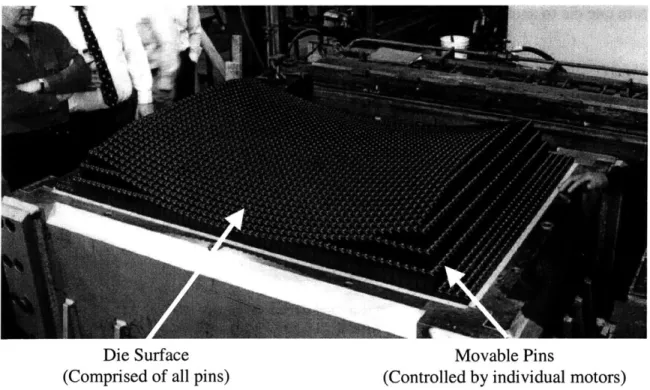
-numerous rigid tools. In part, this was done to reduce the cost associated with die manufacturing, die changeovers, part proliferation, and die storage. The traditional, smooth, rigid die like the one shown in Figure 3-1 is replaced with a re-configurable die created from a grid of spherical tipped, square pins as shown in Figure 3-2 and Figure 3-3. The individual pins that make these dies can be moved independently, which allows this die to change shape.

Figure 3-2: Forming surface of MIT, lab scale, re-configurable tool [Valjavec, 1999]

Die Surface Movable Pins

(Comprised of all pins) (Controlled by individual motors)

To prevent the discrete, die surface of the re-configurable tool from creating 'dimples' in the sheet metal surface, an interpolator is placed between the die and the sheet. The interpolator is an elastomeric material that is used to distribute the contact pressure evenly about the sheet metal to die interface. This prevents the sheet metal parts from taking on a dimpled surface like the die. A drawing representing the placement of the interpolator over spherical capped pins is shown in Figure 3-4. A lubricant, or Teflon sheets are also placed between the interpolator and the sheet metal to reduce the effects of friction. STRETCH FORCE SHEET METAL + STRETCH FORCE

Figure 3-4: Interface between die, interpolator and sheet metal

There are several benefits to using a re-configurable tool. The most visible benefits are reductions in the number of required dies, storage space, and die changeover time. However, the re-configurable tool creates avenues for addressing other problems that have plagued the stretch forming process within the aerospace industry. Die shape can now be adjusted in a much shorter time frame, therefore an iterative approach to defining

springback compensated die geometry may be used to replace or assist resource intensive analytic methods.

Issue # 2: Difficulty in Predicting Correct Die Shape

For developable part geometries, the mechanics of springback can be evaluated with relative ease. However, uncertainties about exact material properties and process parameters limit the usefulness of such approaches in predicting springback compensated die shapes. These situations are complicated further when non-developable shapes are desired. In lieu of analytical methods, die designers have traditionally used experience and guesswork to determine what shape to make a given die. This means that the die development process is typified by time-consuming die rework procedures as shown in Figure 3-5 or poor quality parts when designers are imperfect.

Initial Die Design (FEA, Net Shape, or Guesswork)

Rework Die

Die Manufacture & q

Qualification ₄ Is IDie _No Acceptable? Yes Die Development Complete

I

Figure 3-5: Rework Procedure

In recent years, die design has improved through the use of finite element analysis, which aids design engineers in predicting the correct, compensated die shape. The output plot shown in Figure 3-6 is from ABAQUS, one such finite element analysis program. The

Spring Forward Algorithm developed at MIT [Socrate, 1996] is an approach to die design that relies heavily on the use of FEA. In the Spring Forward Algorithm, a part is formed over a die with the reference part shape in simulation. The elastic springback of the part is measured and then subtracted from the reference part shape. This springback compensated shape is then used as the die shape in a real forming trial. While these approaches are a great improvement over guesswork, they do require significant engineering resources for the design of every die. Their success is also directly tied to the how well the design engineer estimates the specific stretch forming process parameters and material properties that will be used with a given die. Such estimates are difficult to make accurately.

TIRE COMPLETED IN TRI$ ST'EP I .6 D TIME 3.00 ABAQVS VERSrlNh 5.8-12 DATE: 31-JAN-2001 TINE: 12:5Ic29

Figure 3-6: sample output of ABAQUS FEA

An in-process algorithmic approach to defining die shapes is made very attractive by the uncertainty of material and process parameters, and the amount engineering resource required to use FEA techniques effectively. The availability of a re-configurable tool also makes such an approach feasible and relatively easy to implement. It was these

factors that led Webb [1981,1987], Osterhout [1991], and Vaijavec [1999] to the development of the algorithms detailed in this thesis.

Issue # 3: Excessive Shape Variation in Stretch Forming

The third problem is excessive variation in the geometries of produced parts. A lack of standard operating procedures (SOP's) and the choice of methods used to control the stretch forming process create excessive variation in practice [Parris, 1996]. The trajectory of the stretch forming process is often controlled by monitoring the pressure in the machine's hydraulic cylinders, the displacement of the hydraulic cylinder's, or even through the operator's rough, visual estimates of the process. The inherent variation associated with these control methods exacerbates the variation seen in parts formed under such control schemes. Work performed at MIT by Parris [1996] and Valentin [1999] has shown that implementing standard operating procedures and monitoring material strain levels can reduce process variation significantly.

1.2 1 SOP Displacement Control SOP Strain Control E 0 0 0. 0 . 0 0 z 0.8 -0.6 -0.4 -0.2 - 0-No SOP Force Control SOP Force Control

Figure 3-7: Variation levels associated with different process control strategies (SOP: Standard Operating Procedure)

The results of research performed by Andrew Parris [1996] on the variation levels associated with different control schemes are shown in Figure 3-7. The basic argument for using strain control can be explained by viewing the stress strain curve shown in Figure 3-8 [Hardt et al. 2001]. The stretch forming process generally requires all of the sheet metal to be stressed well into the plastic region. The figure depicts how slight variations in stress are associated with much larger variations in strain at these points of the stress-strain curve. When the stretch forming process is operated under force control, it is effectively measuring an integrated stress value over the cross section of the sheet. Minor variations in the measured force level are associated with much greater variations in the corresponding strain state of the material. The opposite is true when strain is measured.

Displacement is sometimes controlled during stretch forming as it is linked to the strain value of the sheet. Controlling displacement can be problematic as it is difficult to discern what portion of measured displacements are associated with the elongation of the sheet metal, and which portions are associated with the flexing of the stretch forming machine structure. Approaches that use displacement control also require significant engineering resources to define trajectories of all of the axes involved with the stretch forming process.

A

Stress variation

Strain variation

Figure 3-8: Stress - Strain curve sensitivities

Summary

The problems associated with stretch forming are classified into three categories. These categories include the large number of dies required, the difficulty associated with die design and the process variation associated with conventional stretch forming control modes. Prior research performed by MIT and Northrop Grumman has addressed these issues through the development of a reconfigurable die that can replace numerous fixed dies. This reconfigurable tool made possible the use of closed loop shape control algorithms for die design, based on an in-process, cycle-to-cycle shape measurement. This research builds on these shape control algorithms. Prior research has also identified control modes that minimize process variation [Parris, 1991; Valentin, 1999]. This becomes critical to the shape control algorithms as it they can sometime amplify process variation [Siu, 2001].

Chapter 4 : The Generic Algorithm Structure

In this chapter, a general framework for all of the closed loop shape control algorithms is presented. This framework is presented graphically, through recursive equations, and through the context of a discrete control system. These frameworks provide a means to quantify the expected performance of the algorithm. Additionally, some implementation issues common to all forms of the algorithm are presented.

Stretch forming process model

A model of the stretch forming process is first developed to help understand how the algorithm attempts to find the appropriate die shape. The stretch forming process is decomposed into the following categories: input, equipment, material, and output. These categories are shown in Figure 4-1. The equipment is further broken down into equipment properties and states, which collectively represent how the stretch forming process applies energy to the material. The material is also defined by its various properties and states, which quantify how material is affected by the energy applied to it. Some of the various equipment and material properties and states are provided in Figure 4-2.

propetes Ma perties OTU

states P- states - Geometry

-Properties

Figure 4-1: Stretch forming process model

Properties Die Geometry Yield Stress

Structural Geometry Elastic modulus Structural Stiffness Strain Hardening Coefficient States Hyd. Cylinder Pressure Net Stress or Strain

Hyd. Cylinder Positions Bending Moment

Controlling the geometry output of this process has been the historical problem and is thus the primary concern of the algorithm. Die geometry is the equipment property with the most impact on the output part geometry. It is also the one property that can be readily controlled through the discrete die. For these reasons, it is chosen as the variable to feedback and modulate in attempts to achieve a desired output geometry. Attempts are made to keep all other equipment/material properties and states constant from one forming cycle to the next in the algorithm. Figure 4-3 depicts errors in the process output geometry (part shape) being fed back to change the equipment property (die shape) in effort to correct the output geometry.

INPUTS Equipment ENERGY Material OTU

- properties -properties -OTry

- -states -states - Peopere -Properties

Geometry

Figure 4-3: Stretch forming process model with feedback

Algorithm Model

Over the past 15 years, the general form of the die prediction algorithm has maintained the same basic structure. However, the algorithm has been applied to different processes by Webb [1981, 1987], Osterhout [1991] and Valjavec [1999]. The goal of the algorithm has always been to find the correct compensated die shape required to form a given part shape. Here, die and part shape are mentioned in generic terms, meaning they can reflect any parameter that is used to define a die or part shape in its entirety, or a collection of parameters used to define the die or part shape.

A flowchart depicting the general concept of the algorithm is shown in Figure 4-4. The process begins by taking the best guess at the appropriate die shape. The best guess can be made with finite element analysis, an evaluation of historical data, intuition or simply by choosing a net shape die as a starting shape. A part is then formed on this die and then

compared to the desired part. If the difference between the desired part and the first formed part (the part error) is within acceptable bounds, the process is terminated and the algorithm is not used. However, if the errors are not acceptable, the die shape is adjusted by a scaled factor of the previous part errors. The scaling factor that is used can be arbitrarily set to a value of unity, or can be defined by knowledge of the appropriate process physics, by historical data, or by system identification techniques performed on similar die and part shapes. A second part is then formed with the updated die shape and differences between the second part and the desired part are measured. The algorithm repeats in this manner until an acceptable part is made.

Make Prediction of Springback Compensated Die

Shape

Stretch Form a Part Predict the

on the Current Compensated Die

Prediction of the with Shape Control

Correct Die Shape Algorithm

no Compare Formed

Part to the Desired _{Is Part Terminate}

Part by Calculating _{Acceptable yes Algorithm}

Errors

Figure 4-4: Block diagram of generic algorithm structure

A recursive equation is constructed to represent this form of the algorithm. It is shown in Equation 4-1. The difference between the target part and a formed part is the part error

(e) as shown by Equation 4-2. This equation can be substituted into Equation 4-1, which produces Equation 4-3.

di = di- _+ g c (Pref - Pi-1 )

Equation 4-1 Or

Idi

1di-1

+

2i-1 2,1 gC 2,2 C 2 Pref 2 i-1

MNd_ MNd-1 MN,1 9c MNMNgC _ MNPref _ MNPi-1_

(MN,1) (MN,1) (MN,MN) (MN,1) (MN,1)

Where:

di = vector representing die shape for the i iteration

p = vector representing part shape for the ith iteration

i = iteration counter

Pref = vector representing reference part shape

gc = matrix of controller gain

It is helpful to view Equation 4-1 in vector / matrix format as shown below it. Here, each collection of die and part variables are contained in a column vector. For example, a die that consists of a grid of M by N pins is sometimes defined by the position of each of its pins. In this case there are M x N pins. While these pins are in a matrix form in the tool, there are shown as a column vector in Equation 4-1. The coefficients of the part and die values define which specific points of the part or they represent.

However, the controller gains are contained in matrix that has dimensions MN by MN. This is because a gain value is needed to relate every part data point to every die data point. The coefficients for these gain values indicate which particular part and die data points that are being related. The primary diagonal of this matrix contains gain values that relate a data point in a part to the corresponding point in the die. The off-diagonal terms related part data points to different die data points. These terms couple the action

e = Pef - P Equation 4-2 Or 2 i .MNei (MN,1) 1

Pref

Pi

e = variable(s) representing error of the i part

di = d _₁ + gcei-1 Equation 4-3 Or 2 9C 1,MNgC 2 9C MNMN gC (MN,MN) + Idi _MNdi_ (MN,1) 1 i-1 2di-I MNdi-1 (MN,1) _MN,1 C x MNei-1 (MN,1)

Or alternatively, the change in die can simply be represented by Equation 4-4. Ad- =gee Equation 4-4 Or 1

Ad

Adi = vector representing change to the i' die

This recursive equation represents the feedback of part geometry information shown in Figure 4-3.

Schematic Process Model

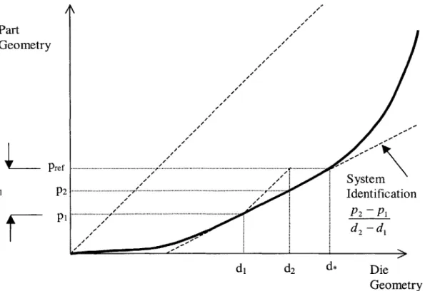
Graphical models can be constructed for cases where one parameter is used to define the geometry of an entire part. Cylindrical parts of constant curvature are examples of this as they can be characterized by their curvature alone. Such a model is shown in Figure 4-5 when the assumption is made that other material and process characteristics remain constant, such as the final strain state or the material properties.

/ d* "d2" is the algorithm predicted die Die Geometry -- Ad,

Figure 4-5: Schematic model of algorithm

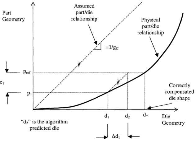
Here the physical relationship between die geometry (d) and part geometry (p) is represented by the thick curve shown in the graph. While this relationship can be determined analytically for developable sheets of constant curvature, it is treated as unknown in this example. The goal is to find the correct die shape (d*) that will create the target part geometry (pre). Because of springback, the line in Figure 4-5 will generally lie below the line with unity slope that crosses through the origin. The first guess at die shape is represented by (dl) and the corresponding part is shown by (p]). The difference between the target part and the first formed part is calculated (el) and then these errors are multiplied by weighting factors (gc) to define how much the die should be adjusted. In this example, the weighting factor(s) are arbitrarily set to unity. The weighting factor (gp) can be interpreted as a guess at the local slope of the physical relationship between part and die geometry. The resulting die prediction is the intersection between the assumed plant gains (gp) and the reference part (pref). This is denoted in the figure by (d2). This figure suggests that an approach that identifies the

Part Geometry Assumed part/die relationship Physical part/die relationship =1/gc Correctly compensated die shape

L

slope of the physical part/die relationship may provide a more accurate prediction (one closer to d*) and converge in fewer trials.

Control system view

The algorithm is now placed into the context of a discrete control system. The discrete control system framework is chosen because it allows us to apply established system analysis tools to the algorithm. This allows algorithm performance to be more easily quantified and also provides some insight as to how the algorithm functions. The framework of this system is shown in Figure 4-6.

prei ei-1

-di_

Controller d- -1 Plant

Unit Delay

pi-I _z-1I Unit Delay

Figure 4-6: Control system view of algorithm

Here the process again begins with (di) being the initial 'best guess' at the die shape. This die is used to create the first part (pi). The stretch forming process is represented by gain factors associated with the 'plant' (gp). With the first part formed, the first cycle of the process is complete. The index is thus changed from (i=1) to (i=2) making the first part (pi.1). This is represented in the schematic by the z-transform unit delay (z-1). Errors

(ei.u) are then calculated for (pi.j), and multiplied by the controller gain factors (gc). The controller uses the errors and its gain factors to define what changes should be made to the die (Adi). These changes are then added to the previous die shape (dt.1) to form the next die shape (di). The additional unit delay in this portion of the schematic represents

the memory the system has of the prior die shape. A new part is formed and the cycle continues.

Steady state error

It is possible to determine whether a steady state error is to be expected from the structure of the control loop. The first step in understanding this is to calculate the closed loop transfer function. This is performed in Equation 4-5 through Equation 4-7.

gcgp

P

The limit of the closed loop transfer function, multiplied by z and the unit step input is then taken as z approaches unity (this is represented by Equation 4-8). The value produced is unity, which means the desired output will match the input and no steady state error is expected. This is possible because the algorithm is adding the errors of the last part formed to those from all previous parts formed. This "integrating" effect allows convergence to a zero, steady state error. It should be noted that the algorithm takes the

limZ(Z-1(Z t c;PZ Z

Z -1+ ggP )Z

Equation 4-8

Response time

The root locus method can be used to understand the effect of system controller gains on the response of the closed loop system. To perform a root locus analysis, the open loop transfer function must first be calculated to create the root locus plot. Equation 4-9 reflects this transfer function.

A- gCgPZ

Equation 4-9

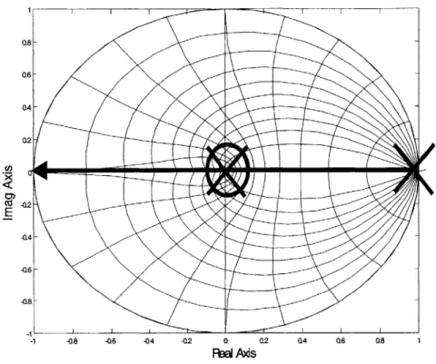
This open loop transfer function has two poles, one located at one and the other at zero on the real axis. However, the pole located at zero is cancelled by the zero in the transfer function, also located at zero on the real axis. This effectively leaves one pole located at one on the real axis. The root locus for all closed loop gain values is thus a line extending toward negative infinity on the real axis as shown in Figure 4-7. This model assumes that gc and gp are system gains without their own dynamics.

I

I--I I I I [ -- -~-~~- ______

Q4 06 Q8 1

Figure 4-7: Root locus of die configuration algorithm

For loop gains ranging between zero and unity, the root locus suggest the response will exhibit an over damped behavior as depicted in Figure 4-8. These points lie on the real axis of the root locus plot between Z=1 and Z=O. The response time will be shorter for closed loop gains closer to unity, which represents points closer to the center of the unit circle. (8 G6 04 Q2 E -Q2 -4 -06 -Q8 -1 -08 -06 -04 -Q2 0 02 FbaI Ms 1

2 1.5 0.5 0 -0.5 -1 -1 0 1 2 3 4 5 8 9 10 6 7 8 9 10 Output (GcGp=0.75) 1 0 1 2 3 4 5 6 7 8 Output (GcGp=1.25) 9 10 1.5 1-0.5 - 00.5 --1 -1 0 1 2 3 4 5 6 7 8 Output (GcGp=0.25) 9 10 Output (GcGp=1) 1 0 -0 .1 -*---~****** .52 -1 0 1 2 3 4 5 6 7 a 9 1 Output (GcGp=1.75)

Figure 4-8: discrete, system responses

A closed loop gain value of unity provides the desired system dynamics of a dead-beat

controller as shown in Figure 4-8. A controller is known as a 'dead beat' controller if it converges in a single iteration. This point lies in the center of the unit circle on the root

locus plot. 1 2 3 4 5 6 7 Input (Impulse) 1.5 0.5 -0.5 1.5 1-0.5 -0.5 -1 0 1 2 3 4 5 6 7 8 9 1 1.5 1 0.5 -0.5 ---1 i 3 0