Application of the method of parametric differentiation to two dimensional transonic flows

by

Woodrow Whitlow, Jr.

S.B., Massachusetts Institute of Technology (1974)

S.M., Massachusetts Institute of Technology (1975)

SUBMITTED IN PARTIAL FULFILLMENT OF THE REQUIREMENTS FOR THE DEGREE OF DOCTOR OF PHILOSOPHY

at the

MASSACHUSETTS INSTITUTE OF TECHNOLOGY September 1979

Massachusetts Institute of Technology Signature of Authot

-Department of'eronautics & Astronautics August 17, 1979 Certified by Thesis Supervisor Certified by_ . Thesis Supervisor Certified by Thesis Supervisor Certified by Thesis Supervisor Certified by_ Thesis Supervisor Accepted by

CU anDepartmental Graduate Committee MASSACHUSETTS INSTUToE

OF TECHNOLOGY OCT

5

by

Woodrow Whitlow, Jr.

Submitted to the Department of

Aeronautics and Astronautics on August 17, 1979 in partial fulfillment of the requirements for the

degree of Doctor of Philosophy ABSTRACT

The problem of unsteady, two dimensional transonic flow is investi-gated. The flow field is modeled using the small perturbation potential equation. Assuming that the unsteadiness can be treated as a linear perturbation about the steady state, the potential is separated into steady and unsteady components. This results in a nonlinear equation for the steady flow and a linear equation, coupled to the steady flow, for the unsteadiness. The problems presented by the nonlinearity of the mean flow are circumvented by differentiating the steady flow equation with respect to either the airfoil thickness ratio or the angle of attack. The nonlinear problem is then reduced to solving a set of ordinary differ-ential equations and a linear partial differdiffer-ential equation with variable

coefficients. A relaxation procedure is uniquely combined with predictor-corrector methods to calculate steady transonic flow fields for various airfoil thickness ratios and angles of attack; free stream Mach numbers less than unity are used in all cases. The data obtained using this method compares well with experimental data and data obtained using other

prediction techniques. The steady flow data is used to determine the effects of varying the airfoil thickness ratio on the unsteady aero-dynamic loads. If shock waves are present in the flow field, a compatability condition is introduced at the mean shock location to account for the effects of moving shock waves. By monitoring the

amplitude of the shock motion, I am able to determine when the assumption that the unsteadiness is a linear perturbation about the steady state is violated. I also present analysis which provides me with an estimate of the maximum reduced frequency of the unsteady motion which leads to stable numerical solutions of the unsteady potential equation.

Aeronautics and Astronautics Thesis Supervisor: Judson R. Baron Title: Professor of Aeronautics and

Astronautics

Thesis Supervisor: Eugene E. Covert Title: Professor of Aeronautics and

Astronautics

Thesis Supervisor: Jack L. Kerrebrock Title: Professor of Aeronautics and

Astronautics

Thesis Supervisor: Marten T. Landahl Title: Professor of Aeronautics and

The completion of any major project is very seldom the result of the efforts of a single individual, and credit should be given to those who took interest in and assisted the individual whose name

adorns the the final report. Many thanks are due Professors Judson R. Baron, Eugene E. Covert, Jack L. Kerrebrock, and Marten T. Landahl for their helpful suggestions and criticisms throughout the course of this research effort. Dr. William T. Thompkins also deserves thanks for his valuable advice on numerical methods.

It is very difficult for a student to make a significant contribu-tion to his field of specialty without a positive force to guide him. In this case, I would like to recognize the support and other intangibles given to me by Professor Wesley L. Harris - a close friend who happened to be my thesis chairman. Space does not permit me to list the many ways in which he has made my MIT experience a more meaningful and enjoyable one.

The role of the family cannot be overlooked, and I would like to begin by thanking my mother and father, Woodrow and Willie Mae Whitlow, for both their moral and financial support. I must give my heartfelt thanks to those who had to endure perhaps more than I - my wife, Michele, and daughters, Mary and Natalie. Michele deserves special praise for her financial and spiritual support and for typing this manuscript.

Special thanks are also due Dr. Jerry Bryant and Earnestine Bryant for helping me to keep the entire MIT experience in perspective. The following friends also deserve mention: Ali Ahmadi, Briggette Bailey,

Kenneth Leighton, Luiz Lima, Rudolph Martinez, Dr. Tom Matoi, and Karen Scott. Gloria Payne deserves special thanks for her efforts.

The National Aeronautics and Space Administration (NASA) supported this work under NASA Grant NSG 1219, Dr. Samuel Bland, Technical Monitor. The stimulating discussions with NASA employees Dr. E. C. Yates and

Dr. Perry Newman are greatly appreciated. Some financial assistance was also obtained from the Office of the Dean of the Graduate School

at MIT. All computations were performed at the MIT Information Processing Center as Problem M12702.

Chapter

Figure

2.1 Geometry of curved shock waves

Page 13 22 44 57 96 125 Appe 1 Introduction

2 Formulation of the Problem of Unsteady Transonic Flow Past Airfoils

3 Analysis of Steady, Two Dimensional Transonic Flows

4 Determination of the Rate of Change of the Steady Potential and Results for Steady Flows

5 Solution Procedure and Results for Unsteady Flows

6 Conclusions and Recommendations ndix

A Predictor-Corrector Methods for Generating Starting Solutions

B Base Solution for Nonlifting Biconvex Airfoils C Finite Difference Equations for the Rate of

Change of the Steady Potential

D Finite Difference Equations for the Unsteady Perturbations

E Far Field Conditions and Evaluation of the Wake Integral

F Stability Analysis and Frequency Limitations G Tridiagonal Matrix Solver

H Fortran Programs 130 134 136 156 171 185 190 195 28

2.2 Region traversed by imbedded shock wave 33 2.3 Typical perturbations about the steady state 37

airfoil position

2.4 Location of the cut in the flow field 39 2.5 Imbedded supersonic region and shock wave in a 41

transonic flow field

3.1 Solution procedure using the method of parametric 50 differentiation

4.1 Regions of the physical plane 60

4.2 Typical transformed coordinate system 60

4.3 Full plane boundary value problem 65

4.4 Half plane boundary value problem 66

4.5 Element of area in the computational plane 68 4.6 Grid spacing near the airfoil trailing edge 76 4.7 Pressure distributions on nonlifting parabolic 77

arc airfoils at M = .825

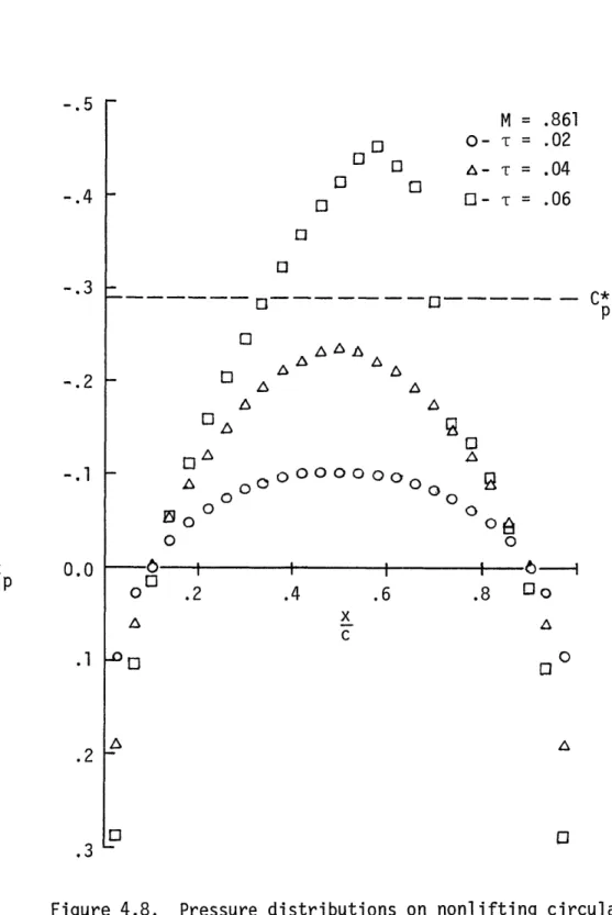
4.8 Pressure distributions on nonlifting circular 78 arc airfoils

4.9 Computational requirements for nonlifting parabolic 79 arc airfoils

4.10 Computational requirements for nonlifting circular 79 arc airfoils

4.11 Pressure distributions on a six percent thick, 82 nonlifting circular arc airfoil

4.12 Pressure distributions on a six percent thick, 83 nonlifting parabolic arc airfoil

4.13a Pressure distributions on a lifting circular 84 arc airfoil

4.13b Pressure distributions on a lifting circular 85 arc airfoil

circular arc airfoil at M = .806

4.14b Moment coefficients about the leading edge of a 86 six percent thick circular arc airfoil at

M = .806

4.15 Computational requirements for lifting circular 87 airfoils at M = .806

4.16a The jump in g at the airfoil trailing edge and the j₈mp 88 in g used to evaluate the far field; M = .806, a = 0

4.16b The jump in g at the airfoil trailing edge and the jgmp 89 in g used to evaluate the far field; M = .806, a =.6

4.16c The jump in g at the airfoil trailing edge and the jgmp 89 in g used to evaluate the far field; M = .806, a 1

4.17 Pressure distributions on a six percent thick 91 circular arc airfoil

4.18 Pressure distributions on a six percent thick 92 parabolic arc airfoil

4.19 Pressure distributions on a six percent thick 93 circular arc airfoil

4.20 Pressure distributions on a six percent thick 95 parabolic arc airfoil

5.1 Unsteady boundary value problem 102

5.2 _{Location of the imbedded shock wave, relative to 110} the computational grid

5.3a _{Unsteady lift distribution on a flat plate oscillating 113} in heave

5.3b _{Unsteady lift distribution on a parabolic arc airfoil 114} oscillating in heave

5.3c _{Unsteady lift distribution on a parabolic arc airfoil 115} oscillating in heave

5.4 _{Unsteaay lift coefficients and moment coefficients 116} about the leading edge divided by the amplitude of

5.5a 5.5b 5.5c 5.6 5.7 5.8 E. 1 E.2

I Shock motions for a circular arc in heave at M = .861

airfoil oscillating II Shock motions for a circular arc airfoil

in pitch about its midchord at M = .861 III Shock motions for a circular arc airfoil

in pitch about its midchord at M = .861

oscillating oscillating References

Unsteady lift distribution on a flat plate oscillating in pitch about its midchord

Unsteady lift distribution on a parabolic arc airfoil oscillating in pitch about its midchord

Unsteady lift distribution on a parabolic arc airfoil oscillating in pitch about its midchord

Unsteady lift coefficients and moment coefficients about the leading edge divided by the amplitude of oscillation for pitching parabolic arc airfoils

Unsteady lift distribution on a circular arc airfoil oscillating in heave

Unsteady lift distribution on a circular arc airfoil pitching about its midchord

Area and path of integration and local normal to the path of integration

Gaussian integration procedure

117 118 119 120 121 122 172 184 Table 124 124 124 281

(a - Speed of sound

- Exponent of M in the nonlinear term of the steady potential equation

C - Airfoil chord length - Pressure coefficient

- Critical pressure coefficient - Lift coefficient

C - Moment coefficient about the airfoil leading edge

- Mean airfoil position

- Perturbation about the mean airfoil position

- _ or -..f

A4 -6 Y

- Unit vector in the streamwise direction

w ,

- Unit vector in the direction normal to the free stream - Free stream Mach number

- Pressure

- Magnitude of the velocity vector

- Specific entropy

7/ t - Time

7- - Temperature

LA - Velocity vector U - Free stream velocity

X,. - Unstretched coordinates in the streamwise direction - Instantaneous shock wave position

- Shock excursion amplitude - Mean shock wave position

- Unstretched coordinates in the direction normal to the free stream

- Angle of attack

0(0- Mean angle of attack

- Ratio of specific heats - Circulation

- Amplitude of unsteady motion - Characterizing parameter 46 - Increment in i

'? - Stretched coordinate in the direction normal to the free stream

A 7 - Coordinate spacing in the ' direction - Unsteady shock motion

- 3.14159... - Density

- Measure of camber and angle of attack - Airfoil thickness ratio

-Perturbation velocity potential - Steady component of f

-Unsteady component of ( - Amplitude of i

- Velocity potential

- Relaxation factor; frequency in the definition of - Vorticity vector

Subscripts

13

- Denotes free stream conditions

CHAPTER I INTRODUCTION

The aerodynamic forces acting on aircraft operating at transonic speeds are generally greater than those acting on aircraft in subsonic or supersonic flight. When aircraft undergo unsteady motions while operating in the transonic flight regime, disturbances interact and build up, and there may be large phase differences between the aircraft motion and its unsteady aerodynamic loads. These characteristics make it more likely that flutter and other dynamic instabilities will occur in transonic flight. Hence, in this age of high subsonic and supersonic aircraft, the behavior of flight vehicles while operating at transonic speeds is of great concern to aircraft designers.

In order to design a vehicle that can operate safely at the desired flight conditions, we need the ability to determine the steady and

unsteady airloads on aircraft in transonic flight. One way to accom-plish this is to use the wind tunnel as a design tool, but the cost of models and wind tunnel test time will most likely result in the choice of a configuration that does not possess the optimum aerodynamic

characteristics. Consequently, we should seek to develop methods to predict the aerodynamic loads acting on aircraft in transonic flight.

The primary difficulty associated with predicting transonic flow fields is that the governing equations are nonlinear and that, generally, various types of flow regions and shock waves are present in the flow field. Early studies of steady, two dimensional transonic flows avoided

the problem of nonlinearity by using the hodograph method [1]-[3]. The governing equations become linear in the hodograph plane, but the method is limited because of the difficulty of satisfying the boundary condi-tions for general airfoils. Hence, only simple wedge profiles were considered in those early studies. More recent studies show that hodograph methods are quite useful for treating the inverse problem of transonic airfoil design [41,[5].

Because of the limitations of the hodograph method when applied to direct problems, it was necessary to develop other transonic methods. Spreiter and Alksne [6] developed the method of local linearization to

solve the steady, two dimensional, transonic small perturbation potential equation. However, the assumptions upon which that method is based

limits its applicability to flows with free stream Mach numbers at or very near unity. Hence, local linearization is restricted to analyzing flows in a narrow portion of the transonic Mach number range.

Landahl [7] described the unsteady transonic flow field with a small perturbation potential equation and separated the potential into steady and unsteady components. He demonstrated that for high frequency motions in near sonic flow the unsteady potential equation is linear

and uncoupled from the nonlinear steady flow. In that form, analytic solutions of the unsteady transonic problem were obtained, but, for many problems of engineering interest, low frequency motions must be con-sidered. We are then faced with solving a linear equation with variable coefficients. Additional difficulty arises because those coefficients must be determined from the solutions of the nonlinear steady potential

equation.

One of the most important breakthroughs in transonic flow research was made when Magnus and Yoshihara 18] used a modified Lax-Wendroff difference method to numerically solve the unsteady, two dimensional Euler equations. The steady aerodynamic loads acting on airfoils were then determined by allowing the unsteady solutions to approach a steady state. By obtaining steady state solutions in that manner, it was necessary to solve a hyperbolic equation instead of the more difficult mixed elliptic/hyperbolic equation that results when the steady Euler equations are considered. The computations were lengthy, requiring as much as three and one half hours on a CDC 6400, but the emphasis was on understanding the flow field and not on computational speed. The predicted pressure distributions on a shockless airfoil in

super-critical flow showed good agreement with experimental data except near the supersonic flow region. Also, except where the shock wave and bounda-ry layer interact, the predicted pressure distributions on a NACA 64A410 airfoil in supercritical flow showed good agreement with experimental data. Most important was that the great potential of computational fluid dynamics was demonstrated.

The next major breakthrough came when Murman and Cole [91 developed a relaxation method to solve the steady, two dimensional, small pertur-bation potential equation. That method yielded numerical solutions of mixed transonic flow fields in an order of magnitude less computer time than the method of Magnus and Yoshihara [8]. The Murman-Cole method introduced the concept of type dependent differences, which amounts to

introducing an artificial viscosity into the potential equation at supersonic points. Numerical solutions of the transonic potential equation are continuous throughout the flow field, and shock waves appear as narrow regions with steep gradients. Hence, shock waves are spread over a finite number of grid spaces, and, by allowing the grid spacing to approach zero, the shock thickness can be made arbi-trarily small. Murman and Cole [9] calculated pressure distributions on nonlifting circular arc airfoils, and the agreement with experimental data was very good. Unfortunately, there was no attempt to compare with the data generated by Magnus and Yoshihara [8]. The Murman-Cole method [91 does not maintain conservative form immediately downstream of shock waves and does not enforce the theoretical shock jump conditions, but this was corrected when Murman [101 developed a conservative type dependent difference method.

Following the success of Magnus and Yoshihara [8] and Murman and Cole [9], research in the field of transonic aerodynamics intensified, as evidenced by the frequent appearance of review papers in the

literature [41,[11]-[14]. Jameson [15] performed a von Neumann test which indicated that the Murman-Cole difference method [91 has a marching instability in the streamwise direction if the flow is not perfectly aligned with the coordinate system (However, the Murman-Cole method has worked extremely well in practice). He then introduced a rotated difference method for solving the full potential equation. This method was unique because no assumptions about the flow direction were made. Jameson [16] later developed a conservative rotated difference

method for the full potential equation which demonstrated excellent agreement with experimental pressure measurements on blunt nosed

airfoils.

Another improvement in transonic flow calculations, but not as significant as the breakthroughs of [8],[9] and [15], was made by Ballhaus and Goorjian [17] when they applied an alternating direction implicit (ADI) method to the low frequency small perturbation potential equation. Ballhaus and Goorjian [171 presented results that compare very well with those of Magnus and Yoshihara [8] and require sub-stantially less computer time to obtain.

Following the lead of Landahl [71, several researchers sought solutions of the separated unsteady small perturbation potential

equations [18] -[23]. The steady component of the flow field is governed by a nonlinear equation, and the unsteadiness is described by a linear equation which is coupled to the steady flow. Stahara and Spreiter [18], [19] and Isogai [201 have applied the concept of local linearization to the unsteady potential equation, but the analysis restricts the applica-bility of the unsteady local linearization method to flows with sonic or near sonic free stream velocities. Hence, numerical methods were applied to the separated potential equations.

Ehlers [21] and Traci et al. [22],[23] developed finite difference methods to solve the separated unsteady potential equation, but none of those methods accounted for the effects of unsteady shock wave motions. The experiments of Tijdeman and Zwaan [24],[25] indicate that moving shock waves induce relatively large local pressures on the portion of the

airfoil over which they travel. When the pressure distributions are integrated over the airfoil chord to yield the unsteady aerodynamic loads, the importance of considering the unsteady shock wave motions becomes apparent. Hence, we should hesitate before using the results of [21]-[23] in stability calculations and should seek to improve those methods.

The present research effort is aimed at developing an efficient tool that can be used to predict the onset of flutter and other insta-bilities. In this study, I employ the concept of a separated small perturbation potential. In order to determine the stability

boundaries, many solutions of the nonlinear steady flow equation may be required, and a method to efficiently determine those solutions is needed. Nixon [26],[271 developed a perturbation method which may be used to determine steady flow solutions for various free stream Mach numbers and airfoil conditions. That method is somewhat limited because the steady flow conditions cannot be changed if the change causes the appearance or disappearance of shock waves. Hence, I seek to

develop a method which can be used to efficiently determine steady transonic flow fields and not be subject to the type of restrictions that Nixon [26],[27] faces.

To determine the necessary steady flow fields, I employ the method of parametric differentiation, which was first used to predict steady transonic flow fields by Rubbert and Landahl [28]. This method reduces the nonlinear steady potential equation to a set of ordinary differential equations and a linear partial differential equation

describing the rate of change of the nonlinear solution with a chosen physical parameter. By integrating the ordinary differential equations over a range of parameters, I easily obtain a number of solutions of the steady potential equation. The primary difficulty associated with this technique is that I must solve the linear partial differential equation for the rates of change of the steady solution with the chosen parameter.

In this study, I develop a relaxation procedure to determine

the rate of change of the steady potential with airfoil thickness ratio and angle of attack. The rates of change of the potential with airfoil thickness ratio and angle of attack are described by the same equation, with only the parameterized tangency condition differing. Thus, the same numerical procedure is used to compute both rates of change of the solution.

At each point in the flow field, the relaxation solutions are uniquely combined with a predictor-corrector method to integrate the steady solution in the direction of the chosen parameter. Nixon's perturbation method [26],[27] differs from this approach in that he expands the potential in a small parameter and obtains an expression relating the velocities for various values of that parameter. However, Nixon is still faced with solving a nonlinear equation for the zeroth order solution; this is not necessary with parametric differentiation. Parametric differentiation also has the advantage of being able to yield both subcritical and supercritical solutions in one

The shock jump conditions in parameter space are satisfied by using conservative type dependent differences. Yu and Seebass [29] and Hafez and Cheng [30] developed shock fitting methods which could give sharp shock wave definition even on coarse grids. They also argue that shock fitting should be used for supercritical flow

calculations because the governing equations cannot always be written in conservation form. However, because of the simplicity of the shock capturing method and because the equation describing the rate of change of the steady solution is easily put into conservation form,

I satisfy the shock jump conditions by using conservative type dependent differences.

Once the steady solutions are known, the unsteady component of the flow field may be computed. The unsteadiness is assumed to vary

harmonically with time which reduces the unsteady problem to a time independent one. Hence, the same relaxation method used to determine the rate of change of the steady solution with the chosen parameter can be used to compute the unsteady component of the flow field. To account for the effects of moving shock waves, I enforce a compatability condition at the mean shock wave location.

In order to demonstrate the present method, the steady forces and moments on lifting and nonlifting biconvex airfoils are computed for free stream Mach numbers less than unity. The computations required to obtain the families of steady solutions are quite reasonable. Having determined the steady state solutions, families of low frequency unsteady solutions are determined. The unsteady solutions allow me to determine

the effects of varying the steady state conditions on the unsteady aerodynamic loads. Hence the methods developed in this study should prove useful as a tool for predicting the occurrence of aerodynamically induced instabilities.

CHAPTER II

FORMULATION OF THE PROBLEM OF UNSTEADY TRANSONIC FLOW PAST AIRFOILS

2.1. Introduction

In order to fully treat unsteady transonic flows, I should be capable of solving for the flow field variables

while considering viscous effects and the fact that transonic flow fields are generally mixed- s-ubsonic and surersonic flow

regions coexist. However, instead of solving the full conservation and state equations, we can obtain most of the essential features and much information about the flow field from the solution of a single, nonlinear small perturbation potential equation. This equation is derived, following Ashley and Landahl [31] from the Eulerian gas dynamic equations by satisfying conservation of mass, linear momentum, and energy to lowest order and assuming the flow to be inviscid, isentropic and irrotational. A major advantage in using the idea of small perturbations is that it allows a simplified treatment of the airfoil boundary conditions; the boundary

conditions may be applied on a mean profile line and expressed in terms of vertical perturbation velocities and local airfoil slopes. Consequently, no special procedure is required to obtain data on the airfoil boundary.

In this chapter, I derive the nondimensional small pertur-bation potential equation and the associated initial and boundary

conditions. The problem is then simplified by separating the potential into steady and unsteady components. The limits on the amplitude of the unsteady motion which allow this separation are determined from a dimen-sional analysis of the unsteady shock motion. The separated potential equations and' te associated boundary conditions are presented. Also, limitations of the small perturbation potential approach are discussed. 2.2. Derivation of the Small Perturbation Equation and Airfoil

BoUndaU . nditions

Because of the assumption of inviscid , isentropic, irrotational flow, the unsteady transonic flow problem can be reduced to one of solving a single equation for a velocity potential, ' . That

equation is derived here following the procedure of Ashley and Landahl [31].

From the equations of conservation of mass, linear momentum , and energy, I can deduce Bernoulli's equation

~

f(2.1)

IT 2

Using Leibnitz's rule to differentiate the integral term in (2.1) yields

P

p

Row, I can write /* where '~

7

'6e.v

4.

To complete the derivation,

J

P

I rewrite Bernoulli's equation

J/p

which becomes, when combined with (2.3)

az:

-

(A

2

Introducing this expression for / lf into the mass conservation

7* i& equation

V')

7-I obtain the full potential equation

-Z-which in expanded form is

- 13 fJ +ZYgy+ 4 T -- , .) = 0 (2.5)

I , next, seek to reduce the complexity of this equation.

The full potential equation may be simplified by assuming the velocity field to be the combination of a uniform stream and perturbations upon that stream. Thus, the potential may be written as

(2.6) where is the perturbation velocity potential. Equations (2.4 ),

(2.5 ) and (2.6 ) are then combined to yield the perturbation potential equation

M ~ z gt/ _2U " 7z

+I +2/+Pr ) i _{L (2.7)}

I may simplify

(

necessitating the retention of the M*/) S tem. When the reduced frequency of the unsteady motion is of order unity, the

term should also be retained. Using the above assumptions, (2.7) is reduced to the transonic small perturbation potential equation

I >;-gl'P)r - M'- It !F 16 r7

Introducing the following nondimensional variables

I obtain the dimensionless form of the transonic small perturbation potential equation

L - -nZ/5s/)4i? - i$-2 -2in2 xI

-!4,.~f

It is essential that any transonic method be capable of accurately predicting mixed flow fields, and even though (2.8) is a simplified flow model, it is capable of yielding mixed flow solutions. However, the small perturbation approach does have some limitations.

One limitation is that the small perturbation assumptions are violated at airfoil leading edges. Ballhaus [141 reports a dependency of numerical solutions on the spacing of the computational grid near

the leading edge. Fortunately, the grid dependency may be confined to a small region near the leading edge by using a fine grid in that region.

A limitation on the geometry of shock waves is seen by considering the curved, adiabatic shock wave of Figure 2.1. Crocco's theorem states

where s is the specific entropy, h₀ is the stagnation enthalpy, T is temperature, 5 is the velocity vector, and i~ is the vorticity vector.

If the upstream flow, u₁ , is steady and uniform, the local vorticity,W%, immediately downstream of the shock wave is

wheref/ is the local shock inclination,

f,

4

Crocco's theorem shows that vorticity is generated in unsteady flows even if there are no entropy gradients. If the velocity field and its rate of change with time are such that significant amounts of vorticity are generated, I can no longer assume potential flow. The actual limita-tion on the level of unsteadiness can be determined by comparing potential flow data with experimental data or data obtained from a flow model that is valid for both rotational and irrotational flows. When the potential flow data begins to deviate significantly from the experimental data or the data from the rotational flow model, I can assume that the limit on the level of unsteadiness has been reached.

u 1

r

shock waves in the flow field must be sufficiently weak. The increase in entropy, 4s, across a normal shock wave is, [321

3 >,

Usually, when M becomes greater than 1.3, the shock wave separates the boundary layer, and viscous and rotational flow effects must be considered. This result indicates that potential flow models can only be used to

compute flows with relatively weak shock waves. The above result also provides an estimate of the entropy jump across shock waves which causes the potential flow assumptions to be violated.

Because the small perturbation equations are derived assuming that M is nearly unity, there are cases when the predicted flow field may be

in error. A comparison of the critical pressure coefficient, C ,

determined from the exact and small perturbation equations indicate that if M is considerably less than unity, small perturbation theory may pre-dict a completely subsonic flow field when, according to the exact

equations, the flow has become supercritical. Krupp [331, for the case of steady flow, has rewritten the coefficient of as /-M2-Nba1)f,

which allows the choice of b such that the small perturbation approxi-mation of either C* or the average pressure across normal shock waves

p

matches the exact quantities. In this study, b has been set at 2, but as M nears unity, the choice of b becomes less important.

The condition which must be satisfied at the airfoil boundary is determined by considering the airfoil as a streamline across which no fluid flows. Therefore, on the airfoil, the fluid.-velocity

normal to the airfoil must equal the airfoil velocity normal to itself.

If the instantaneous airfoil position is given by

b(X, , 4) = 0 (2.9)

the fluid velocity normal to the airfoil is (/+f)3, ,

and the velocity of the body normal to itself is -.

Hence, the airfoil tangency condition is

t

Generally, for thin bodies x is much less than unity, and the tangency condition may be reduced to

8

t

le Bi = o

Other conditions which must be satisfied are continuous pressure and normal velocity in the wake and the Kutta, shock jump and

far field conditions. How these conditions are treated is detailed in the next sections.

Once I solve (2.8 ) subject to the appropriate conditions, the results are reported in the form of a pressure coefficient,

where

approximation of

4,

(-P = -?-Off- A4) (2.11)

The forces and moments acting on the airfoil are then easily found by integrating the profile pressure coefficient over the chord.

2.3. Separation of the Small Perturbation Potential

For some subsonic and supersonic flows, for which the governing equations are linear, the potential may be separated into steady and unsteady components , each independent of the other. The

transonic equation is nonlinear and, generally, cannot be separated in that manner. However, if the unsteadiness can be treated as a linear perturbation on the steady flow, the transonic potential may also be separated. Here, I use a dimensional analysis and the experimental results of Tijdeman and Zwaan [24 1, [25 ] to determine the conditions under which separation of the transonic potential is allowed.

If I am to be justified in separating the potential in ( 2.8), the unsteady loads should vary linearly with the amplitude of the unsteady motion, with a phase shift. As a result, I must pay close attention to the motions of imbedded shock waves. Shock

waves induce relatively large pressures in the regions over which they travel. Therefore, if tne motion of a shock wave carries it over a

significant portion of the airfoil, the aerodynamic .oads become a nonlinear function of the unsteady motion. I, then, must examine the factors which contribute to the motion of embedded shock waves.

The parameters governing the ratio of the shock excursion amptitude to chord, &x, _{, illustrated in Figure 2.2 are obtained} from a dimensional analysis. I write dxs as a function of the dimensional physical parameters which describe the flow field

where in the above equation, T represents the maximum airfoil thickness. In terms of basic quantities, the shock excursion amplitude becomes

L

.(L"

L e

L

L" L'

L6)

from which I obtain the following relationships

de4

Using the above equations to eliminate two of the variables and then grouping terms with like exponents, the dimensionless dependence of the shock excursion amplitude is formed

4 -(

L((2.12)

s

e c

Equation (2.12) is rewritten as -- ~ c/

where has been used. The experiments reported in

[241 and [251 may be used to determine the

effect of the various nondimensial parameters on A)'$ C

The experiments of Tijdeman and Zwaan show that the shock motion increases when the motion frequency decreases. The shock

excursion to chord ratio is then written as

' /(2.13)

where

6

require <<ze a. if the unsteadiness is to be treated as a C

linear perturbation about the steady state. When o(r,) C

the transonic potential cannot be separated unless some additional constraint, such as high frequency, is met.

Considering unsteady motions for which , the equations governing each component of the flow field are obtained by separating the potential in the following manner

assuming that

4

16i- zc (2.15)

-M ) 4_Xx

-(2.16)

The effects of thickness, camber, and mean angle of attack may be found from (2.15), while (2.16) represents the effects of the unsteady motion.

Although (2.14) is allowable only if_& Z Z,, solutions of (2.15) and (2.16) may be used in problems of engineering interest. For example, flutter prediction requires the analysis of unsteady motions of infinitesimal amplitude. However, because the unsteady flow is coupled to the steady flow, it may be required to obtain a large number of steady flow solutions to predict

specify the complete boundary value problems for each flow component. 2.4. Definition of the Boundary Value Problems

2.4.1. Steady Component

As a consequence of (2.14), the instantaneous airfoil position may be written as

with '3 > . Figure 2.3 shows a typical perturbation about some mean position. Equation (2.9) becomes

B~~x~g,4)e

=g

and the tangency condition which must be satisfied by the mean flow is

( -e = 7ew )

Generally, for thin airfoils, the boundary doesn't vary significantly from the chord, and the tangency condition may be applied on the mean profile line. Thus, the tangency condition is simplified to

, =

7

"x)

The condition that the perturbation velocities vanish in the far field is

(2.18) 9 = / , )

Perturbed Positions

Steady State Position

Figure 2.3. Typical perturbations about the steady state airfoil position.

The conditions expressed in (2.17) and (2.18) aren't sufficient to make

9

The insertion of an airfoil -into the flow field converts it to a doubly connected region, and a cyclic constant is needed to make

4

#

velocity at sharp trailing edges is finite, producing a smooth joining of the upper and lower portions of the flow. Continuous

motion can only occur if there is no pressure discontinuity at subsonic trailing edges. This is simply a statement of the Kutta condition. From (2.11), the steady, small perturbation approximation to the

Kutta condition is

,1#K= (0, j :o) (2.19)

where a represents the jump in a quantity across the line ?= 0. Because there is no mechanism by which oncoming supersonic flow can adjust itself to the presence of the trailing edge, the pressure

is not required to be continuous at supersonic trailing edges. Across the cut in the flow field, pressure and normal velocity must be continuous. These conditions take the form

( X 76 1Z0) (2.20)

(2.21)

N

iA

/

Cut in the flow field

CA)

Using (2.2o) and (2.21), I can write

,4o (2.22)

where the subscript T represents quantities at the trailing edge. If the flow is supersonic at the trailing edge, I require

#(xcc)= 4O -=4(,=0) (2.23)

Where e. is the location infinitesimally downstream of the trailing edge.

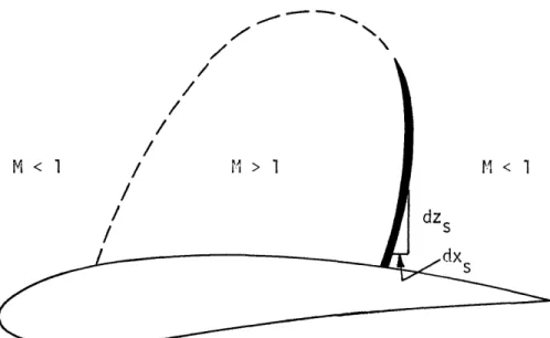
The conditions expressed in (2.17)- (2.23) are sufficient to uniquely determine the flow field in the absence of imbedded shock waves. The appearance of shock waves in the flow field, which is illustrated in Figure 2.5, requires me to ensure the continuity of

#

already contained in (2.15). By writing (2.15) in the conservation form

I t -tyz ) z (+1 Q

(

M < 1 /M> I < 1

dz s dxs

Ns

Figure 2.6. Imbedded supersonic region and shock wave in a transonic flow field.'

is found to be,

<jI~Z)9 2

1raL>(f,)

where < > represents the jump in a quantity across the shock wave. 2.4.2. Unsteady Component of the Flow

At the airfoil, the condition which must be satisfied by the unsteady potential is

A

-g fix (2.25)

In the far field, I require the disturbances to propagate outward without reflection, and at subsonic trailing edges, the Kutta condition requires that

/|($~- x: 2-a '='0 (2.26)

For unsteady motions of high reduced frequencies, experiments have shown that the unsteady pressure at the trailing edge is nonzero [ 34 ], [ 35 1; this nonzero trailing edge loading has been attributed to viscous effects [35 ]. However, for the reduced

frequencies under consideration in the present work, experiments support the validity of using (2.26). Again, if the flow is super-sonic at the trailing edge, there is no requirement of continuous pressure.

Across the wake, the unsteady pressure and normal velocity must be continuous. Assuming the unsteady motion to be small enough such that I can satisfy the wake conditions along the line downstream of the mean trailing edge location, those conditions become

c)

+ (2.27)

A

A T(2.28)

Equations (2.27) and (2.28) imply a discontinuity in 'in the wake. If the trailing edge flow is subsonic, that discontinuity is determined such that the unsteady Kutta condition is satisfied.

The conditions which must be satisfied across imbedded shock waves are detailed in Chapter five.

2.5. Summary

The conservation and state equations have been reduced to a single small perturbation potential equation. The perturbation potential has been separated into steady and unsteady components, with appropriate

boundary conditions specified for each component. From (2.16), it is seen that the unsteady component of the flow field is coupled to the mean

flow. Hence, many steady solutions may be required to predict stability boundaries. The major difficulty in solving for the steady flow is that a nonlinear partial differential equation must be solved. This

non-linearity is essential if mixed flows are to be computed. I have also recognized some of the limitations of the small perturbation approach and presented possible methods to ease those limitations.

CHAPTER III

ANALYSIS OF STEADY, TWO-DIMENSIONAL, TRANSONIC FLOWS 3.1. Introduction

As shown in Chapter two, the separation of the potential simplifies the mathematical complexity of the transonic problem, but many steady state solutions may be needed to fully predict the unsteady responses of bodies in transonic flow. As a result, we

would be required to repeatedly solve a nonlinear partial differential equation, subject to various steady state boundary conditions. Thus, I seek a method which will allow us to easily calculate steady

transonic flows over a wide range of conditions. One such method is the method of parametric differentiation.

Parametric differentiation is a procedure by which certain nonlinear problems, which are characterized by some physical parameter, may be transformed into linear problems by considering the perturbations about a known base solution due to small changes in that parameter. The effects of large parameter changes

are found by repeatedly incrementing the parameter in small amounts. Hence, from the linear equations, I may obtain many nonlinear

solutions as a function of the physical parameter. The chosen parameter may appear in the governing equations and/or the boundary or initial conditions.

and has been previously applied to a wide range of problems in fluid dynamics. Rubbert and Landahl applied the method to the Falkner-Skan boundary layer problem and to the problem of steady transonic flow past nonlifting airfoils [28 ],[36

1,

1,

1

In this chapter, I outline the method of parametric different-iation and present the formulation of the steady transonic boundary value problem in parameter space. I demonstrate that application of parametric differentiation to the transonic problem reduces it to a set of linear, independent first order ordinary differential equations with the base solution as an initial condition. A technique

for solving ordinary differential equations is then employed to extend and determine the potential for various values of the parameter of in-terest. I also present a procedure for determining the base solution. 3.2 The Method of Parametric Differentiation

In order to understand the concept of parametric differentiation, consider a function,

1(Xt;

/V ) C 0(3.1)II (;l t;6

and satisfies the boundary conditions

d,' ) 8 (3.2)

where /\ is a nonlinear differential operator, X. is the boundary

location, and 4 is a characterizing parameter. By differentiating (3.1) and (3.2) with respect to

e

S'4(3.3)

where L is a linear differential operator, and , the increment in the solution due to a small change in the parameter is defined as P_ . Generally, the linear operator will have variable

coef-dE

ficients involving 0 and its derivatives, thus the primary

dif-ficulty becomes to solve a linear equation with variable coefficients. The method of parametric differentiation is not the ideal method for all nonlinear problems, and before I decide to apply

the method to any problem, I should be certain of the following (a) The governing equations become linear

(b) The results are physically plausible (c) The method is cost effective

(d) Extended solutions are weak functions of the base solution

This final point is particularly important. For most problems, a base solution is easily obtained, but in some cases, the perturbations about the base solution may be singular. In such cases, Rubbert and

Landahl [28 ] suggest starting from an assumed solution for 6

=6,-4A6.

Even though that starting solution may be slightly incorrect, if the extended solutions are indeed weak functions of the base solution, we will obtain the correct solution when 6 becomes only slightly

different from its starting value.

3.3. The Steady Transonic Problem as an Ordinary Differential Equation

Upon application of the method of parametric differentiation, at every point in space, the steady transonic flow problem is re-duced to the initial value problem

.6.) , (3.5)

where , is the base solution. Numerical techniques for solving ordinary differential equations may be applied to (3.5), and entire flow fields for various values of 6 are obtained in one integration of the differential equation.

Some of the most successful and widely used techniques for integrating ordinary differential equations are the Runge-Kutta methods. To determine #(e,+46) using the Runge-Kutta

methods, it is required that be known in the interval 6,+4.

Because it is inconvenient to obtain data in the interval , 5,*d,, I chose not to use Runge-Kutta methods to solve (3.5). One method which does not require knowldege of in the aforementioned interval

is the Euler, or tangent line method Z(61+*,

k #(,)+ 64}(4) (3.6)

This method assumes that, throughout the interval o , the solution follows a linear path tangent to 0(4), and its error is proportional to 661. Since Euler's method extends the solutions using a linear approximation and its error term is relatively large, the solutions would have to be extended in relatively small increments to maintain accuracy. Hence, Euler's method is not used to solve (3.5), and a desirable multistep method is sought.

Equation (3.5) is integrated using a fifth order predictor-corrector method [41]. The procedure is to start the solution with the lower order methods given in Appendix A and predict the

next solution with Milne's predictor

C+4 ) 9I6-.?4 ) - 4 e42}14)}-4 jel( ) -2e7

3

+ 14 d,5 (3.7)

The predicted soultions are then modified with the relationship

'{16 ?) CP/1-6) .i/Z [66) -pc6) (3.8)

where C6() is the corrected potential at the previous integration step. The values of m from (3.8) are used as potentials to define the coefficients in (3.3) making it possible to determine Y elea1)

then correct the solution with

6(&81 1066f() +o 50 '- 'd) + 4(6 -2d 6).7

3

+1 46 j13j(,6+f4) -;31gt -IS Ce;(-46 j ed: dle 6)] ( 3.9 )

36 4,o d'1

(Equation (3.9) is termed the "one-third" corrector and is used instead of Milne's corrector because of its more desirable stability characteristics. The final solutions are obtained from the

modified corrector

(p6

+,o,6=

-_

'2/

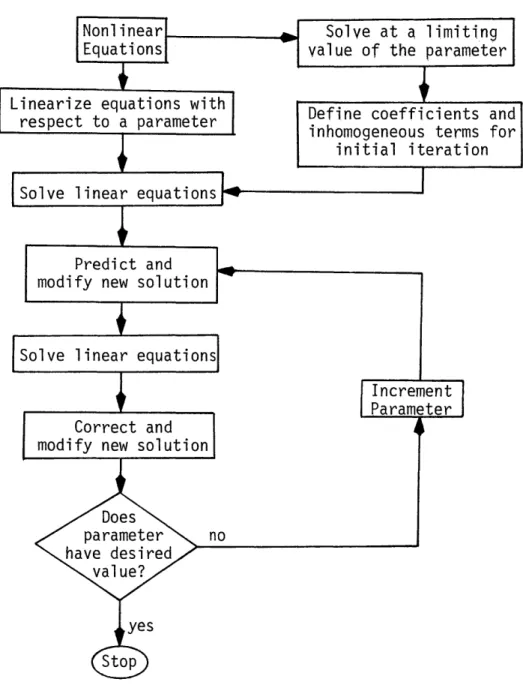
The solution process for a family of airfoils is summarized in Figure 3.1.

In order to apply the method discussed in this section, I must be able to determine the rate of change of the solution throughout the flow field. The governing equations and boundary conditions to be satisfied by are detailed in the next section.

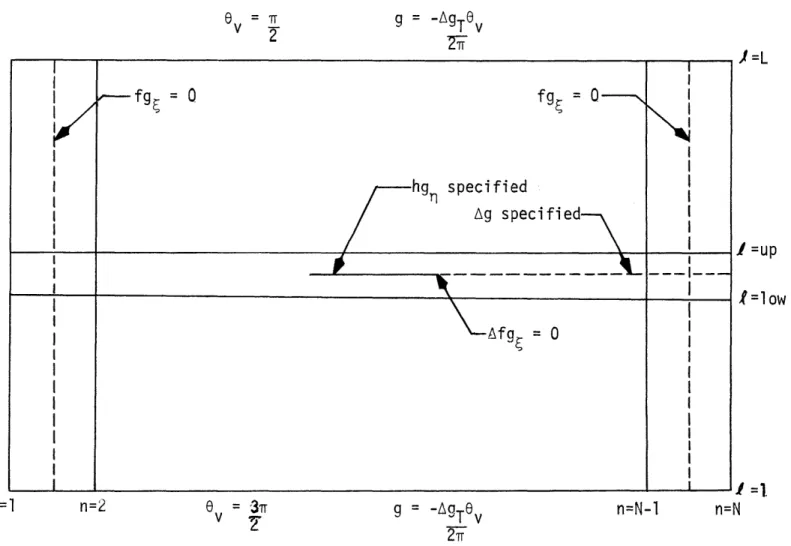
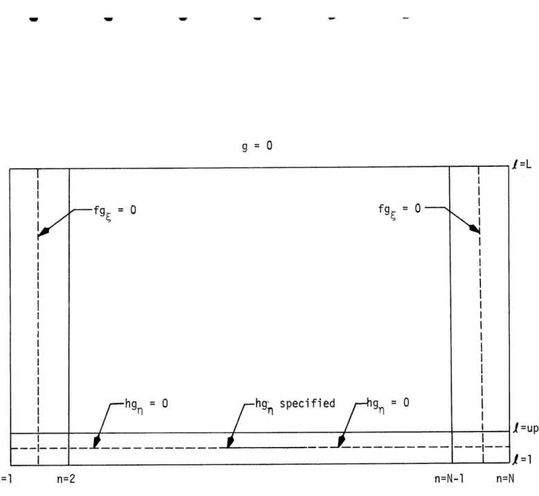
3.4. Formulation of the Linear Boundary Value Problem

Nonlinear Solve at a limiting Equations value of the parameter Linearize equations with _{Define coefficients and}

respect to a parameter j _{U mCeeouus term} P

3 U I

initial iteration Solve linear equations1

Predict and modify new solution

Solve linear equationsl

Correct and modify new solutioni

Increment Parameter Does parameter no have desired value? yes Stop

Figure 3.1. Solution procedure using the method of parametric differentiation.

I

differentiating (2.15) and (2.17)-(2.23) with respect to a character-izing parameter. The chosen parameters are the airfoil thickness ratio, Z , which characterizes nonlifting flows and the measure of camber and angle of attack, or , which characterizes lifting flows. The free stream Mach number is another possible parameter but is not used as such here.

It should be noted that neither - noro7' appears in (2.15). This is advantageous because the governing equations for both

lifting and nonlifting flows are identical and may be solved by the same numerical technique. This would not be the case if Mach number was chosen as a parameter.

Differentiating (2.15) with respect to ~Z or o , I obtain the linear equation

[i_,,,-n 2

m

An important characteristic of (3.11) is that it switches type - the quantity /-2 .. ,,4,/ changes sign - at the same points in the flow field as the nonlinear potential equation.

If the mean airfoil position is defined as

the conditions to be satisfied on the boundaries of nonlifting and lifting airfoils are, respectively

3

(3.13)

60K)

At subsonic trailing edges I require that

and along the cut in the flow field Sx= 0 IJ J X 0 Equations (3.14) (3.15) (3.16) (X -2L M

(x'c

(3.14)-(3.16) lead to the requirements that

(3.17)

downstream of subsonic trailing edges, and

(3.18)

downstream of supersonic trailing edges, where j ,. is the jump in across the trailing edge. Completing the problem specification for shockless flows is the condition that

(9- e= 0-r 0)

/1. (3.19)

When the flow becomes supercritical, additional conditions must be satisfied at any shock wave that appears in the flow field. Those conditions are easily obtained by following the technique of Murman and Cole [ 9 .

1

\ . (3.20)

The integral of (3.20) over the entire flow field is then converted to the line integral

f {-1-?M1 ri< 4+/ (3.21)

which, when integrated across a discontinuity, yields the parametric shock jump conditions

Having properly posed the linear boundary value problem, steady transonic flow solutions may be obtained. However, a base solution of the nonlinear problem is needed to initialize the solution procedure. One possibility is to solve the potential equation for a starting solution, but other realistic solutions may be easily obtained. The conditions for which those solutions

are valid are outlined below.

3.5. Formulation of Base Solutions

Miles [42 ] of (2.18) in the

and Lin, et. al. [43 ], by scaling the variables following manner

.j

f':-

Ic)

and ordering terms, have shown that the flow field is transonic if

and is subsonic or supersonic if

Since I only consider flows that are subsonic at infinity, if Z and a-are sufficiently small, the base solution will satisfy Laplace's

equation

Consequently, the base solutions may be obtained from elementary singularity distributions.

Considering the lift to be due to an angle of attack, , the starting lifting solution, # , may be obtained by distributing

a line of vortices along the airfoil chord. Extending the incompressible vorticity distribution, derived in [311, to compressible flows,

becomes

/

f

The nonlifting contribution is represented by the following distri-bution of sources and sinks along the airfoil chord

fx;-C,) =1 r'y /,A-1-> J2] el

Z'7B (3.24)

In Appendix B, (3.24) has been integrated to yield the base solution for nonlifting biconvex airfoils.

3.6. Summary

I have used the method of parametric differentiation to linearize the steady, small perturbation transonic flow problem. A predictor-corrector method for extending the solution was pre-sented, and the boundary value problem for lifting and nonlifting flows, including flows with imbedded shock waves, have been

specified. A base solution is required to initialize the solution procedure, and conditions for which relatively simple linear

base solutions may be used for this purpose are presented.

These base solutions are then represented by singularity distri-butions.

CHAPTER IV

DETERMINATION OF THE RATE OF CHANGE OF THE STEADY POTENTIAL AND RESULTS FOR STEADY FLOWS 4.1. Introduction

In order to determine the rate of change of the steady po-tentials with the chosen parameter, I must solve a linear partial differential equation with variable coefficients. Because of the variable coefficients, any solution technique that is used must be capable of admitting elliptic, hyperbolic, and discontinuous solutions. In this work, finite difference methods are applied, with appropriate difference operators being employed in the various

regions of the flow field. Those operators are constructed to allow signals to propagate in the upstream and downstream directions in subsonic (elliptic) regions and only in the downstream direction in supersonic (hyperbolic) regions.

The correct direction of signal propagation and the calcu-lation of the parametric shock jump conditions are ensured by applying the concept of conservative type dependent differencing to (3.11). This type of differencing is equivalent to adding, at all points in supersonic flow regions, an artificial viscosity of the order of the grid spacing in the streamwise direction. Derivatives in the streamwise direction are approximated with

centered differences in subsonic flow regions and with backward (upwind) differences in supersonic flow regions, and derivatives normal to the free stream are always approximated with centered differences. Where the flow accelerates through sonic velocity,

a parabolic difference operator is used, and immediately downstream of imbedded shock waves, I employ a combination of centered and backward differences.

In the numerical procedure, special measures are taken to satisfy the boundary conditions. Dirichlet conditions are satisfied by setting . along the appropriate boundary at the prescribed value, and Neumann and Robbin conditions are specified midway between grid points. Neumann and Robbin boundary con-ditions are then easily incorporated into the difference equations.

Having differenced the equation governing in the manner described above, I obtain an implicit set of simultaneous equations. Starting from the upstream boundary, I proceed downstream

cal-culating the flow field using a column relaxation method. The entire process is repeated until, throughout the flow field, the magnitude of the difference of the value of for successive

iterations and the change in j over a given number of iterations are less than predetermined constants. All compu-tations are carried out in a coordinate system that has been stretched to infinity. That stretching increases the density of

relatively fewer points in the far field.

In the remainder of this chapter, I present the numerical procedure used to solve (3.11) subject to the appropriate con-ditions; that procedure is detailed in Appendix C. Also, I present families of steady state loads on lifting and nonlifting airfoils, the convergence histories of the solutions, and some

comparisons of my data with that obtained by other researchers. 4.2. Coordinate System

At large distances from the airfoil, far field boundary conditions are to be specified, and if the computational region is extended sufficiently far, the relatively simple boundary

conditions at infinity may be utilized. Here, I use the coordinate transformation introduced by Carlson [ 44] which maps an infinite physical region into a finite computational domain and distri-butes the grid points more densely in the neighborhood of the airfoil. The infinite physical region may now be computed with a reasonable number of grid points.

The physical plane is separated into the three regions shown in Figure 4.1, and the coordinates are transformed in the following manner

I ii:

I---I I

- x₄

Figure 4.1. Regions of the physical plane.

Figure 4.2. Typical transformed coordinate system.

I III

x

4 z 5TI