Analysis of Linear Programming Relaxations for a Class of Connectivity Problems

FOR A CLASS OF

CONNECTIVITY PROBLEMS

by

MICHEL X GOEMANS

by

Michel X. Goemans

Submitted to the Sloan School of Management on August 21, 1990

in partial fulfillment of the requirements for the degree of DOCTOR OF PHILOSOPHY

IN OPERATIONS RESEARCH

Abstract

We consider the analysis of linear programming (LP) relaxations for a class of connectivity problems. The central problem in the class is the survivable network design problem -the problem of designing a minimum cost undirected network satisfying prespecified connectivity requirements between every pair of vertices. This class includes a number of classical combinatorial optimization problems as special cases such as the Steiner tree problem, the traveling salesman problem, the k-person traveling salesman problem and the k-edge-connected network problem.

We analyze a classical linear programming relaxation for this class of problems under three perspectives: structural, worst-case and probabilistic. Our analysis rests mainly upon a deep structural property, the parsimonious property, of this LP relaxation. Roughly stated, the parsimonious property says that, if the cost function satisfies the triangle inequality, there exists an optimal solution to the LP relaxation for which the degree of each vertex is the smallest it can possibly be. The numerous consequences of the parsimonious property make it particularly important.

First, several special cases of the parsimonious property are interesting properties by them-selves. For example, we derive the monotonicity of the Held-Karp lower bound for the traveling salesman problem and the fact that this bound is a relaxation on the 2-connected network problem. Another consequence is the fact that vertices with no connectivity re-quirement, such as Steiner vertices in the undirected Steiner tree problem, are unneces-sary for the LP relaxation under consideration. From the parsimonious property, it also follows that the LP relaxation bounds corresponding to the Steiner tree problem, the k-edge-connected network problem or even the Steiner k-k-edge-connected network problem can be computed a la Held and Karp.

Secondly, we use the parsimonious property to perform worst-case analyses of the duality gap corresponding to these LP relaxations. For this purpose, we introduce two heuristics

laxation of the Steiner tree problem is within twice the value of the minimum spanning tree heuristic and that several generalizations of the Steiner tree problem, including the k-edge-connected network problem, can also be approximated within a factor of 2 (in some cases, even smaller than 2). We also introduce a new relaxation a la Held and Karp for the k-person traveling salesman problem and show that a variation of an existing heuristic is within times the value of this relaxation. We show that most of our bounds are tight and we investigate whether the bound of 3 for the Held-Karp lower bound is tight.

We also perform a probabilistic analysis of the duality gap of these LP relaxations. The model we consider is the Euclidean model. We generalize Steele's theorem on the asymp-totic behavior of Euclidean functionals in a way that is particularly convenient for the analysis of LP relaxations. We show that, under the Euclidean model, the duality gap is almost surely a constant and we provide theoretical and empirical bounds on these constants for different problems. From this analysis, we conclude that the undirected LP relaxation for the Steiner tree problem is fairly loose.

Finally, we consider the use of directed relaxations for undirected problems. We establish in which settings a related parsimonious property holds and show that, for the Steiner tree problem, the directed relaxation strictly improves upon the undirected relaxation in the worst-case. This latter result uses an elementary but powerful property of linear programs.

I would like to express my thanks to the members of my committee, Dimitris Bertsimas, Tom Magnanti and Jim Orlin, for their encouragement and support. Through them, I was exposed to the many facets of academia.

I am also grateful to Laurence Wolsey for sharing thoughts on the worst-case analysis of linear programming relaxations, David Shmoys and David Williamson for stimulating some of this work, Dan Bienstock for challenging me on the simplicity of certain proofs, David Johnson for hosting me at AT&T Bell Labs during the summer 1989 and all my chess partners for their master strokes.

I would like to thank all my friends at the OR Center, past and present, for giving this place such a warm atmosphere. I especially wish to thank Murali for his fascinating stories, Leslie for her enthusiasm, Kalyan for numerous stimulating discussions, Philippe for letting me baby-sit Jonathan, Ski for coining the term "mildly Hamiltonian", Andrew for his humour, Mostafa for his relaxed attitude, Octavio for reviving my passion for sailing and many more for proofreading these acknowledgements.

It is hard to adequately express my gratitude and thanks to my wife Catherine for her love, caring and faith in my abilities. She was always present even when, with my unblinking gaze and a hand under the chin, I was deeply lost in my research thoughts.

This research was supported in part by the Belgian American Educational Founda-tion and by the NaFounda-tional Science FoundaFounda-tion under grants #ECS-8717970 and #DDM-9010322.

Abstract .

Acknowledgements 1 Introduction

1.1 The Survivable Network Design Problem ... 1.1.1 Formulations.

1.1.2 Algorithms.

1.2 The Traveling Salesman Problem ... 1.2.1 Relaxations ...

1.3 The k-Person Traveling Salesman Problem .

2 Structural Properties

2.1 The Parsimonious Property ... 2.2 Extensions . ... 2.3 Monotonicity ...

3 Special Cases and Algorithmic Consequences

3.1 Elaboration on a Lagrangean approach for General

1 5 9 ... 10 ... 10 ... 16

23

. . . 23

4.2 The Tree Heuristic ...

4.2.1 The Steiner Tree Problem ... 4.2.2 The General Case ... 4.3 The Improved Tree Heuristic ...

4.3.1 The Traveling Salesman Problem . . . 4.3.2 The General Case ...

4.4 The k-Person Traveling Salesman Problem. 4.5 Tightness of the Bounds.

4.5.1 The Tree Heuristic ...

4.5.2 The Held-Karp Lower Bound ...

53 53 57 58 61 65 67 68 70 73 73 80 v i iii. loll ... ... ... ... ... ... ... ... ... ... ...

5 Probabilistic Analysis 87

5.1 Euclidean Model and Literature Review . ... 87

5.2 Asymptotic Behavior of Euclidean Functionals . ... 89

5.2.1 Review of Stochastic Convergence ... 89

5.2.2 Steele's Theorem ... ... 89

5.2.3 A Generalization ... 92

5.2.4 Some Illustrations .. ... 1... 102

5.3 The Held-Karp Lower Bound . ... 107

5.3.1 The Uniform Case ... 107

5.3.2 The Non-Uniform Case . . . ... 113

5.3.3 Bounds on the Constants P's ... 116

5.4 The Survivable Network Design Problem . ... 119

5.5 Partitioning Schemes ... 122

6 Directed versus Undirected Formulations 125 6.1 The Parsimonious Property ... 128

6.2 The Steiner Tree Problem ... 130

6.2.1 Worst-Case Analysis ... 131

6.2.2 Probabilistic Analysis ... 133

7 Short Summary and Open Problems 135

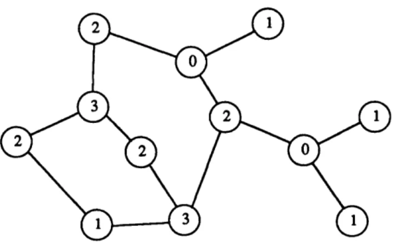
1.1 A survivable network: the connectivity types are indicated inside each vertex. 4

1.2 A 2+2-tree ... 17

2.1 Graph G ... 27

2.2 1-tree in A. .. ... ... 35

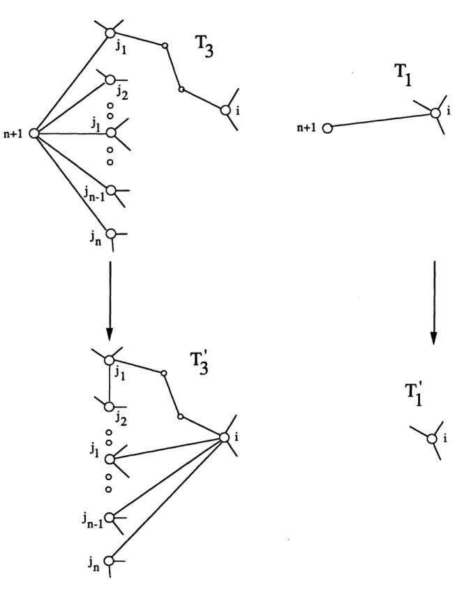
2.3 Construction of T and T. ... ... 38

3.1 Counterexample for gl(A): The connectivity types are indicated inside each vertex ... . 50

3.2 Counterexample for g2(A): The connectivity types are indicated inside each vertex ... . 50

3.3 Counterexample for g3(A): The connectivity types are indicated inside each vertex ... . 51

4.1 Example in the proof of Theorem 4.3. ... 63

4.2 Worst-case instance for the tree heuristic for the Steiner tree problem. .... 74

4.3 Worst-case instance for the undirected LP relaxation for the Steiner tree problem . ... ... 74

4.4 How to generate k-connected k-regular graphs. ... 76

4.5 Graph G1for L = {1,2,3} and q = 4. ... 77

4.6 Worst-case instance for ... . 82

5.1 A possible numbering of the subsquares when d = 2. . ... 103

5.2 Step 1 in the construction of TA ... 110

5.3 Step 2 in the construction of TA ... 112

6.1 A counterexample to the directed parsimonious property. ... 129

4.1 A few special cases of Theorem 4.2 ... 63 4.2 A few special cases of Theorem 4.3. . . . 65 4.3 A few special cases of Theorems 4.2, 4.3, 4.7 and 4.9 ... 71

Introduction

In recent years, linear programming has emerged as a powerful tool in order to tackle NP-hard combinatorial optimization problems.

The first important application of linear programming (LP) relaxations is in design-ing branch-and-bound or branch-and-cut algorithms to solve combinatorial optimization problems to optimality. For a general exposition to branch-and-bound schemes, we refer the reader to the books by Nemhauser and Wolsey [86] and Minoux [80]. In general, the closer the LP relaxation value is to the integer programming value the better the perfor-mance of these schemes is. In addition, by solving the linear programming relaxation of certain problems (or its dual) and using heuristic methods to obtain good feasible solu-tions, researchers have been able to solve other large scale applications to near optimality, with performance guarantees concerning the degree of suboptimality. For example, re-searchers have solved network design models with up to 500 design arcs, 2 million flow variables and 2 million constraints to within 1-2% of optimality (Balakrishnan, Magnanti and Wong [3]), traveling salesman problems with up to 100,000 nodes to within 1% of optimality (Johnson [61,62]), as well as large scale Steiner tree problems (Wong [112]) and facility location problems (Cornuejols, Fisher and Nemhauser [20]).

Another important area where LP relaxations can play a very significant role is to assess a priori the quality of a heuristic for a hard combinatorial optimization problem. Indeed, worst-case analyses typically rely on comparing the value of the heuristic solution

to some lower bound for the problem, often obtained through the apparatus of linear pro-gramming (Wolsey [111]). This allows one to claim that the heuristic is always within a certain percentage of the unknown optimal solution. Moreover, LP relaxations sometimes intervene not only in the analysis of heuristics but also in their design. Heuristics based on rounding linear programming solutions were proposed for scheduling unrelated parallel machines (Lenstra, Shmoys and Tardos [73]), for the prize-collecting traveling salesman problem (Bienstock, Goemans, Simchi-Levi and Williamson [10]) and for some multicom-modity flow problem (Raghavan and Thompson [93]). These heuristics have interesting worst-case guarantees in the former two cases and probabilistic guarantees in the latter case.

The above discussion stresses the importance of obtaining efficiently strong LP relax-ation bounds, analyzing their performance and relating them to heuristic algorithms. In this thesis, we study from several perspectives the LP relaxations of a class of network design problems in which connectivity constraints play a priviledged role. This class in-cludes a number of classical combinatorial optimization problems as special cases such as the Steiner tree problem, the traveling salesman problem, the k-person traveling salesman problem and the k-edge-connected network problem. The central problem in the class is, however, the survivable network design problem - the problem of designing, at minimum cost, a network satisfying certain survivability constraints.

In the rest of this chapter, we describe the combinatorial optimization problems, their formulations and the relaxations that are the focus of this dissertation. Among the re-laxations presented, we would like to mention a new relaxation for the k-person traveling salesman problem. In Chapter 2, we present and prove the parsimonious property - a very important structural property of a class of LP relaxations for the survivable network design problem. We also investigate for which linear programs a similar property holds, and we present a closely related property of these relaxations, namely their monotonic-ity. Chapter 3 focuses on the algorithmic implications of the parsimonious property. In Chapter 4, we introduce some heuristics for the problems under investigation and relate their values to the LP relaxation bounds and to the optimal values, therefore performing

worst-case analyses. We also examine whether these proposed worst-case bounds are tight. To explain the behavior of LP relaxations on typical instances, we perform a probabilistic analysis of these LP relaxations under the Euclidean model in Chapter 5. For that pur-pose, we prove a general result on the asymptotic behavior of linear or integer programs satisfying some fairly mild assumptions. Finally, in Chapter 6, we consider the use of di-rected formulations for combinatorial problems defined on undidi-rected graphs. We examine whether the parsimonious property holds for directed formulations and we compare the

LP relaxations of undirected and directed formulations for the Steiner tree problem.

1.1

The Survivable Network Design Problem

Networks arising in transportation or communication systems often need a certain level of survivability. Informally, survivability is the ability to reroute the traffic through alternate paths after the failure or loss of one or several links. More formally, we associate to vertex

i a connectivity type ri representing the importance of communication from and to vertex i and we call an undirected network survivable if it has at least rij = min(ri, rj)

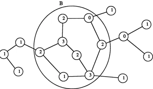
edge-disjoint paths between any pair of vertices i and j. More generally, we do not necessarily assume that the connectivity requirements rij are of the form min(ri, rj) for some vector r. In a survivable network, the loss or failure of any k edges still allows communication between pairs of vertices whose connectivity requirement is greater than k. By abuse of notation, we use r to denote both the matrix r = [rij] of connectivity requirements and, if applicable, the vector r = [ri] of connectivity types. An example of a survivable network is given in Figure 1.1.

Gomory and Hu [47] show that the analysis problem of checking whether a given network is survivable can be solved by means of n maximum flow problems, where n, throughout this thesis, represents the number of vertices in the network. Given a complete undirected network G = (V, E), a cost cij associated with each edge' (i,j) E E and an integral symmetric matrix r = [rij] of connectivity requirements, we consider, in this 'For undirected networks or graphs, we implicitly assume that both (i, j) and (j, i) represent the same edge.

Figure 1.1: A survivable network: the connectivity types are indicated inside each vertex.

thesis, the problem of selecting a subset of the edges (repetition is allowed) so that the resulting network is survivable and its total cost is minimum over all such networks. This problem is referred to as the survivable network design problem (SNDP). It is also known as the multiterminal synthesis problem [47,38] or the generalized Steiner problem [110].

The survivable network design problem is of particular importance in the design of communication or transportation systems in which the lack of communication or connec-tivity between parts of the network might be catastrophic. For example, this issue is particularly relevant in the design of communication systems using fiber optic links (see Monma et al. [83,81], Cardwell et al. [11] or Gr6tschel et al. [53]). Indeed, these links have extremely high capacity and, thus, the network planner might be tempted to design tree-like topologies in order to minimize the design costs. However, in these topologies, the loss of a single link disrupts communication between parts of the network. Moreover, losses of this type are not atypical (see [81,53]). The network designer must therefore make tradeoffs between the total design cost and the capability of the network to restore service in case of failures. In this context, the survivable network design problem we have just described constitutes an adequate model for these tradeoffs. A slightly different model, allowing vertex connectivity requirements and forbidding multiple links, is being used by practitioners from Bellcore (see [11]).

The SNDP has some interesting special cases. The undirected Steiner tree problem consists in finding a minimum cost tree of an undirected network G = (V, E) spanning a prespecified subset T of compulsory vertices, also called terminals, and possibly using some optional vertices, also called Steiner vertices. This problem can be modeled as an SNDP by letting the connectivity types ri to be 1 for the set T of terminals, and 0 for the Steiner vertices. Consequently, the minimum spanning tree (T = V) and the shortest path problem (ITt = 2) are also special cases. When the requirements are uniform, say equal to k, the SNDP reduces to the k-edge-connected network problem - the problem of designing a minimum cost k-edge-connected network. A closely related problem is the k-connected network problem in which the network is required to have k vertex-disjoint paths between every pair of vertices. Under the triangle inequality, the 2-edge-connected network problem and the 2-connected network problem are equivalent (see [41]), but, in general, the edge and vertex versions are different.

1.1.1 Formulations

The survivable network design problem can be formulated as an integer program in two equivalent ways. The first formulation is a multi-commodity based formulation:

Minimize

E

ceXe

eEE

subject to:

rij

i < j and k = i

(SNDPY) = i < j and k E V \ {i,j}

IEV IEV

-rij i < j and k = j

0 < Yk < xe e =

(k,

or (, k) and i < j

Xe integral e E E.

In this formulation, zx (e E E) denotes the number of times edge e is selected in the solution and Ykl represents the amount of flow along the directed arc (k, I) corresponding

to the commodity whose origin is vertex i and destination vertex j. The validity of this formulation follows from the fact that the flow variables y can be chosen to be integral and

therefore the network corresponding to any feasible solution has at least rij edge-disjoint paths between any pair (i,j) of vertices. By projecting the feasible space of (SNDP1)

onto the z variables, we obtain the following equivalent formulation:

Minimize

E

CeXe

E

0

<

where 6(S) represents the set of edges connecting S to V \ S. To see that the feasible space of (SNDP2) is the projection of the feasible space of (SNDP1), consider a feasible

solution z to (SNDP2). Since constraints (1.1) insure that the value of a minimum cut

separating i from j is at least rij, it is possible to send rij units of flow from i to j by the max-flow-min-cut theorem [35]. This means that there exists y such that (x,y) is feasible in (SNDP1). Conversely, if (,y) is feasible in (SNDP1), all constraints (1.1)

must be satisfied and, hence, x is feasible in (SNDP2). Let (P1) and (P2) denote the

linear programming (LP) relaxations of (SNDP1) and (SNDP2) obtained by dropping

the integrality restrictions. Using the same argument, (P1) and (P2) are equivalent. More

precisely, the feasible space of (P2) is exactly the projection of the feasible space of (P1)

onto the space defined by the z variables. In other words, (P1) constitutes a compact extended formulation of the natural formulation (P2). The optimal value of (P1) or (P2)

can be computed in polynomial time either using the ellipsoid algorithm [69,49] since the separation problem over (P2) can be solved by Gomory and Hu's algorithm [47] or using

Karmarkar's algorithm [65] on the compact (but still large) linear program (P1). However,

these computational approaches are not satisfactory in practice and, in fact, one of the goals of this research is to obtain a better understanding of the structure of these LP relaxations in order to be able to devise more efficient and practical algorithms.

and, therefore, formulation (SNDP2) becomes:

Minimize

E

eEE

subject to:

(UST)

E

1

SC V,SnTlOand T\Si0

CEa(S)

O

e

E

ze integral e E E.

Formulation (UST) is known as the set covering formulation for the undirected Steiner tree problem (Aneja [1]). There also exists a directed counterpart to the undirected Steiner tree problem. In this case, we are given a directed network with costs associated to its arcs and the goal is to find, at minimum cost, a directed subtree that contains a directed path between some given root verter, say vertex 1 (1 E T), and every other terminal in T. Since, for any choice of root vertex, any undirected tree can be oriented away from that root, the undirected version is a special case of the directed version. More precisely, the undirected Steiner tree problem is equivalent to the bi-directed problem, i.e. the directed version with symmetric costs (cij = cji). However, both problems are worth investigating and the reduction between the undirected and the bi-directed cases will be used in a subsequent chapter to obtain properties of Steiner tree relaxations. For the directed (or bi-directed) Steiner tree problem, the analogue of formulation (UST) is:

Minimize

E

(DST)

Yij

1

S C V, l E S and T\S

Yij integral (i,j) E A,

where 6+(S) represents the set of arcs (i,j) with tail i E S and head j S, and where Ye is defined for each (directed) arc e. Although the integer program (UST) and its bi-directed counterpart (DST) are equivalent, this is not the case for their LP relaxations

obtained by dropping the integrality constraints. Let (DP) and (UP) represent the linear programming relaxations of (DST) and (UST) respectively. Since any feasible solution y to (DP) can be transformed into a feasible solution z to (UP) by letting zx = yij + yji for e = (i, j), the optimal value of (DP) is greater or equal to the optimal value of (UP).

However, the converse is not true.

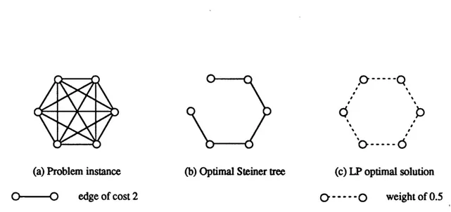
For some special cases, the Steiner tree problem reduces to well-known, polynomial time solvable, combinatorial optimization problems. When ITI = 2, we obtain the shortest path problem. Both (UP) and (DP) are integral2 _{for that very special case (Dantzig [24]).}

When T = V, the problem becomes the minimum spanning tree in the undirected case and the minimum cost spanning arborescence in the directed case. A very peculiar property is that, in this case, (DP) is integral (Edmonds [27]) while (UP) is not. To see that the extreme points of (UP) are not necessarily incidence vectors of spanning trees, consider a minimum spanning tree problem with 3 vertices and all costs equal to 1. The minimum spanning tree has cost 2 while, by setting all variables xz to 0.5, we obtain a feasible solution to (UP) of cost 1.5. In subsequent chapters, we study this phenomenon in more details.

Recently, there has been a trend towards finding strong valid inequalities of combinato-rial optimization polytopes in order to tighten the LP relaxations of existing formulations. By generating violated valid inequalities on the fly, researchers have been able to solve some fairly large problems to optimality (for illustrations, see Crowder and Padberg [23], Padberg and Rinaldi [88], Crowder, Johnson and Padberg [22] or Barany, Van Roy and Wolsey [6]). Gr6tschel and Monma [50] and Gr6tschel, Monma and Stoer [51,53] have developed classes of valid inequalities for the SNDP (allowing vertex-connectivity require-ments). In [53], the authors focus their attention on the case where ri E {0, 1, 2}. More-over, Gr6tschel, Monma and Stoer [52,53] have implemented a cutting plane algorithm based on these classes of strong valid inequalities and have reported some encouraging computational results.

For the Steiner tree problem, Liu [74] uses a complete characterization of the directed

2

Steiner tree polytope when ITI = 3 to motivate a reformulation for the problem. Moreover, Chopra and Rao [15] and Gr6tschel and Monma [50] have studied some classes of facets for the Steiner tree polytope.

1.1.2 Algorithms

When all edges have a unit cost, the survivable network design problem can be solved in polynomial time by an algorithm due to Sridhar and Chandrasekaran [99] (see also Frank [37]) - an adaptation of the classical Gomory and Hu's algorithm [47] producing a network with possibly half edges. For arbitrary costs, the SNDP, generalizing the Steiner tree problem and the 2-connected network problem, is NP-hard [66]. Typically, such a negative result from complexity theory leads researchers to obtain approximate rather than optimal solutions and to devise lower bounding schemes. In fact, heuristic algorithms based on local search have been proposed by Steiglitz et al. [105] for the SNDP in its full generality, by Monma and Ko [81] for the k-edge-connected network problem (ri = k for all i) and by Monma and Shallcross [83] for the case where ri E {1,2) for all i.

For the Steiner tree problem, a wide variety of computational approaches have been proposed (for a survey, see Winter [110] or Maculan [77]). Two of these approaches are of special interest to us since they are based on solving linear programming relaxations. Aneja [1] solves the relaxation (UP) by row generation and heuristically deduces from this solution a good Steiner tree. Wong [112] proposes a dual ascent method to solve approx-imately (DP) or, more precisely, its equivalent multi-commodity relaxation. Aneja's and Wong's computational results seem to show that both procedures are very efficient. Aneja and Wong notice that the LP bounds obtained are very close to the value of the optimal Steiner tree. However, in Chapters 4 and 6, we present some evidence that, for undirected instances, the undirected relaxation (UP) is sometimes much weaker than the bi-directed relaxation (DP). We therefore believe that Aneja's test problems do not reflect the real behavior of the relaxation (UP).

1.2

The Traveling Salesman Problem

As we'll see when presenting the parsimonious property, it is very natural to consider a broader class of problems in which we allow the addition of degree constraints to the problem formulation. This extended version captures the well celebrated symmetric trav-eling salesman problem (TSP) - one of the most studied problem in the literature (see Lawler et al. [72]). This problem can be defined as follows: given a cost c, associated with traveling along the edge e of the complete undirected graph G = (V, E), find the minimum cost tour that visits each vertex exactly once. It is conceptually useful to define a tour as a subgraph that is connected and such that every node has degree 2. Several integer programming formulations have been proposed for the TSP. Letting xe = 1 (e = (i,j)) if

i and j are adjacent vertices in the optimal tour, one of the most classical formulation for the TSP is: Minimize g CetX eEE subject to:

(TSP)

Z

xe

2

SCV and IS

>

2

E

=2

1.2.1

Relaxations

Since the traveling salesman problem is NP-hard [66], a number of branch and bound methods have been devised (see Balas and Toth [5]). An important ingredient in these enumerative methods is the relaxation used to obtain lower bounds in the bounding step. The integer 2-matching relaxation, also called the assignment relaxation (especially when dealing with the asymmetric TSP), consists in finding the minimum cost assignment of weights 0, 1 or 2 to the edges of the graph G so that the sum of the weights on the edges incident to any vertex is 2. The integer 2-matching relaxation can be reduced to an n by

n assignment problem and, therefore, can be computed in polynomial time. If we restrict

the weights to {0, 1), the edges with weight 1 form what is called a 2-matching, that is a collection of vertex-disjoint subtours. The 2-matching relaxation was introduced by Bellmore and Malone [8] and its bound can be computed in polynomial time (Edmonds [25]). These first 2 relaxations do not take into account the connectedness of a tour. On the other hand, by imposing only that the subgraph be connected, we obtain the minimum spanning tree problem which can be solved in polynomial time using the greedy algorithm (Kruskal [71]) or Prim's algorithm [92]. A slightly better relaxation can be obtained by considering 1-trees.

Definition 1.1 T = (V, B) is a 1-tree (rooted at vertex 1) if T consists of a spanning tree

on V \ {1}, together with two edges incident to vertez 1.

Equivalently,

Definition 1.2 T = (V, B) is a 1-tree if

1. T is connected

2.

IVI

=

IBI

3. T has a cycle containing vertex 1 4. the degree in T of vertex 1 is 2.

Clearly, any tour is a 1-tree. The 1-tree relaxation (Held and Karp [55]) consists in finding the minimum cost 1-tree. The minimum cost 1-tree can be obtained by computing the minimum spanning tree on V \ {1} and adding the two least cost edges incident to vertex

1.

A more elaborate and much stronger relaxation, also due to Held and Karp [55,56], is now known as the Held-Karp lower bound. This relaxation constitutes the core of this dissertation. The Held-Karp lower bound ZHK can be formulated in several equivalent ways, the most classical being in terms of the 1-tree relaxation with Lagrangean objective

function [55,56]. As a linear program [55], it can be expressed as the optimal value of the LP relaxation of formulation (TSP) for the TSP:

ZHK = Min ECeXe eEE subject to: (HK1) z > 2 S C V and 151

>

Ze=2

i EV

(1.3)

The feasible space of (HK1) is sometimes referred to as the subtour polytope. Notice that the constraints xe < 1 are implied by (1.2) and (1.3). Indeed, for e = (i,j),

2xe=

E

E

E

fe6({i}) fEs({j}) fE6({i,j})

By adding up constraints (1.3) over all i in S, we obtain:

2

E

x +

Z

xc = 21SI,

(1.4)

eEE(S) eE6(S)

where E(S) denotes the set of edges having both endpoints in S. Using equation (1.4), the subtour elimination constraints (1.2) are equivalent to:

E

e 1Xe•

-1,

(1.5)

eEE(S)

for all proper subsets S of V of cardinality at least 2. Hence, the Held-Karp lower bound can also be expressed by:

ZHK = Min E ceX eEE subject to: (HK2)

E

Xc

<

E

X = 2

i

E

V

(1.7)

Held and Karp [55] highlight the relation between the linear programs (HK1) and (HK2)

and the class of 1-trees. More precisely, they show that the feasible solutions to (HK1)

or (HK2) can be equivalently characterized as convex combinations of 1-trees such that

each vertex has degree 2 on the average. To show this, we first notice that we can restrict our attention in (1.6) to subsets S not containing vertex 1. Indeed,

1 1

Z re =

z

t

E

2

E

eEE(S) eEE(V\S) iEs eE6({i}) ifs eE6({i})

=

E

X

+ 2SI-n,

eEE(V\S)

which implies that both V \ S and S need not be included in the formulation. Therefore, the Held-Karp lower bound can be expressed by:

ZHK =

Min

E

CeX

E

iE

V

i1

(1.8)

> 2

1

E

E

<

constraint (1.10) being obtained by summing up constraints (1.7) for all i except vertex 1 and then substracting constraint (1.7) for vertex 1. Since constraints (1.9), (1.10) and (1.12) constitute a complete description of the spanning tree polytope on V \ 1} (Ed-monds [28,29]) and since constraints (1.11) and (1.12) correspond to the convex hull of the incidence vector of two edges incident to vertex 1, the polytope (1.9)-(1.12) completely describes the convex hull of 1-trees [55]. As a result, the feasible solutions to (HK1),

(HK2) or (HK3) can be interpreted as convex combinations of 1-trees such that each

the following way [55]: k ZHK = Min

E

(HK

)

= 1

Ard(Tr)=2

j

V\{1}

{Tr)}r=l

constitutes the class of 1-trees defined on the vertex set V,

*

c(T) =

cC is the total cost of the subgraph T = (V, B) and

eEB

*

dj(T) denotes the degree in T of vertex j.

Finally, the most common approach to find the Held-Karp lower bound is to take the

Lagrangean dual of (HK

) with respect to (1.8). We then obtain [55]:

ZHK = max L(p)

subject to:

(HK

)

L() =

C,(Tr)- 2

where c (Tr) is the cost of the 1-tree Tr with respect to the costs c, + pi + Pj for e = (i, j).

The j's are known as Lagrangean multipliers.

Since (HK

) is the most classical formulation for the bound, the Held-Karp lower

bound is often referred to as the 1-tree relaxation with Lagrangean objective function.

We would like to mention that Held and Karp's papers [55,56] really constitute the birth

of the Lagrangean relaxation approach for combinatorial optimization problems as it exists

nowadays.

For fixed , L(p) can be computed by finding the minimum cost 1-tree and,

there-fore, the Lagrangean subproblems can be solved efficiently. In order to find a good set

of Lagrangean multipliers, several updating procedures have been proposed. The most used and well-known procedure is the subgradient method introduced by Held and Karp [56]. The method is an adaption of steepest descent in which gradients are replaced by subgradients. We refer the reader to Held, Wolfe and Crowder [57] and their refer-ences for a detailed exposition and analysis of subgradient optimization. If T is a min-imum cost 1-tree with respect to the costs {c,}, the optimality conditions imply that v = (dl(T) - 2, d2(T)- 2,...

,dn(T)-

propose the following updating formula for the Lagrangean multipliers:

m+1 = Am + tmVr,

where vm is a subgradient of L(pm) and tm is a scalar. In their computations, they set tm = t for all m. They prove that, as the step size t becomes infinitesimally small, supm L(pm) tends to max, L(p). In their first paper [55], Held and Karp proposed a rather unsuccessful procedure based on dual ascent to compute max, L(p). This seemed to discourage other researchers for some time, but very recently, Malik and Fisher [79] reported very encouraging computational results based on a more complex ascent proce-dure. Their method seems to outperform the subgradient method in early and middle stages of ascent but is slower in the neighborhood of the optimum. Finally, Chandru and Trick [12] propose a polynomial time algorithm to find the optimum multipliers using the ellipsoid algorithm but they report computational times that are two to three times slower than the subgradient method.

In a striking computational study, D. Johnson [61,621 estimates the degree of subopti-mality of heuristic solutions by computing approximately the Held-Karp lower bound and, as a result, he is able to show that the solutions he generates are within 1% of optimality for instances with as many as 100,000 vertices. Earlier computational studies on smaller instances also corroborate the fact that the Held-Karp lower bound is often within 1% of the optimal solution (Christofides [17] and Volgenant and Jonker [108]). Moreover, the Held-Karp lower bound has been successfully used by several researchers (Held and Karp [56], Helbig Hansen and Krarup [54], Smith and Thompson [98] and Volgenant and Jonker [108]) to solve exactly instances of the TSP by branch-and-bound methods. For a detailed

exposition of branch-and-bound schemes for the traveling salesman problem, the reader is referred to Balas and Toth [5].

We would like to close this section by mentioning that numerous heuristics have been devised for the traveling salesman problem (see Johnson and Papadimitriou [63] and also Chapter 4) and that, in the last decade, polyhedral approaches have proven very successful for medium sized instances (see Crowder and Padberg [23], Padberg and Rinaldi [88] and Padberg and Gr6tschel [87]).

1.3

The k-Person Traveling Salesman Problem

As a direct extension to the traveling salesman problem, we consider the problem in which there are k salesmen to visit all customers. A k-tour is a collection of k cycles starting at vertex 1 and collectively visiting every vertex. The k-person traveling salesman problem (k-person TSP) is the problem of finding a k-tour of minimum length or cost. We would like to emphasize that, as in Frieze [42], the objective we consider is to minimize the total length of all cycles. This is in contrast with the original version introduced by Frederickson et al. [40] (see also Johnson and Papadimitriou [63]) in which the objective is to minimize the length of the longest cycle in the solution.

The k-person traveling salesman problem can be formulated as an integer program in a way very similar to the formulation (TSP) of the traveling salesman problem.

Minimize

E

- TSP)

Z:

=2k

ze

= 2

i

V

where V' = V \ {1}. In this case, the constraints xe < 1 are not redundant for e E 6({1}). Very little work has been done on the k-person traveling salesman problem. Moti-vated by Held and Karp's approach for the traveling salesman problem, we propose two relaxations for the k-person traveling salesman problem. In our relaxations, the role of the 1-trees is played by what we refer to as k+k-tree.

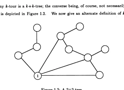
Definition 1.3 A k+k-tree T is a spanning tree with k edges incident to vertex 1 along

with k additional edges incident to vertex 1.

Equivalently,

Definition 1.4 T = (V, B) is a k+k-tree if

1. T is a connected graph,

2. the degree in T of vertex 1 is 2k, and

3. when restricted to E(V \ {1}), T becomes a forest with exactly k components.

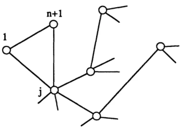
Clearly, any k-tour is a k+k-tree; the converse being, of course, not necessarily true. A k+k-tree is depicted in Figure 1.2. We now give an alternate definition of k+k-trees

Figure 1.2: A 2+2-tree.

using matroid theory. From this definition, we shall derive a complete characterization of the convex hull of k+k-trees and a polynomial time procedure to find minimum weight k + k-trees.

Definition 1.5 T = (V,B) is a k+k-tree if B is a common base of the matroids M1 =

(E,I1) and M2 = (E,Z2) where

* A E ix if the graph (V,A) has degree at most 2k at vertex 1 and the restriction of (V, A) to V' = V \ {1} is acyclic and has at most n - k - 1 edges,

* A E .l2 if A arises from some forest by adding at most k edges.

M1 is a matroid since it is the direct sum of a truncated graphic matroid (on V') and

a generalized partition matroid (restricting the degree of vertex 1 to be at most 2k). In order to show that M2 is also a matroid, let A' be a maximal independent subset of a set

A of edges with respect to M2. The set A' has exactly the same connected components as A (otherwise, we could add some edges) and, hence, consists of a forest with n - c(V, A)

edges, where c(G) denotes the number of connected components of G, together with either a set of k edges or the remaining edges whichever is smaller. Since all maximal independent subsets of a given set A of edges have the same cardinality, M2 is a matroid. The rank

functions rl and r2 of M1 and M2 are:

rl(A) = min(2k, jA

n

6({1})I) +

min(n

1

c(V', E(V') n A), n

k

1)

r2(A) = min(lAl, n + k - c(V, A)).

Claim 1.1 Definitions 1.4 and 1.5 are equivalent.

It is easy to see that any k+k-tree as defined in Definition 1.4 satisfies the conditions of Definition 1.5. To show the converse, let B be any common base of M1 and M2. Since B is a base of M, B has degree 2k at vertex 1,

lBI = n + k - 1 and the restriction of B to E(V') is a forest with n - k - 1

edges and, hence, this forest has exactly k components. The fact that B is a base of M2 and JlB = n + k - 1 implies that B arises from a spanning tree

by adding k edges. Hence, (V, B) is a connected graph. This proves that B

The first relaxation we consider is the k + k-tree relazation obtained by finding the minimum cost k+k-tree. Since this problem can be interpreted as the problem of finding a minimum weight common base of the intersection of two matroids, it can be solved in polynomial time (Edmonds [28,30]). Moreover, by Edmonds' intersection theorem [28,30], we can express the value Zkt of the k+k-tree relaxation by:

Zkt = Min _{E CeXe} eEE subject to:

E

Xc,<•Sl1

E

Xe<ISl+k-1

Z

:Z

2k

0

<x,

< 1

V'

ISI

2

since the convex hull of k+k-trees is completely described by the above feasible space. In this description, we have eliminated some of the redundant constraints.

In order to propose a stronger relaxation to the k-person traveling salesman problem, we introduce in (k + k - tree) the additional degree constraints

E Xe=2

eE6({i})

for i E V'. As for the Held-Karp lower bound, the resulting relaxation can be formulated in several equivalent ways. First, it can be expressed by the linear program:

Zklp = Min

E

E

Xe

<

S-1

(PI)

z

S

V' and

ISI

2

xe,=n-k-1 (1.16) eEE(V')

E

Ze = 2k

(1.17)

O

In this formulation, the constraints (1.15) and (1.16) are redundant since they are both implied by (1.17) and (1.18). Moreover, using (1.18), constraints (1.14) can be equivalently written as:

E

>

eE6(S)

Therefore, Zklp is also equal to:

Zklp = Min

E

Z

Xe

ISI > 2

Z

e <1

(P2) is precisely the linear programming relaxation of the formulation (k - TSP) of the

k-person traveling salesman problem. As for the Held-Karp lower bound, Zklp can also be expressed by: Zklp = Min A,c(T,) r=1 subject to: (P3) ZAr=1 r=1 E dj(Tr)=

2

where

* {Tr}=l ... constitutes the class of k+k-trees defined on the vertex set V,

*

eEB

* dj(T) denotes the degree in T of vertex j.

Finally, as a Lagrangean dual, Zklp can be expressed by:

Zklp = max L(p)

subject to:

(P₄) L(p) = min c,(Tr)-2

j

r=1...1

_jEv

where c,(Tr) is the cost of the k+k-tree Tr with respect to the costs ce + Hi + -j for

e = (i,j) ( =

0)-In terms of actually computing the lower bound Zklp, this Lagrangean based relaxation seems very promising. However, implementation issues such as how to apply the matroid intersection algorithm to k+k-trees and how to update the Lagrangean multipliers need first to be considered.

Structural Properties

In Section 2.1, we introduce the notion of parsimonious solutions, and we present and prove the parsimonious property for a class of linear programs which includes the LP relaxations of the survivable network design problem and the traveling salesman problem. Extensions to other classes of linear programs are considered in Section 2.2. We conclude this chapter by deducing the monotonicity of certain linear programs from the parsimonious property and we give an alternate proof of this property for the Held-Karp lower bound.

2.1

The Parsimonious Property

As seen in Chapter 1, the survivable network design problem can be formulated by the following integer program:

IZO(r) = Min E ce

eEE

subject to:

(IPO(r))

E

max rij

S C V and S

0

(2.1)

eE(S) (ij)Es(s)

O < xe e E

Xe integral e E E.

We denote by (IPO(r)) the above integer program and by IZO(r) its optimal value. Let

(PO(r)) denote the LP relaxation of (IPO(r)) obtained by dropping the integrality

tions and let Zo(r) be its optimal value. Clearly Zo(r) is a lower bound on IZO(r). The meaning of the symbol 0 in this notation will become clear shortly.

As noticed in Chapter 1, the survivable network design problem has some interesting special cases. For example, the Steiner tree problem - the problem of connecting at minimum cost a subset T of terminals possibly using some Steiner vertices in V \ T - can be formulated as (IPO(IT)) where (IT)ij = 1 if i,j E T and 0 otherwise (or, equivalently

using our abuse of notation, (T)i = 1 if i E T and 0 otherwise). When rij = k for all

i,j E V, we obtain the k-edge-connected network problem.

For any feasible solution x either to (IPO(r)) or to (Po(r)), the degree of vertex i,

defined by d(i)

is at least equal to max

because of constraints (2.1) for

~E({i~) ~~jEv\i

S= {i}.

Definition 2.1 x is parsimonious at vertex i if d(i) = max rij.

jEV\{i)

In other words, z is parsimonious at vertex i if the degree of vertex i could not possibly be lower. If we impose that the solution be parsimonious at all vertices of a set D C V we get some interesting variations of (IPO(r)) and (Po(r)), denoted by (IPD(r)) and (PD(r)), respectively. The most interesting special case is the traveling salesman problem. Indeed, when rij = 2 for all i,j E V, the feasible solutions to (IPv(2)) (2 denotes the vector of 2's) correspond to Hamiltonian tours and, in fact, (IPv(2)) is exactly formulation (TSP) for the TSP described in Chapter 1. In general, the integer programming formulation of

(IPD(r)) is:

IZD(r) = Min E c,z,

eEE

subject to:

(IPD(r))

:

_{X > max rij}

_{S C V and}

_S

₀

eE6(S) -(iJ)E(S)

XZe = max ri i ED

eE6({i}) jEV\{i} i i

O

When we have integrality restrictions, the problem is clearly altered by the introduction of parsimonious constraints. For example, the TSP and the minimum-cost 2-connected problem have the same edge connectivity requirements but with different parsimonious constraints. Another illustration is given by the Steiner tree problem with T as the set of terminals and the minimum spanning tree problem on T (obtained by imposing parsimonious constraints to V \ T). Even more convincing, the Steiner tree problem with parsimonious constraints imposed at all vertices is infeasible. However, when the integrality restrictions are relaxed, the value of the LP relaxation is not affected by the introduction of parsimonious constraints when the costs satisfy the triangle inequality, i.e. when cij + cjk > cik for all i, j, k E V. This somewhat surprising result, which we refer to

as the parsimonious property, constitutes the foundation of this thesis.

Theorem 2.1 (The Parsimonious Property) If the costs {ce} satisfy the triangle

in-equality then Zo(r) = ZD(r) for all subsets D C V.

In order to prove the parsimonious property, we need some results on Eulerian multigraphs.

A multigraph is a graph in which multiple edges are allowed. A multigraph is Eulerian if

the degree of every vertex is even. In an Eulerian multigraph, l6(S)! is even for any subset

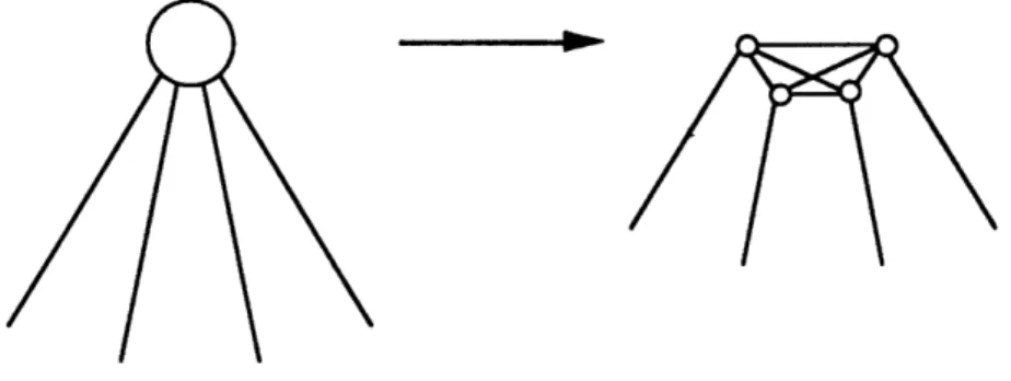
S of vertices. The proof of Theorem 2.1 is based on Lemma 2.2 - a stronger version of a result due to Lovasz [75] on connectivity properties of Eulerian multigraphs. The key concept in Lovisz's result is a splitting operation which, given two edges (x, u) and (, v), replaces (x, u) and (, v) by a new edge (u, v). The operation also plays a basic role in connectivity results of Rotschild and Whinston [96], Mader [78], Lovasz [75,76] and Frank

[36].

Lemma 2.2 Let G = (V,E) be an Eulerian multigraph. Let c(i,j) (i,j E V) denote the maximum number of edge-disjoint paths between i and j. Let x be any vertex of G and let u be any neighbor of x. Then there exists another neighbor of x, say v, such that,

by splitting off (x, u) and (x, v), we obtain a multigraph G' satisfying the following two conditions:

2. CG(x,j) = min(ca(x, j),dG(x)-2) for all j E V \ {x}, where dG(x) represents the

degree of vertex in G.

Condition 2 states that the splitting operation can be performed while maintaining most connectivity requirements involving vertex z.

Proof of Lemma 2.2:

Lovasz [75] proves a slightly weaker version of Lemma 2.2 in which condition 2 is not present. His elegant proof proceeds along the following lines.

1. There exists at most one set S satisfying: (a) ES, u S,

(b)

16(S)l

x,

2. If there is no such S, then any neighbor v of x can be used for the splitting operation. 3. If such an S exists then there exists at least one neighbor of x in S. Moreover, any

neighbor of x in S can be used for the splitting operation. Our proof of Lemma 2.2 directly rests upon Lovisz's proof.

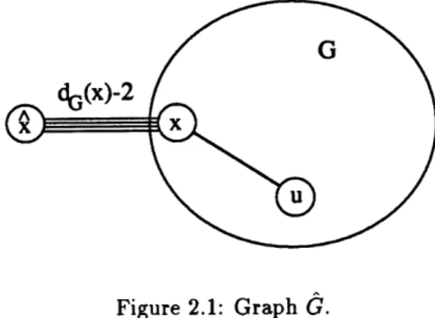
If dG(x) = 2 then the result follows directly from Lovcisz's result. Hence, assume that dG(x) > 4. Let ( = (, E) be obtained from G by adding a new vertex i and by linking that vertex to x through dG(x)- 2 edges (see Figure 2.1). Clearly, 6 is Eulerian. Moreover,

cd(i, j) = CG(i, j) i,j E V

\

c,(i,j) = min(CG(x,j), dG(x)- 2) j E V

\

Using the first step of Lovisz's proof, we obtain that there exists at most one set S C

V U {)} satisfying

(a) x ES, u S,

Figure 2.1: Graph G.

(c) S is minimal with respect to the above two conditions.

If such a set S exists we see that E S. Indeed, if i

0

16(S)I

> dG(z) since

both u and i 0 S, and G is Eulerian. Moreover, 16(S)l would be equal to c6(i, i) for some

i

S \ {x}. This follows by (b) and the fact that

U {i))l <

16(S)I

which implies that

16(S)l

<

Moreover, if a set S satisfying (a)-(c) exists then there must exist some v E S with v i such that v is a neighbor of x. Indeed, if S does not contain any neighbor of x other than i then 16(S)1 > dG(x) which certainly dominates c(i&,j). Hence, there would exist some i E S, x i i and j 0 S such that 6(S) = c6(i, j). This leads to a contradiction

since S \ {x, i} would separate i from j and

16(S

\

i)) <

16(S)I.

As a consequence, irrespective of whether a set S satisfying (a)-(c) exists, using parts 2 and 3 of Lov6isz's proof, we see that there exists some v i such that by splitting off

(x, u) and (, v) we obtain a graph G with c6(i,j) = co(i,j) for all i,j E V U {i} \ {x}.

By removing i, we get a graph G' which could have been obtained from G by splitting off

(x, u) and (x, v). G' satisfies

CG,(i,j) = c6(i,j) = c6(i,j) = cG(i,j) for all i,j E V \ {x}

cG'(X,j) = c6(x,j) > c(,j) = c&(ij)

Moreover, due to the splitting operation, cG(x,j) < cG(z,j) and cGa(z,j) < dG(x) - 2.

This completes the proof of Lemma 2.2. 0

We are now ready to prove Theorem 2.1. Proof of Theorem 2.1:

Clearly Z0

(r)

that ZO(r) > ZD(r) we consider an optimal solution, say , to (P.(r)). We shall construct a feasible solution y to (PD(r)) whose cost is at most equal to the cost of x. Since all data is rational, we may assume that all components of x are rational. Hence, there exists some integer k such that kxe and krij are even integers for all e = (i,j) E E. Let G = (V, E) be the Eulerian multigraph which has kz copies of edge e. By the max-flow-min-cut theorem, c(i,j) > krij for all (i,j) E E. As a result, by applying Lemma 2.2 repeatedly with z chosen among the vertices in D, we will eventually obtain a multigraph G' such

that

(i) cG(i, j)

> krij

(ii) dG'(i) = max krij i ED.

jEv\(i)

Therefore, if we let Ye (e E E) be equal to the number of copies of edge e in G' divided by k, we obtain a feasible solution to (PD(r)). Moreover, since the costs satisfy the triangle

inequality, each time we perform a splitting operation the cost of the solution does not increase which implies that

E

eEE eEE

proof of Theorem 2.1. 0

In general, when the costs do not satisfy the triangle inequality, the parsimonious prop-erty does not hold. Nevertheless, this is not a restriction for the survivable network design problem and its special cases, such as the Steiner tree problem or the k-edge-connected network problem. Indeed, let us consider an instance of the SNDP with arbitrary costs

{ce}. Define c (e = (i,j)) to be the length of the shortest path between i and j with respect to the lengths {ce}. Clearly, {ce} satsify the triangle inequality. Theorem 2.3 states that we can replace c by ce without affecting IZo(r) or ZO(r).

Theorem 2.3 For any set {ce} of costs, IZO(r) = IZO(r) and ZO(r) = Z(r), where IZ'(.) and Z'(.) refer to the costs {c').

Proof:

Since c' < c, for all e E E, IZ0(r)

IZO(r) and Zo(r) < Z(r). Now, consider an

optimal solution z* to (IPo(r)) (resp. to (Po(r))) with respect to the costs {c}. In order to construct an optimal solution with respect to the costs {ce}, we perform the following transformation. If some edge e = (i,j) with c < ce has some nonzero weight *, then we decrease z* to 0 and increase by x* the weights on the edges of a shortest path from i to

j. Notice that this maintains feasibility and optimality of the solution. By repeating this

operation, we obtain an optimal solution i to (IPO(r)) (resp. to (Po(r))) with respect to the costs {c'} such that i = 0 whenever c < c. As a result, the cost of this solution remains unchanged if we replace c' by ce. This and the fact that IZ0(r) < IZO(r) (resp. ZO(r) < ZO(r)) imply that i is also optimal with respect to {cc}. This completes the proof

of Theorem 2.3. 0

The above tranformation gives a generic transformation to convert a survivable network of total cost C' with respect to {c') into a survivable network of the same cost but with respect to {ce).

In order to illustrate a simple use of the parsimonious property, we now consider Gomory and Hu's synthesis problem [47]. Their problem is: given a symmetric matrix

r = [rij] of connectivity requirements, find capacities xij for all possible pairs such that,

in the resulting network, rij units of flow can be sent from i to j and the total capacity is minimum. In our setting, their problem is exactly the LP relaxation (PO(r)) with c, = 1 for all edges. Letting ri = max rij and C = ri, Gomory and Hu [47] show that C is a

lower bound on the total capacity of any feasible solution and present an algorithm which constructs a solution whose total capacity is exactly C, i.e. their algorithm produces an optimal solution. The fact that C is the optimal value can be seen very easily from the parsimonious property. Indeed ZO(r) = Zv(r) and these quantities are equal to:

Zv(r) = Min E z

eEE

subject to:

(Pv(r)) e > max rij S C V and S 0

: xe

=

eE6({i)

0

<

Summing up constraints (2.2) over all i, we obtain that any feasible solution to (Pv(r)) must have

Xe = Zri =C,

eEE s

implying that ZO(r) = C.

2.2

Extensions

The parsimonious property also holds if we have additional degree constraints in the problem formulation. Suppose that, in addition to the connectivity requirements, we impose that the degree of vertex i be at least ai for all vertices i in a subset T of V. To avoid trivial cases, we assume that ai > maxj rij. The integer programming formulation of this problem is:

IZT(r) = Min eXe

eEE subject to: s X,

>

0

> ai

Let (PT(r)) denote the LP relaxation of the above program and let ZT"(r) be its optimal value. In this context, we say that x is parsimonious at vertex i if

E

eE6({i})

ri = ai if i E T and ri = maxj rij if i T. By imposing parsimonious constraints at a

subset D of vertices, we define similarly (IPDT(r)), IZDT(r), (PDT(r)) and ZDT(r).

An interesting special case of this broader class of problems is obtained by letting

to (IP?)1 _{(2)) are almost k-tours. In fact, if we have the additional constraints xze 1 for} e E 6({1}), then these feasible solutions are precisely k-tours as defined in Section 1.3. As a result, IZ1}(2) is a lower bound on the value of the optimal k-tour, while Z1}(2) is a lower bound on the value Zkp introduced in Section 1.3.

Using the same argument as in Theorem 2.1, we can prove the analogue of the parsi-monious property in this more general setting.

Theorem 2.4 (The Parsimonious Property) If the costs {ce) satisfy the triangle in-equality then Z0 (r) = ZD(r) for all subsets D C V.

Theorem 2.4 will be used in Section 4.4 to strengthen Frieze's worst-case analysis [42] of a heuristic for the k-person TSP.

In general, it is interesting to investigate when a similar property holds for linear programs of the form:

Zo

= Min

E

ce

f(S)

where f is some set function. Generalizing Definition parsimonious at vertex i if

E

2.1, we say that a solution is

E Cede eEE E e > f(S) eE6(S) E Xe =f({i}) eE6({i)) O < X, SC V and S 0 iED eE E.