An albedo map and frost model of Pluto

AN ALBEDO MAP AND

FROST MODEL OF PLUTO

by

Eliot Fisher Young A.B., Amherst College (1984)

S.M., Massachusetts Institute of Technology (1987) S.M., Massachusetts Institute of Technology, (1990)

SUBMlTIED IN PARIIAL FULFILLMENT OF THE REQUIREMENTS FOR THE DEGREE OF

DOCTOR OF PHILOSOPHY

IN EARTH, ATMOSPHERIC AND PLANETARY SCIENCES

at the

MASSACHUSETI'S INSTITUTE OF TECHNOLOGY

September 1992

© Massachusetts Institute of Technology 1992, All Rights Reserved

Signature of the Author,

Certified by

-4

Accepted by

uepartment of Ear ospheric ahd Planetary Sciences September 16, 1992

Professor Richard P. Binzel Thesis Supervisor tmospheric and Planetary Sciences

Professor Thomas Jordan Chairman, Department Graduate Committee

ITHORAWN

_SpAgiFE

Acknowledgments

This thesis has been a collaborative effort. My committee members brought their various backgrounds to bear on the problems of mapping Pluto and modeling volatile transport from its surface, and I asked them a lot of questions.

I want to thank Jim Elliot for a careful reading of my thesis, Tim Dowling for

suggesting a spherical harmonic map in the first place, and Alan Stern for an intensive tutorial on icy satellites. I am particularly grateful to Rick Binzel for sharing his mutual event data set in the first place. I cannot list all of the things I've learned from my committee, but they will recognize the discussions we've had in these pages.

Other unwitting collaborators:

" John Spencer explained his Triton model to me. e Marc Buie discussed his mapping procedure. " Andy Ingersoll explained Io's supersonic winds.

" Dale Cruikshank explained the spectral features showing N2 and CO on Pluto. * After several discussions, Tony Dobrovolskis finally convinced me that the mutual event season happening at perihelion is a coincidence.

I owe the largest debt to my sister, Leslie Young. Nearly every idea in here has

benefited from her input. I also learned linear and nonlinear least squares fitting from her, the bread and butter of this thesis. Her atmospheric modeling [Elliot and L. Young,

1992] based on the 1988 stellar occultation by Pluto is crucial to the volatile transport

model of Chapters IV and V.

I am glad that my fianc6e is a former editor. Thank you, Diane.

Table of Contents

A bstract ... - -- - - . ---... page 4

Chapter One: Introduction ... _{page 5} Chapter Two: The Pluto Mapping Problem ... page 12

Chapter Three: Recent Least Squares Solutions...page ₂₅ Chapter Four: Volatile Transport Models ... page 50

Chapter Five: Short Term Frost Model Predictions...page 63 Chapter Six Summary and Discussion .--....---... _{page 98}

Appendix A: The Data Set...page ₁₀₀ Appendix B: Sm oothing the Maps...page ₁₀₂ Appendix C: Calculating Column Abundances...page ₁₀₃ Appendix D: Modeling the Reflectance of Thin Frost Layers...page 107 Appendix E: The Relation between Hapke and Minnaert Parameters ... page 114 R eferences...---.. _{---... ... page 122}

AN ALBEDO MAP AND FROsr MODEL OF PLUTO by

Eliot Fisher Young

Submitted in partial fulfillment of the requirements for the Degree of Doctor of Philosophy in Earth, Atmospheric and Planetary Science at the Massachusetts Institute of Technology, May 1992.

Thesis Supervisor: Dr. Richard P. Binzel, Associate Professor of Planetary Science.

Abstract

The once-per-century set of occultations of Pluto by its satellite Charon enable the construction of an albedo map of Pluto's sub-Charon hemisphere, which in turn provides a basis for models of volatile transport on Pluto. Photometric observations of the Pluto-Charon mutual events were obtained at the University of Texas McDonald

Observatory from 1985 through 1990. We use three least squares models to find the surface albedo distributions that best match the observed lightcurves. All of the least squares fits use a singular value decomposition (SVD) implementation. The three models produce similar albedo maps.

Features of the maps include a large, very bright region over the south pole, a dark band over the mid-southern latitudes, a bright band over the mid-northern latitudes. The average normal reflectance of the higher northern latitudes is about the same as Pluto's global average of 0.5. We do not find compelling evidence of a bright cap over the north polar region.

We model Pluto's atmosphere and albedo for the period from 1990 to 2040. Pluto's surface temperature drops by about six degrees during this period, resulting in over 97% of its current atmosphere condensing onto the surface. As Pluto's atmosphere thins, the winds arising from sublimation-driven pressure gradients increase beyond Mach 1. Our model predicts that the crossover to supersonic winds occurs around 2070. Our current frost migration model is valid only for the subsonic regime, but a supersonic frost transport model may help to explain the polar asymmetry of Pluto's albedo distribution. In the short term, the bulk of the new frost is deposited on the south pole. The change in albedo distribution is sensitive to the manner in which new frost reflectances are modeled, but the sheer volume of material (over 40 g/cm2) deposited mandates the

I. Introduction

Pluto is the only major planet that has yet to be visited by spacecraft. Our knowledge of other planets is sufficient to place them in the provinces of geophysicists and

atmospheric dynamicists, whereas Pluto's radius and mass were only recently

determined to better than a factor of two. This situation should change soon. A recently completed set of transits and occultations between Pluto and its satellite Charon

promises to make the next few years a golden age for the study of Pluto. This thesis uses lightcurves from these occultations to build a surface reflectance map of Pluto and makes 50 year projections for Pluto's surface temperature, pressure, albedo and column abundance.

A. The Pluto-Charon System

When Charon was discovered in 1978 [Christy and Harrington, 19781, its orbital plane around Pluto was nearly parallel to the line of sight from the Earth. Pluto's rotation rate had been known since 1954 from the periodicity of rotation lightcurves [Walker and Hardie, 1954]. While looking at astrometry plates, James Christy noticed an irregularity on Pluto [Figure 11 that moved with a period of 6.38 days, the same as Pluto's rotation period. The "bump" might have been a bright spot on Pluto's surface or a

satellite. In early 1985 the first transits were observed [Binzel et al., 1985], as Charon grazed across Pluto's north polar region. During the next six years a transit of Pluto by

Charon and an occultation of Charon by Pluto (collectively referred to as "mutual events") occurred nearly every Pluto day, equivalent to 6.38 Earth days. As shown in Figure 2, the path of Charon's transits migrated from Pluto's northern hemisphere to its southern one over this six year period .(We define "north" as the direction of Pluto's spin angular momentum vector.) We obtained mutual events lightcurves spanning this entire period. These provide coverage of the entire Charon-facing hemisphere of Pluto. Since Pluto's and Charon's orbits are mutually synchronous, Charon's transits always cover the same hemisphere of Pluto, which we refer to as "Pluto's sub-Charon

hemisphere."

5-Equatorial North, J2000 Coordinates

Figure 1. Photographic plate of Pluto and Charon circa 1978. This is one of the plates which led to the discovery of Charon by James Christy of the United States Naval Observatory (USNO). On the right side is a schematic of the system's orientation. Adapted from "The New Solar System," [Beatty and Chaikin, 1990].

1989-1990 1987-1988 1985-1986

Figure 2. Charon's path across Pluto migrates from period of the mutual events.

north to south over the six year

The angular separation between Pluto and Charon is only 0.9 arcseconds when Charon is at elongation. The pair can be resolved by a few exceptional groundbased systems or by the Hubble Space Telescope (HST). The currently accepted value for the

Pluto-Charon separation is 19640 ± 320 km, from speckle interferometry [Beletic et al,

1989]. Tholen and Buie [1989] have used the timing of the mutual events to complete a

nonlinear least squares fit for Charon's orbital elements and Pluto's and Charon's diameters, using Beletic's semimajor axis to scale the linear dimensions.

Table 1. Orbital and physical parameters for Charon and Pluto [Tholen and Buie, 1989].

Semimajor axis 19,640 ± 320 km

Eccentricity 0.00009 ± 0.00038

Inclination 98.3 + 1.3 deg

Ascending nodea 222.37 + 0.07 deg

Argument of periapsesa 290 180 deg

Mean Anomalyb 259.90 ± 0.15 deg

Epoch JD 2,446,600.5 = 1986, June 19

Period 6.387230 ± 0.000021 days

Pluto radius 1142 + 9 km

Charon radius 596 17 km

a Referred to the mean equator and equinox of 1950.0. b Measured from the ascending node.

Tholen and Buie have upgraded some of Charon's orbital elements in this table since the work on our maps was completed. In particular, the inclination was increased to

98.80, and Pluto's and Charon's radii were changed to 1150 ± 7 and 593 ± 10 km

respectively. Bear in mind that the quoted error for Pluto's radius, "1150 ± 7 km," is only the internal error generated from the least squares fit. The mutual event determination of both Pluto's and Charon's radii are scaled by Charon's semimajor axis, which to this date remains the most uncertain of Charon's orbital parameters. These changes in the inclination and the radii are minor compared to the discrepancy between the planetary radii of Tholen and Buie and the radii based on the 1988 stellar occultation [Elliot et al.

1989]. The stellar occultation estimates for Pluto's radius are generally 50 km larger than

the mutual event estimates. Part of the discrepancy arises from the question of whether the mutual events' first and last contacts refer to the solid surface of Pluto or to an optically thick layer of the atmosphere. Recent HST imaging of the Pluto-Charon separation, which seems to indicate a semimajor axis smaller than 19640 km, are also in conflict with the occultation results [Tholen and Buie, 1991]. Another possible source for the radii discrepancies is the way Pluto and Charon were modeled in the mutual events. The treatment of Tholen and Buie modeled Pluto and Charon as uniformly bright disks [Buie et al., 1992]. If Pluto and Charon are significantly limb-darkened, then the

-7-mutual event solutions would tend to underestimate their radii. We have run nonlinear

fits in which Pluto and Charon are modeled as limb-darkened disks, solving for Pluto's

and Charon's radii to semimajor axis ratios (R/a and Re/a) as well as a Minnaert limb parameter for both objects. This fit is based on four "superior" events (Pluto in front) and six inferior ones. Both superi6r and inferior events must be used in order to separate radii from the Minnaert limb coefficients. Pluto occults Charon with its entire physical radius, but may have a smaller apparent radius due to limb effects when it is transited

by Charon.

We normalize all ten lightcurves by their pre-event baseline points. We ignore the possibility that the sub-event and anti-event hemispheres of Pluto and Charon have different geometric albedos, and the fact that the pre- and post-event baselines should be fit by a slope, not a constant flux. Ideally the relative B-magnitudes of Pluto and Charon would be determined from their respective rotational lightcurves, and someday they will be. In the meantime we assume that Pluto and Charon's magnitudes are

constant duing both the superior and inferior events. The penalty for these assumptions is the high X2 per degree of freedom, which is nearly 20 (ideally it should be about one), and the large formal errors generated from the fit. Nevertheless, despite the large formal errors for R,/a and Rc/a, the major portion of the error in the estimates of the radii are due to the uncertainty in the semimajor axis.

Table 2. Nonlinear Fit for Pluto's and Charon's Radii and Minnaert Limb Parameters - a Preliminary Solution

Pluto radius/semimajor axis R,/a = 0.0606 ± 0.00022

Charon radius/semimajor axis R/a = 0.0327 ±0.00019

Pluto Minnaert parameter k, = 0.51 ± 0.02 Charon Minnaert parameter ke = 0.56 ± 0.02

Chi Square/degree of freedom 20 Table 3. Covariance Matrix

R, Rc k, kc

2.39674 x 10-9 1.09602 x 10-10 1.22581 x 10- 9.26265 x 10-8 1.09602 x 10-10 1.79196 x 10~9 -1.09742 x 10- 4.24156 x 10-9

1.22581 x 10- -1.09742 x 10-8 2.44027 x 10-5 2.25612 x 10-5 9.26265 x 10~" 4.24156 x 10-9 2.25612 x 10-5 2.25408 x 10-5

Table 4. Normalized Covariance Matrix R, R k, kc 1.0 0.05093 0.50309 0.39343 1.0 -0.05891 0.01494 1.0 0.96169 1.0

The internal errors from the least squares fit (i.e., the diagonal elements of the covariance matrix (Table 3)) are only 1/3 to 1/4 of the error due to the uncertainty in the semimajor axis measurement. When these uncertainties are propagated into the radii estimates, we get (recall that a = 19640 ± 320 km [Beletic et al., 1988]):

02(R,) = (19640 x 0.00022)2 + (0.0607 x 320)2= (4.32)2 km ₊ (19.42)2 km = (19.9)2 km

and

a2(Rc) = (19640 x 0.00019)2 + (0.0327 x 320)2 = (3.73)2 km + (10.46)2 km = (11.1)2 km.

So R, = 1190.7± 19.9 km and R, = 642.2 ± 11.1 km.

The value of 1190 ± 20 km is consistent with the extrapolated estimates for Pluto's radius based on the 1988 stellar occultation [e.g. 1206 ± 11 km, [Elliot and L.Young,

19921), and the value of 642 ± 11 km, while larger than any previous estimates, is

consistent with the lower limit of 601.5 km associated with the Charon occultation recorded by Walker [Elliot and L.Young, 19911. The limb parameters are not highly correlated with the radii to semimajor axis ratios, but are highly correlated with each other. The limb parameters are close to 0.5, indicating no limb effect for Pluto and only slight limb darkening for Charon. It is a little surprising that the Minnaert parameters turn out to be so close to the non-limb darkened (uniform disk) case, yet the radii from the fit are 40 km larger than those of Tholen and Buie given a semimajor axis of 19640 km. The difference between our radii and those of Tholen and Buie seem to be data, not model driven. Until we resolve the differences between the two data sets, we will stick with the parameters of Tholen and Buie as listed in Table 1.

As a sensitivity test of the radii we generated two normal reflectance maps, shown here in a side by side comparison.

-9-Rp = 1142 km, Rc = 596 km

Figure 3. Side by side comparison of spherical harmonic maps generated from the usual parameters (R, = 1142 km, R = 596 km) (Right) and the parameters

from the preliminary nonlinear least squares model incorporating Minnaert limb darkening (left).

Both maps in Figure 3 are the results of identical inversion processes. The maps primarily show differences in the longitudinal placement of features. The map on the left also shows a dark band on the western limb, indicating that the model Pluto was uncovered when the lightcurve was in the flat baseline phase. This would require the

exposed part of the western limb to be dark, since it must not be a contributor to the lightcurve.

The dark western limb makes the model based on the larger radii less plausible. Until we improve the nonlinear fit parameters, we will continue to use the mutual event parameters of Tholen and Buie 119881.

B. The Utility of the Mutual Event Lightcurves

During an occultation of Pluto by its satellite, the total brightness of the system will decrease, depending on the brightness of the regions of Pluto that are obscured by Charon and its shadow. Six mutual event lightcurves (inferior) are shown in Figure 4. These lightcurves are the data set on which the albedo maps derived here are based.

Mutual Event Lightcurves (1985 -1990) 1.05 .+ - 0.85 0~ 4+ o 0.7 -s

~

0.75o 17 Feb 85 A +* . 20 Mar 86 + 22 May 87 -0.65 --- tt ! 0.65 18 Apr 88 + 30 Apr 89 : 24 Feb 90 -0.55 -3 -- 10 1 2 3

Hours from mid event

24FEB1990 30APR1989 18APR198 22MAY1987 2 MAR196 17 FEB 1985

Figure 4. Six lightcurves of occultations of Pluto by Charon. These lightcurves were measured at approximately yearly intervals from 1985 through 1990. All six lightcurves are courtesy of Richard Binzel.

Figure 4 shows that a central event lasts a little over four hours from first to last contact, and the depth of the event could be as low as 60% of the baseline flux.

Charon's orbital elements enable us to project Charon's position over Pluto's surface for every observation in the six lightcurve set. The decrease in brightness for that

observation tells us how bright the covered region on Pluto must be. With enough observations we can piece together a mosaic of the entire sub-Charon hemisphere of Pluto. This mapping procedure is the topic of Chapters II and III.

We assume that Charon's contribution to the lightcurve is a constant for every observation. Separate lightcurve photometry of Pluto and Charon is barely possible from the HST. Resolved images of Pluto and Charon in the 2.2 micron band have yielded magnitudes for opposite hemispheres of Charon (a rather sparse lightcurve, but useful

-for the mutual event geometry), but a similar analysis in the B or V bands has not been completed as of this writing [Bosh et al., 1992]. Charon rotates only 120 during an event, so roughly 2% of Charon's disk disappears off the east limb as another 2% rises over the west.

Because a Pluto's albedo is likely to be closely related to recent condensation or sublimation of frost, an albedo map of Pluto provides an opportunity to determine large scale, seasonal climatology on Pluto. Volatile transport models have already been developed for other icy satellites, notably Triton [Spencer and Moore, 1992] and lo [Ingersoll et al, 1985]. We believe that Pluto, like Triton, has a global atmosphere, the temperature and surface pressure of which are governed by the transport of volatiles over the surface. Some of the bulk atmospheric parameters can be taken from the analysis of the 1988 stellar occultation [Elliot and L.Young, 1992]. This occultation yields surface temperature, pressure and column abundances given the identification of N2 as the primary volatile in Pluto's atmosphere [Owen et al., 1992] [Cruikshank, 1992]. The Triton model, Plutonian atmospheric predictions, and results of the volatile transport model are the subjects of Chapters IV and V.

II. The Pluto Mapping Problem

To make an albedo map of Pluto from mutual event lightcurves, one keeps track of how the Pluto-Charon system brightness changes as parts of Pluto are covered or uncovered. The change in brightness tells us the relative brightness of the covered parts. The challenge is to reconcile all of the covered parts, which generally have banana-like or semi-circular shapes, into a single reflectance map of Pluto's surface. This chapter outlines issues in the lightcurve inversion problem for the Pluto-Charon system by taking a chronological survey of work in this area. We begin with two maps that were constructed without mutual event data.

A. Rotation Lightcurves:

The Two-Spot Model [Marcialis, 1988] and The SHELF Model [Buie and Tholen, 1988]

Rotation-based maps are poorly constrained in latitude. If the axis of rotation is not perpendicular to the observer's line of sight, then much of the rotating body may never come into view, and the lightcurve may show almost no variation with rotation. Even if the axis of rotation is perpendicular to the line of sight (as is currently the case with

Pluto), the rotation lightcurves do not produce a unique surface map, as Wild [1989] points out. For example, the following two albedo distributions both could be solutions to the same rotation lightcurve.

S S

Figure 5. These two different albedo maps produce identical rotational lightcurves if viewed from a sub-equatorial point of view.

One can obtain better resolution in latitude if rotation lightcurves from different viewpoints are available. In Pluto's case, the lightcurve of Walker and Hardie [1954]

provides a significantly different orientation [Figure 6].

13-Southt.

SSouth

Pole

Earth's North Pole of J2000

1985

1954

Figure 6. Pluto's orientation as viewed from the Earth in 1954 offers a more polar view than the current orientation.

If one were making a map from a 1985 and a 1954 lightcurve, one could get

latitudinally resolved information about each pixel from the different pixel projections in the two cases. The "arctic circles" would still only be resolved in longitude, but the area of these regions could be reduced by including more recent (e.g., 1964) lightcurves in the data set. A latitudinally resolved albedo map can be determined from noise-free rotation lightcurves [Drish and Wild, 1991]. The problems arise when trying to invert noisy lightcurves. Because pixel albedos are determined from small differences in their projected contributions to Pluto's overall albedo, adjacent pixels are highly correlated, and noise between consecutive points in a lightcurve wreaks havoc on the pixel solutions. In theory one can generate maps with good resolution in latitude, but in practice these maps will have banana-shaped features running parallel to lines of longitude and non-unique solutions due to the high degree of correlation between adjacent pixels. To lessen the correlation between pixels, one needs lightcurves in which pixels are alternately completely visible (not just projected slivers) and then completely covered. The transits by Charon are the best source of this type of lightcurve.

The use of 20 and 30 year old lightcurves implicitly assumes that Pluto's albedo distribution has remained constant over that period. In Chapters IV and V we calculate resurfacing rates for most of Pluto in excess of ± 1 g/cm2 per decade, easily enough to change Pluto's albedo. Buie et al. [19921 have noted that the contributions to his model's x2 _{from each rotation lightcurve data point is six times that of each mutual}

event lightcurve point.

In the Two-Spot Model the size, location, and albedo of two spots on Pluto's surface are free parameters in a least squares fit. The advantage of a spot model is that it

from the available data set. The disadvantage is that Pluto's surface, in reality, may not have large spot-shaped features. Nevertheless, in the face of limited data, the spot model approach is a viable way to solve an underdetermined problem. The Two-Spot Model uses four parameters to describe the spots: two spot radii, a single latitude for both spot centers, and a longitude offset between the two spots. These parameters are called R1,

R2, LAT, and DLON respectively. Another parameter, ALBFAC, defined as

1 - (spotted albedo / unspotted albedo), describes the albedo of the spots (a single parameter) relative to the background. Finally several polar cap models are tried, loosely constrained by the secular dimming and increase in rotational variation of Pluto's lightcurve since 1954. The polar caps and the two spots are determined independently from secular dimming effects and from rotational lightcurves. Marcialis' adopted model is shown in Table 5.

Table 5. Adopted parameters for the Two-Spot Model, adapted from Marcialis

[19881.

R1

46

deg

R2 28 deg

LAT -23 deg from rotational lightcurves

DLON -134 deg

ALBFAC 0.9

J

N. Pole Limit 59 deg from secular dimming

S. Pole Limit -69 deg

Marcialis points out that the polar boundaries are poorly constrained in his model fit. It is important to note the large size of the north pole relative to the south. The model from Table 5 sports a north pole with approximately 175% the area of the south pole. Interestingly enough, the SHELF Model [Buie and Tholen] supports this same asymmetry, in contrast to the mutual event maps that would follow. Perhaps there was an expectation that a large frost cap would have developed on the north pole because it was in perpetual shadow during the approach to perihelion.

The SHELF Model [Buie and Tholen, 1988] is also a four spot model (the Two-Spot Model has four spots counting the poles), but has a larger number of free parameters. Each spot is assigned an independent radius, central latitude and longitude, a single scattering albedo, and an average particle phase function (evaluated at a scattering angle of 180*). The single scattering albedos and phase functions of Charon and Pluto's background constitute four more parameters, for a total of 24. The south polar spot is locked directly over the south pole, reducing the number of free parameters by 2. Pluto's

15-overall intensity is computed using the Hapke bidirectional reflectance equation, which is Eq. (16) from Hapke, 1981.

r(go, g, g) = g {[1 + B(g)]P(g) + H(go) H(p) -1) (1)

4c o + Ji

where r = ratio of bidirectionally reflected to incident flux,

w = single scattering albedo

g = phase angle (angle between the incident ray and the ray to the observer)

= cos(emitted ray) g= cos(incident ray) P = phase function

H = approximation to Chandrasekhar's H-function, of the form

H(g )=

a

1

I+R(2)

+

2ft

(2)

and B(g) = the backscattering function,

B(g) = B 1 -t (3 - e-h/tanlgl)(1 - e-h/tangl) (3)

where the B0 parameter describes the opposition effect.

Bo

~ e-w2

/2 (4)

and h is a packing parameter.

This expression for the intensity is a nonlinear function of w and P(O). Buie and Tholen use a simplex algorithm to search for the minimum X2 [Press et al, 19881. In my

experience the simplex algorithm is suitable for systems with a small number (e.g., three or four) of parameters but not for larger systems, since it is very slow and often stops prematurely. Nevertheless, Buie and Tholen, starting from three different arrangements of spots on the planet's surface (called MIN, MAX, and SHELF) find two local x2 minima. Two of the initial spot distributions, MIN and SHELF, converged to the same solution. Although no mutual event lightcurves were included in the data set, they were used to choose qualitatively between the simplex method's two local minima. The SHELF model was judged a better fit to mutual event data than the MAX model.

Table 6. Spot Model

[19881.

Parameters for SHELF, adapted from Buie and Tholen

Radius (kim) w P(0)

Plutoa 1162.0 0.776 2.1

Charonb 620.7 0.863 1.

Spot Latitude Longitude Radius w P(0)

#1 -1.9 110.1 30.6 0.406 0.4

#2 -23.0 195.2 14.8 0.971 2.9

#3 81.4 195.6 59.4 0.999 2.2

#4 South Pole 44.2 1.000 1.5

a These are the unspotted properties of Pluto.

b These are the global properties of Charon.

The radii of 1162 km and 620 km are based on a semimajor axis for Charon of 19800 km. (The following paper in the same issue of Icarus is by Beletic et al. [1988], in which the authors (Tholen and Buie) revise the speckle value for Charon's semimajor axis to be

19640 ±320 km.) The SHELF Model is shown in Figure 7.

Bright and dark equatorial spots of the SHELF model

Figure 7. The SHELF model, Jan 23, 1988 (with Charon emerging from eclipse), adapted from Figure 9 from Buie and Tholen [1988]. Up in this figure is Equatorial north of J2000.

17-Summarizing the results of the Two-Spot Model and the SHELF Model, we find: * The polar regions are very bright. Both models fit Pluto with polar caps that have

geometric albedos of one.

e Both models find that the north polar is much larger than the south polar cap. In the next section we will see that this finding is at odds with the results of the mutual event maps.

B. Mutual Event Models:

The Eleven Panel Map [Young 1990], The ESO Map[Burwitz et al, 19911, and

The Maximum Entropy Map [Buie et al, 19921

The three maps discussed in this section use mutual event lightcurves to provide resolution In latitude for the sub-Charon hemisphere of Pluto. One of them, the

Maximum Entropy Map, also uses mutual events ('superior' events, meaning that Pluto occulted Charon) to get better resolution of Charon's sub-Pluto hemisphere. The other maps are only concerned with Charon during the six hour duration of an event, so they assume a constant magnitude for Pluto's satellite.

The Eleven Panel Map was the first to detect Pluto's surprisingly bright south pole. Previous maps indicated that Pluto's south pole is smaller and darker than the north polar region.

The Eleven Panel Map divides the sub-Charon hemisphere of Pluto into four bands of latitude. Each of these is divided two or more times in longitude. The normal

reflectance of each panel is a free parameter, for a grand total of eleven free parameters. Once the relative brightness of each panel is found, all of the parameters are scaled such that the total area-averaged normal reflectance is equal to 0.49. Pluto's observed sub-Charon geometric albedo Is 0.49 [Mulholland and Binzel, 1984], and the normal reflectance is equal to the geometric albedo given a Minnaert limb parameter of 0.5. We used a linear least squares fitting algorithm to solve for a surface albedo distribution. This gives the model an advantage in speed and convenience, but necessitates leaving

out nonlinear physical processes, such as Hapke surface scattering. Minnaert limb-darkening can be incorporated in a linear model and has been included in the Eleven Panel Map.

(D0

N

0

Figure 8. The least squares solution to the eleven panel map. Gray scales illustrate the normal reflectances for each panel: white = 1, black = 0.

Table 7. The Eleven Panel Map [Young, 1990] [Young and Binzel, 1990]

Panel Normal Panel Normal

Reflectances Reflectances A ... 0.69 ±0.041 G...0.33 ±0.030 B...0.43 ±0.045 H ... 0.25 ±0.023 C...0.57 ±0.023 I...0.37 ±0.027 D...0.50 ±0.022 J...0.87 ±0.034 E ... 0.58 ±0.022 K ... 0.81 ±0.043 F...0.53 ±0.028

It is worth mentioning why our maps are in terms of normal reflectances, as opposed to geometric albedos or bidirectional reflectances. Geometric albedo is a quantity defined for an entire sphere; namely, the ratio of light reflected by a planet relative to that reflected by an isotropic, perfectly reflecting disk of the same apparent size. We could talk about "local geometric albedos," but that would stretch the definition of geometric albedo. Bidirectional reflectance is locally defined [see Equation 1], but has values that are nonintuitive. For example, regions of Pluto that have normal reflectances of 0.8 - 0.9

may have bidirectional reflectances in the neighborhood of 0.15. The lower values are due to the definition of bidirectional reflectance. We use the normal reflectance instead.

19-The overall normal reflectance is easily related to the geometric albedo [Veverka et al.,

1986, p. 377]:

r. = (0.5 + k) p (5)

where rn is the normal reflectance,

k is the Minnaert limb-darkening parameter [see Equation 7], and p is the planet's geometric albedo.

The quoted errors in Table 7 are the formal errors of the least squares problem. Specifically, the error in the it parameter is

i= m CovIi, i] (6)

where n is the number of observations, m is the number of parameters,

x2 _{is the sum of the squared weighted residuals, and}

Cov[i, 1] is the it diagonal element of the covariance matrix.

The Minnaert limb parameter, k, relates the intensity from the limb of a planet to the intensity at the center of the disk.

I = Iocos2k-i()

(7)

where I is the intensity of the center of the planet's disk,

k is the Minnaert parameter, and

o

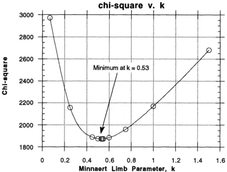
is the angle between the surface normal at the disk's center and the normal anywhere else on the planet.

We estimate the limb parameter by trying a range of values from k = 0 to k = 1.5 and

plotting

x

2

chi-square v. k

3000-e 2600 - - - ---Minimum at k 0.53 C* 2400 - - --- --- - .- .- --- - - -2200 - --- --- - -- - -- -2000 -

---1800

0 0.2 0.4 0.6 0.8 1 1.2 1.4 1.6

Minnaert Limb Parameter, k

Figure 9. X2 as a function of k, the Minnaert limb parameter. A value of k = 0.5

indicates no limb-darkening effect. The minimum at k = 0.53 indicates

only a slight amount of limb-darkening.

It should be no surprise that the best fit limb parameter is close to 0.5, since Tholen and Buie [1989] assumed non limb-darkened disks in their model. On the other hand, our preliminary nonlinear fit (which allowed for possible limb-darkening) found a limb coefficient of only 0.51 ± 0.022 for Pluto [Table 2]. In general one expects bright objects like Pluto or Europa to be strongly limb-darkened (for Europa k is about 0.70 [Veverka et al., 19861), while the moon is not limb-darkened (k = 0.5). If Pluto does possess a haze

layer, one might expect Pluto to be limb-brightened, because the projected optical thickness of the haze is greatest at the limbs, and the haze might be more effective at reflecting light at the limb. The optical properties of the lower atmosphere are unknown at this time, so the limb coefficient cannot be interpreted as if it is solely due to Pluto's surface.

The optical thickness of a possible haze layer brings up the question of whether the variation in the mutual event lightcurves is due surface features of atmospheric

phenomena. The column abundances of methane, N2 and CO are so low that we certainly see through them to the surface, unless there are aerosols suspended in the lower atmosphere [Cruikshank et al., 19891. A limb coefficient of less than 0.5 (indicating

-limb brightening) would have been evidence for an optically significant haze layer. The best evidence that we actually see surface features as opposed to, say, clouds is the

long-term repetition in Pluto's rotational lightcurves.

The brightest region of the Eleven Panel Map is the south pole, panels J and K. The darkest region is the adjacent band, panels G, H, and I. The north pole, panels A and B, have an average brightness that is about the same as Pluto's global albedo of 0.5. The Eleven Panel Map's north and south pole albedos contradict the resultsfrom the

Two-Spot Model and the SHELF Model .The other mutual event maps also contradict the rotation-based maps.

The European Southern Observatory Map is written up in the December 1991 issue of the ESO Messenger [Burwitz et al, 1991]. The ESO Map is a finite element map, like the Eleven Panel Map, except that it has 17 surface elements and has been smoothed. The authors remark on the surprising polar albedos of their map:

Our albedo map reveals that areas of high contrast must coexist on the Charon-facing hemisphere of Pluto. The highest contrast found was that between the two polar caps. While the south polar region appears to be the brightest area on the planet, we found that the north polar region has the lowest albedo [Burwitz et al, 19911.

The latest map by Buie et al. [19921 uses a maximum entropy method to solve for pixel albedos on Pluto's surface. The maximum entropy method (MEM) is similar to a least squares technique in that both seek to minimize a merit function of some kind, usually the weighted sum of squared residuals. The difference is that the MEM tries to maximize a quantity called the entropy under the constraint that X2 is less than or equal to a target value, Ca. Optimally Cair should be unity, but it is not always possible to reach arbitrarily low values of Cai.

One maximizes S subject to the constraint C < Ca. If the unconstrained maximum

of S satisfles this constraint, then this will be the maximum entropy solution -the data are too noisy for any information to be extracted. Otherwise the solution will lie on the boundary C = Cair and we have an optimization problem with an equality constraint to solve. [Skilling and Bryan, 19801.

The entropy, S, is defined as the negative of the information content of a probability distribution.

S = pi log (8)

where p, is the it parameter, normalized to the range from 0 to 1, and m1 is some kind of initial estimate.

data sets that do not completely constrain the solution. Of the infinite number of solutions that would fit the data equally well, the MEM finds the one for which the information entropy is a maximum. Why is this particular solution a good choice?

Consider the Kangaroo Problem:

Suppose we know two things about kangaroos: * One third of kangaroos have blue eyes. e One third of kangaroos are left handed.

Now, what is the most reasonable probability that a kangaroo will be both left-handed and have blue eyes? We build a 2 x 2 sample space of the problem.

left-handed left-handed left-handed

T F T F T F

True 1/9 2/9 1/3 0 0 1/3

.R False 2/9 4/9 0 2/3 1/3 1/3 uncorrelated positive negative correlation correlation

Figure 10. Sample space for the Kangaroo Problem.

There are many possible sample spaces that fit our knowledge of the kangaroo situation, but these three cases cover the extremes. In the absence of any information (e.g., are the genes for left-handedness and eye color on the same chromosome), the best choice for the sample space is the uncorrelated case. Now suppose we try to find the best set of probabilities not by inspection, but maximizing the entropy. Only when we

maximize the entropy do we get the uncorrelated result . The entropy in Figure 10 is

1.27, 0.63, and 1.01 for the uncorrelated, positively correlated, and negatively correlated

cases respectively. The entropy of the uncorrelated case is the highest. A solution in which some parameters are correlated represents an application of knowledge where none is justified by the data.

We can pose the albedo reconstruction problem as follows: divide Pluto's surface into a grid of surface elements, and let the albedo of each element be a free parameter. With any reasonably ambitious grid (e.g., 20 x 40), the solution will be underdetermined since there is not enough information to pin down the albedo of every pixel. We may know the sum of two adjacent pixels, but not know the distribution between them. There are an infinite number of solutions, but we want the one in which the pixel values are uncorrelated.

Buie et al. cast Eq. (8) in terms of the image value at each surface element.

-N I' S

= I Ij - Dj

- Ij-1 -j(9)

j = 1

where I, is the image value of the j* surface element,

DI Is the associated default value, and

N is the number of surface elements in the model.

The black art in the maximum entropy algorithm is in picking an expression for the default value, D,, since it defines the entropy and will shape the solution in regions of poor data constraints. Often D, is defined as the average image value based on the entire image [Skilling and Bryan, 1984]. Buie et al. use a more local definition of D,; they define it as the average of a pixel and its eight neighbors. I suspect that this helps the MEM find a solution with sharper features. Notice that the MEM solution given Cam and a definition of Dj is unique, but, since D, can be defined different ways, there is not a unique "MEM solution" to a problem.

The results of Buie et al. confirm the results of the Eleven Panel Map and the ESO Map. They also find a bright south polar region and do not find a bright north polar region. "...a south polar cap is evident in the map of Pluto. The north polar region is brighter than the equatorial regions but is not as bright as the south pole [Buie et al.

III. Recent Least Squares Solutions

This chapter describes three separate linear least squares models of Pluto's surface albedo [Young and Binzel, 1992]. Each model introduces some structure into the solution, so comparisons from a set of solutions help us recognize features that may be artifacts of one particular model. This is the motivation for using three distinct models, which are

" The Spherical Harmonic Model, " The Polynomial Model, and e The Finite Element Model.

In all three of the models the free parameters appear as linear terms. The advantage of linear models is speed; a least squares fitting routine will find a solution in a single iteration. A clear explanation of the linear least squares problem is given in section 14.3 of Numerical Recipes (either C or Fortran versions) [Press et al. 1988].

The three models all have a similar form, representing Pluto's apparent intensity as:

N

1(t)

=

YX

pi

xi(O,<;t))

(10)

i =1 all 9, $

where I(t) = Pluto's intensity at time t,

N = number of parameters in the model,

p, = the i* parameter, and

= the it basis function.

The basis functions are functions of latitude and longitude as well as functions of time, since they incorporate the temporal effects of Pluto's rotation and the coverage by Charon and its shadow. For example, consider a set of spherical harmonics. The basis function X(O,$;t) is identical to the i* spherical harmonic, YLM(,$), except that each point on Pluto is attenuated by a projection factor, and points that are hidden by Charon or its shadow or behind the limb of the planet at time t are simply zero. Charon's coverage and the projected area of a patch on Pluto's surface are clearly time dependent phenomena; thus X is a function of t, even though the i"' spherical harmonic is not. A comparison of Eq. (10) and Eq. (14) shows that the basis functions X(O,5;t) are really the product of some function that is defined on a sphere (like YLM(O,$)) and the exposed, projected area of the surface element at 0,$ at time t (otherwise known as g(O,$;t)). Each basis function is evaluated on a 100 x 100 grid covering Pluto's

-Charon hemisphere. Because Pluto rotates 12*- 150 during an event, we extend the grid slightly beyond the sub-Charon hemisphere, from 97.5*W to 97.5*E. Although Charon never transits longitudes beyond ±90*, those longitudes of Pluto are visible during an event. The extent in latitude is from 900S to 90*N.

The total model contribution is the linear combination of all the basis functions evaluated at all of the grid elements with each grid element's projected area scaling the function's value. The projected area of an infinitesimal grid element is

da

=

(n 'p)r

2

_{cose dO dp}

₍₁₁₎

where 0 = latitude, $ = longitude, r = planetary radius,

dO, do = pixel's extent in latitude and longitude,

n = the normal vector from the planet's surface at 0,4$, and

p = unit vector defining the projection plane. The normal vector's components are

n = cos0cos$,

ny = cos0sin$, nz = sinO.

It is important that the normal to the projection plane, 9, be in the same coordinate system as the surface normal vector ^n (generally Pluto's local coordinate system). The vector ^ points from Pluto to the Earth.

What is the process of finding the least squares solution? We start with a merit

function as the measure of the quality of the fit, defined to be the weighted sum of

squared residuals, x

2_.

X

2

_-

_[Li

2

₍₁₂₎

where n = number of data points,

y, = the observed intensity for the i* timestep, ai = the error in y1, the i* observation, and

I, = the model intensity for the i* timestep.

equations) and then finding the parameter values that solve the normal equations. This

last step amounts to solving the matrix equation

[a] a = D ₍₁₃₎

where [a] = the design matrix,

7 = _{vector of least squares solutions for the n parameter values (i.e., the answers), and}

D = vector of weighted observations.

We solve for the parameters by inverting the matrix [a] in Eq. (13). If two of the parameters are closely correlated, or if the data set provides no means of distinguishing the contribution of one parameter from another, then the matrix [a] will be nearly singular, resulting in nonsense or a non-unique solution when we try to invert it. We deal with this likely possibility by using singular value decomposition (SVD) to invert the matrix [a]. When a matrix is singular, an infinite number of vectors a will satisfy Eq.

(13), since the contribution from one row of [a] is zero, regardless of the vector 7. The SVD is robust in this situation, and returns the solution that distributes power most

evenly among the correlated parameters. An advantage of least squares techniques, including the SVD implementation, is that they produce a correlation matrix that can identify correlated parameters. This ability turns out to be critical in selecting free parameters for the three models.

A. The Spherical Harmonic Map

The spherical harmonic model represents Pluto as a linear combination of terms

from a truncated spherical harmonic series.

Xi(0,$;t) = g(0,$;t) YLM(0,$) = g(0,$;t) 2L + 1 (L -M)! P(

47t~~ (+M)P'(cosO) eiMO (14)

V 47 4I (L + M)! where 0 = colatitude, $ = longitude,

g(0, 0;t) = _{the exposed, projected area of a surface area element at 0, 5 at time t.}

YLm(0,$) = _{the spherical harmonic of order L, M,}

and Pm(cosO) is the associated Legendre polynomial.

These terms are complex when M > 0, so the real and imaginary parts are effectively different basis functions. Alternatively, one could use an imaginary parameter set, in which case the imaginary part of each complex parameter is a free parameter in its own right. We do not require that both the real and imaginary parts of a spherical harmonic term be included in the fit. The free parameters are the amplitudes of the various

spherical harmonic terms (the p,'s in Eq. (10)). Our goal is to find the set of p,'s that,

-when multiplied by their respective spherical harmonic terms, yield a model of Pluto that best duplicates the observed occultation lightcurves.

Spherical Harmonic Series through 6' Order, Real Part

0

1

2

3

4

5

6=L

O

0

0@

S

@M

ID

CA)

0;

Spherical Harmonic Series through 6' Order, Imaginary Part

Figure 12. Imaginary (odd) part of the spherical harmonic series through the sixth order.

The question of which parameters to include in the model proved a difficult one. In many models based on series expansions, there is a clear point at which one can truncate higher order terms. This is not the case in the spherical harmonic

decomposition. The normalized correlation matrix shows that there are

familes

of highly correlated parameters, where the members of each family look similar. For example, Figure 11 shows that the (2,0), (3,1) and (4,0) even terms are members of the same family; all three functions are basically spheres with symmetrical north-south polar caps. Although these three functions should be orthogonal, the data set's coverage of Pluto's sphere is restricted to one hemisphere, and that hemisphere is resolved into only six bands. This limited coverage results in an inability to distinguish similar terms from

each other. Our solution is to discard all but the lowest order member of each family. These families are shown in Table 8, which lists pairs of parameters with cross

correlation coefficients with magnitudes larger than 0.95.

In the next section we will use polynomials of latitude and longitude as a basis set instead of spherical harmonics. The polynomial set is not orthogonal on a sphere even with complete coverage. Our solution is to check the relative sizes (condition number) of

-the singular values from -the SVD. The finite element and spherical harmonic set may also contain linear dependencies due to the uneven coverage by Charon's transits, so the SVD is essential in all of the least squares fits.

Table 8. Correlated parameters in the spherical harmonic solution. High Order Term

Y(6,6) odd Y(6,6) odd Y(6,5) odd Y(6,4) odd Y(6,3) odd Y(6,3) odd Y(6,2) odd Y(5,5) odd Y(5,4) odd Y(5,4) odd Y(5,4) odd Y(5,3) odd Y(5,3) odd Y(5,3) odd Y(5,2) odd Y(5,1) odd Y(5,1) odd Y(4,4) odd Y(4,3) odd Y(4,3) odd Y(4,2) odd Y(3,2) odd Y(2,2) odd Y(6,6) even Y(6,6) even Y(6,6) even Y(6,5) even Y(6,5) even Y(6,4) even Y(6,2) even Y(6,1) even Y(6,1) even Y(5,5) even Y(5,5) even Y(5,4) even Y(5,4) even Y(5,2) even Y(5,2) even Y(5,1) even Y(5,O) even Y(4,4) even Y(4,3) even Y(4,1) even Y(2,1) even Y(1,1) even

Low Order Term Y(5,5) odd Y(4,4) odd Y(5,4) odd Y(5,3) odd Y(5,2) odd Y(4,1) odd Y(5,1) odd Y(4,4) odd Y(4,3) odd Y(3,2) odd Y(2,1) odd Y(5,1) odd Y(4,2) odd Y(3,1) odd Y(4,1) odd Y(4,2) odd Y(3,1) odd Y(3.3) odd Y(3,2) odd Y(2,1) odd Y(3,1) odd Y(2, 1) odd Y(1,1) odd Y(5,5) even Y(4,4) even Y(3,3) even Y(5,4) even Y(4.3) even Y(5,3) even Y(5,1) even Y(5.2) even Y(5,0) even Y(4,4) even Y(3,3) even Y(4,3) even Y(3,2) even Y(5,0) even Y(4,1) even Y(4,0) even Y(4,1) even Y(3,3) even Y(3.2) even Y(3,0) even Y(1,0) even Y(0,0) even Correlation Coefficient 0.99 0.96 0.98 0.97 0.99 0.98 0.97 0.99 0.99 0.97 0.97 -0.96 0.98 0.96 0.99 -0.97 -0.96 0.96 1.00 1.00 0.99 1.00 0.98 0.99 0.97 0.96 0.99 0.96 0.95 0.98 -0.96 0.98 1.00 0.99 0.99 0.97 -0.98 0.97 0.98 -0.98 1.00 0.98 0.97 0.99 1.00

Table 9 shows the least squares solution for the spherical harmonic case. None of the 16 parameters has a singular value near zero. (More importantly, none of the

parameters has a condition number close to the computer's resolution. The condition number is the ratio of a singular value to the largest singular value.)

Table 9. Parameter list for the spherical harmonic solution.

Parameter value error singular value

Y(0,0) (even) 3.858 ± 0.11 1. 16e+03

Y(1,0) (even) -0.07 ± 0.02 1.75e+02

Y(2,0) (even) 1.278 ± 0.15 1.06e+02

Y(2,2) (even) 0.266 ± 0.40 7.00e+01

Y(3,0) (even) 0.599 ± 0.08 5.51e+0 1

Y(3,2) (even) 0.983 ± 0.06 4.70e+01

Y(3,3) (even) 0.617 ± 0.32 3.38e+0 1

Y(4,2) (even) -0.72 ± 0.15 2.99e+01

Y(5,0) (even) 2.605 ± 0.14 2.11 e+0 1

Y(5,1) (even) -0.71 ± 0.26 1.48e+01

Y(6,0) (even) 0.470 ± 0.32 1.24e+01

Y(1,1) (odd) -0.04 ± 0.02 1.08e+01

Y(2,1) (odd) 0.038 ± 0.08 7.77e+00

Y(3,1) (odd) -0.58 ± 0.07 2.53e+00

Y(4, 1) (odd) 0.467 ± 0.18 3.04e+00

Y(6,1) (odd) 1.220 ± 0.24 4.78e+00

The

x

2 per degree of freedom is 1.82 for the spherical harmonic model.

We pause momentarily to explain how the errors are determined for each point on the surface. The error of each parameter is estimated from the formal error of the least squares fit.

ai

= COv[i, i] (15)

n-N

where ai = the error in the i* parameter, n = number of observations,

N = number of parameters,

X2 = chi square, the sum of weighted, squared residuals, and Cov[i, i] = the i* diagonal element of the covariance matrix.

The errors at any point on the surface are calculated by propagating the parameter errors. If the albedo, s(O, <), at any point is given by

-s(0,

$) = Pi X(0, $)i + P2 X(0, )2 + ...+PN X(0, )N,

then the albedo's variance at that point is

G

2

(0,

0)

=

(X(e,

$)1y

i2

(pi) +

(X(e,

$2)Y a

2

_(p

2

) +

...

₍₁₇₎

+

(X(o,

$)N a2(pN) + cross correlation terms

where p, = the i* parameter,

X(O,

4),

= the it basis function evaluated at lat. = 0, long. =

and each cross correlation term (there are (N - 1)2/2 altogether) is of the form

as as

cross corr. error = 2p - a(p) O(pj), (18)

api

a-Cpj

TP(8

where p = the (i,,j) element of the normalized covariance matrix.

The solution maps (Figures 15, 16 and 17) show that the errors near the limb are much larger than the errors for the rest of the planet. The solutions are problematic near the limb because of the geometry of the events. The east and west limbs are visible only for the first and last parts of an event; they rotate out of and into view as the event progresses. The extreme east and west longitudes (from 97.5* to 900 E and from 90* to

97.5* W) are never occulted by Charon, but must be included in the model because they

are visible during the early and late stages of an event. Furthermore the north and south limbs are only occulted roughly half the time, since the 1985-86 events hide the north pole and the 1989-90 events hide south pole. Since the limb regions are marginal

contributors to the overall lightcurve, the least squares solution can be absurdly high or low in those areas without affecting the total x2 _{very much. A partial solution to this}

problem is to include as many early (1985-86) events and late (1989-90) events as possible. In the meantime, we have to be skeptical of the albedo solutions found for the limb regions. It may also be the case that there is an optically thick layer that obscures more of the planet near the limb.

B. The Polynomial Map

The polynomial model has as its basis function polynomials of latitude and longitude.

Xi(0,$;t) = g(0,$;t) Pa,b(0$)= g(0,$;t) 0a b (19)

where 0 = latitude, * = longitude, a and b are integers, and

g(0, $;t) = the exposed, projected area of a surface area element at 0, $ at time t.

The free parameters are amplitudes of the polynomial functions (the p,'s in Eq. (10)). The set of polynomial functions are illustrated in Figure 13.

Polynomials of Latitude and Longitude through 8' Order

LatitudeOrder

2 3 4 5 6 4 5 6 7 8 Figure 13.

Although Figure 13 shows polynomials through 8t order, we only included terms up

-through sixth order in the actual polynomial model. Given only six transits by Charon, any higher order terms would over-fit the data. We observed singular values that were zero or very small when we included 7th and 8th order terms, indicating that the additional terms were not improving the model's ability to fit the data.

In contrast to the spherical harmonic model, the sixth order polynomial model only has 2 pairs of terms (out of 28) with cross correlations of 0.95 or higher, as opposed to the spherical harmonic case, which has over 30 pairs (out of 49 total). The amplitudes of even the most highly correlated terms are of reasonable size in the polynomial case, whereas in the spherical harmonic case there often are delicately balanced amplitudes

one hundred times larger than the rest of the set. The two correlated parameters are shown in Table 10, and the least squares solution for the polynomial model is shown in Table 11. As before, we keep only the lowest order parameter in each cluster of correlated

parameters.

Table 10. Correlated Parameters in the 6th Order Polynomial Solution.

High Order Term Low Order Term Correlation Coefficient LatA * LonA6 LatA0 * LonA4 -0.97

Table 11. Parameter list for the polynomial solution.

Parameter value error singular value

LatAO * LonAO: 0.920 0.04 5.03e+03

LatAO * LonA1: 0.207 0.09 9.96e+02

LatA * LonA0: 3.887 0.21 6.50e+02

LatAO* LonA2: 0.191 0.20 1.77e+02

LatA * LonA1: -0.431 0.27 1.50e+02

LatA2 * LonAO: -1.906 0.67 1.35e+02

LatAO* LonA3: 0.098 0.19 9.37e+01

LatA I* LonA2: -0.212 0.30 7.43e+01

LatA2 * LonAl: -0.677 0.61 5.09e+0 1

LatA3 * LonAO: -12.24 0.81 3.84e+0 1

LatAO* LonA4: -0.213 0.14 3.30e+01

LatAl * LonA3: -0.057 0.39 2.52e+01

LatA2 * LonA2: 0.949 0.55 1.41e+01

LatA3 * LonAl: 0.380 0.37 1.09e+0 1

LatA4 * LonAO: 3.902 1.52 8.55e+00

LatAO * LonA5: -0.059 0.10 7.08e+00

LatA * LonA4: -1.327 0.28 5.44e+00

LatA2 * LonA3: -0.317 0.43 4.9 1e+00

LatA3 * LonA2: 1.734 0.31 4.41e+00

LatA4 * LonA1: 0.494 0.39 3.38e+00

LatA5 * LonA0: 6.748 0.48 6.56e-0 1

LatA * LonA5: 0.290 0.21 1.11e+00

LatA2 * LonA4: 1.116 0.35 1.63e+00

LatA3 * LonA3: -0.126 0.49 2.03e+00

LatA4 * LonA2: -1.789 0.34 2.61e+00

LatA6 * LonAO: -1.408 0.73 2.49e+00

The

X'

per degree of freedom is 1.53 for the sixth order polynomial model.

C. The Finite Element Map

The Finite Element Model [Young 19901 [Young and Binzel, 1991] divides Pluto into contiguous panels of latitude and longitude. The brightness of each panel is a free parameter in the least squares fit.

Xi(0,$;t) = g(0,$;t) P(O,$) (20)

where 0 = latitude, * = longitude, and

P,(0,$) is the brightness of the Ct _{h panel, the panel that encloses the coordinates (0,0).}

We divide Pluto into a 6 x 6 grid, or 36 free parameters. The 36 panel finite element solution is shown in Figure 14 and Table 12.

-Mercator projection of the 36 Panel Finite Element Map

90ON

6

5

4

3

1

97.5

0

_W

_97.5*E

90

0

_S

Table 12. Parameter list for the 36 panel finite element solution.

Parameter value error singular value

1 2 3 4 5 6 7 8 9 10 11 12 13 14 15 16 17 18 19 20 21 22 23 24 25 26 27 28 29 30 31 32 33 34 35 36 7.187 0.573 2.134 4.558 -2.048 5.968 0.754 0.818 0.796 0.732 0.688 -0.579 2.163 1.456 1.485 1.459 1.539 0.679 0.733 0.024 -0.020 0.255 0.574 0.148 3.656 1.612 1.179 1.266 1.818 1.647 16.18 0.842 0.210 0.955 4.111 -18.31 2.90 1.67 1.38 1.34 1.91 2.79 0.38 0.15 0.13 0.19 0.16 0.51 0.29 0.13 0.12 0.08 0.10 0.21 0.23 0.13 0.08 0.11 0.18 0.44 0.33 0.15 0.12 0.13 0.27 0.80 3.51 1.34 0.96 1.09 1.56 3.33 8.09e+02 1.16e+02 1.08e+02 5.89e+0 1 4.78e+0 1 3.99e+0 1 3.38e+0 1 2.66e+0 1 2.30e+0 1 2.14e+01 2.02e+01 1.48e+01 1.28e+01 1.18e+0 1 1.03e+01 9.84e+00 9.39e+00 8.28e+00 6.20e+00 6.26e+00 4.68e+00 4.09e+00 3.38e+00 2.84e+00 2.60e+00 1.96e+00 1.90e+00 1.36e+00 1.29e+00 1.06e+00 3.05e-0 1 7.99e-0 1 6.13e-01 6.71e-01 4.78e-01 4.89e-0 1

The X2 per degree of freedom is 2.01 for the finite element model with 36 free

parameters.

All of the maps, particularly the finite element map, demonstrate the effects of noise

in the lightcurves: bright and dark regions adjacent to each other with large swings in albedo. The small elements near the polar regions are especially sensitive to noise. We

-smooth the maps by convolving them with an adaptive Gaussian-shaped filter, described in Appendix B. The width of the Gaussian depends on the formal error of the pixel being smoothed, so regions with higher errors are smoothed more heavily. For example, the finite element map contains two adjacent panels, #35 and #36, with out-of-bounds refiectances of 4.1 and -18.3 respectively. Neither of these panels affects the smoothed map very much, however, because their projected areas are extremely small and their associated errors are high.

The spherical harmonic, polynomial and finite element maps are shown in Figures

15, 16, and 17. Each figure shows both the original and smoothed versions of the map,

as well as a contour map of the formal errors associated with the original map.

Smoothed

Errors

0.05 -0.15 0-0.05 5 - 0.5 -0.05-0.15 0-0.05 '0.45-0.5 0- 0.05 0.05-0.15 Normal Reflectance Gray Scale

Figure 15. Normal reflectance maps of Pluto showing Pluto's sub-Charon hemisphere.

Original

SC) 0 E C

E

(LL

CDw

Smoothed

Errors

Original

0 1

Normal Reflectance Gray Scale

Figure 16. Normal reflectance maps of Pluto showing Pluto's north pole.

- 39 --U) ( Iz 0.05 -0.15 0-0.05 - 0.05-0.15 0-0.05 -0.45-0.5 0-0.05 -0.05 -0.15

Smoothed

Errors

-_U 0 SC E

E

. E

E .2

.,.,

Normal Reflectance Gray Scale

Figure 17. Normal reflectance maps of Pluto showing Pluto's south pole.

D. The Extreme Poles

All three maps exhibit apparent artifacts at the poles: a localized bright area at the

extreme north pole and a dark area at the extreme south pole. The uncertainties at the pole are high, as discussed in Section A of this chapter. Is there a direct way to

determine the actual albedos at the extreme latitudes? In 1985 and 1990 Charon grazed over Pluto's north and south polar regions respectively. We can run "spot checks" calculating the average albedo of the covered portion of Pluto for an individual observation. At individual timesteps, we compare the area covered to the fractional

decrease in brightness relative to the pre- or post-eclipse baseline value. The ratio of the fractional decrease in brightness over the fractional decrease in exposed area is equal to the albedo of the covered region relative to Pluto's average albedo. The fractional area

Original

0.05-0.15 0-0.05 -0.05-0.15 0 - 0.05 - 0.45-0.5 0-0.05 00-0.15