A Computational Model to Connect Gestalt Perception
and Natural Language
by
Sheel Sanjay Dhande
Bachelor of Engineering in Computer Engineering,
University of Pune, 2001
Submitted to the Program in Media Arts and Sciences,
School of Architecture and Planning, in partial fulfillment of the
requirements for the degree of
MASTER OF SCIENCE IN MEDIA ARTS AND SCIENCES
at the
MASSACHUSETTS INSTITUTE OF TECHNOLOGY
September 2003
@
Massachusetts Institute of Technology 2003. All rights reserved.
Author ...
Program in Media Arts and Sciences
August 8, 2003
Certified by ...
Deb I Roy
Assistant Professpr of Media Arts and Sciences
Thesis Supervisor
Accepted by...
...
...
...
Andrew Lippman
Chairperson
Department Committee on Graduate Students
Pro gram in Media Arts and Sciences
MASSACHUSETTS INSTITUTE OF TECHNOLOGY
RocHEP
2 9 2003
A Computational Model to Connect Gestalt Perception and Natural
Language
by
Sheel Sanjay Dhande
Submitted to the Program in Media Arts and Sciences on August 8, 2003, in partial fulfillment of the
requirements for the degree of
MASTER OF SCIENCE IN MEDIA ARTS AND SCIENCES
Abstract
We present a computational model that connects gestalt visual perception and language. The model grounds the meaning of natural language words and phrases in terms of the perceptual properties of visually salient groups. We focus on the semantics of a class of words that we call conceptual aggregates e.g., pair, group, stuff, which inherently refer to groups of objects. The model provides an explanation for how the semantics of these natu-ral language terms interact with gestalt processes in order to connect referring expressions to visual groups.
Our computational model can be divided into two stages. The first stage performs grouping on visual scenes. It takes a visual scene segmented into block objects as input, and creates a space of possible salient groups arising from the scene. This stage also assigns a saliency score to each group. In the second stage, visual grounding, the space of salient groups, which is the output of the previous stage, is taken as input along with a linguistic scene description. The visual grounding stage comes up with the best match between a linguistic description and a set of objects. Parameters of the model are trained on the basis of observed data from a linguistic description and visual selection task.
The proposed model has been implemented in the form of a program that takes as input a synthetic visual scene and linguistic description, and as output identifies likely groups of objects within the scene that correspond to the description. We present an evaluation of the performance of the model on a visual referent identification task. This model may be applied in natural language understanding and generation systems that utilize visual context such as scene description systems for the visually impaired and functionally illiterate.
Thesis Supervisor: Deb K. Roy
A Computational Model to Connect Gestalt Perception and Natural
Language
by
Sheel Sanjay Dhande
Certified by
...
...
Alex P. Pentland
Toshiba Professor of Media Arts and Sciences
Massachusetts Institute of Technology
Certified b,
...
John Maeda
Associate Professor of Media Arts and Sciences
Massachusetts Institute of Technology
Acknowledgments
I would like to thank my advisor Deb Roy for his valuable guidance for this work. I would
also like to thank the members of cogmac, especially Peter Gorniak, for helpful discussions and advice. I am greatful to my readers, Sandy Pentland, and John Maeda, for their helpful suggestions and advice.
I met a lot of great people at MIT and I would like to collectively thank them all. Finally,
Contents
1 Introduction 17
1.1 Connecting gestalt perception and language . . . 18
1.2 Towards Perceptually grounded Language understanding . . . 19
1.3 The Big Picture . . . 20
1.4 Organization. . . . 20
1.5 Contributions . . . 22
2 Background 23 2.1 Perceptual Organization. . . . 23
2.2 Language and Perception. . . . 26
2.3 Initial Approaches. . . . 28
2.3.1 Segmentation of web pages . . . 29
2.3.2 Grouping . . . 29
2.3.3 Discussion on initial approaches . . . 29
3 A model of Visual grouping 31 3.1 Clustering algorithms . . . 31
3.2 Perceptual Similarity . . . 32
3.2.1 Perceptual properties and Perceptual features . . . 34
3.2.2 The combined distance function . . . 36
3.3 Weight Selection . . . 37
3.3.1 Psychological basis . . . 37
3.5 Hierarchical Clustering . . . 40
3.6 Estimating pragnanz of a group . . . 40
3.7 Sum m ary . . . 43
4 Visual Grounding 47 4.1 Word Learning . . . 47
4.2 Feature Selection . . . 48
4.2.1 The composite feature, from object properties to group properties . 49 4.3 The data collection task . . . 50
4.4 Grounding a word to its visual features . . . 52
4.5 Selecting the best group, using good exemplars and bad exemplars . . . 53
4.5.1 The case of grouping terms . . . 55
4.6 Accounting for word order in scene descriptions . . . 56
4.7 Backtracking . . . 57 4.8 A dryrun . . . 58 5 Evaluation 61 5.1 Task details ... ... ... ... . ... .. ... .61 5.1.1 Evaluation function... ... .... ... ... 62 5.2 Results.. ... ... .. .... ... .... ... . .... .... . 62 5.3 Discussion . . . .. . 64 6 Conclusion 67 6.1 A summ ary . . . 67 6.2 Future W ork . . . 68 6.3 Contributions . . . 69 A Lexicon 71 B Description Phrases 73 C r, g, b to CIEL*a*b* conversion 77 C.1 rg,b to XYZ . . . 77 10
List of Figures
1-1 Model Architecture . . . .
2-1 Three pairs of dots . . . .
3-1 Effect of different weight vectors on grouping . . . . 3-2 Stages of grouping for (a) weight vector w = [1 0] (proximity =
0), and (b) weight vector w = [0 1] (proximity = 0, 3-3 Hierarchical Clustering . . . .
3-4 (a) visual scene, (b) corresponding stability curve
4-1 4-2 4-3 4-4 4-5 4-6 5-1 5-2 5-3 1, shape shape = 1) .
S: the green pair on the right . . . . Distribution over weight space . . . . The data collection task . . . . Detecting the absence of a red object . . . .
The red pair, a case handled by backtracking . .
S: the top left pair . . . .
Average values of results calculated using evaluation criteria Cl Average values of results calculated using evaluation criteria C2 Visual grouping scenario in which proximity alone fails . . . . .
B-1 Word histogram . . . .
. . . 64
. . . . 65
List of Tables
3.1 Perceptual Properties and Features . . . 34
4.1 Word classes, words, and visual features . . . 48
5.1 Evaluation results per subject using criteria Cl . . . 63
Chapter 1
Introduction
Each day, from the moment we wake up, our senses are hit with a mind boggling amount of information in all forms. From the visual richness of the world around us, to the sounds and smells of our environment, our bodies are receiving a constant stream of sensory input. Never the less we seem to make sense of all this information with relative ease. Further, we use all this sensory input to describe what we perceive using natural language. The explanation, we believe, lies in the connection between visual organization, in the form of gestalt grouping, and language.
Visual grouping has been recognized as an essential component of a computational model of the human vision system [4]. Such visually salient groups offer a concise repre-sentation for the complexity of the real world. For example, when we see a natural scene and hear descriptions like, the pair on top or the stuff over there, intuitively we form an idea of what is being referred to. Though, if we analyze the words in the descriptions, there is no information about the properties of the objects being referred to, and in some cases no specification of the number of objects as well. How then do we dismabiguate the correct referent object(s) from all others present in the visual scene? We believe that the visual properties of the objects play a major role in helping us disambiguate the referent. These visual cues provide clues on how to abstract the natural scene, composed of numerous pixels, to a concise representation composed of groups of objects.
This concise representation is shared with other cognitive faculties, specifically lan-guage. It is the reason why in language, we refer to aggregate terms such as stuff, and
pair, that describe visual groups composed of individual objects. Language also plays an
important role in guiding visual organization, and priming our search for visually salient groups.
A natural language understanding and generation system that utilizes visual context
needs to have a model of the interdependance of language and visual organization. In this thesis we present such a model that connects visual grouping and language. This work, to the best of our knowledge, is one of the first attempts to connect the semantics of specific linguistic terms to the perceptual properties of visually salient groups.
1.1
Connecting gestalt perception and language
Gestalt perception is the ability to organize perceptual input [31]. It enables us to perceive wholes that are greater than the sum of their parts. This sum or combination of parts into
wholes is known as gestalt grouping. The ability to form gestalts is an important component of our vision system.
The relationship of language and visual perception is a well established one, and can be stated as, how we describe what we see, and how we see what is described. Words and phrases referring to implicit groups in spoken language provide evidence that our vision system performs a visual gestalt analysis of scenes. However, to date, there has been rel-atively little investigation of how gestalt perception aids linguistic description formation, and how linguistic descriptions guide the search for gestalt groups in a visual scene.
In this thesis, we present our work towards building an adaptive and contex-sensitive computational model that connects gestalt perception and language. To do this, we ground the meaning of English language terms to the visual context composed of perceptual prop-erties of visually salient groups in a scene. We specifically focus on the semantics of a class of words we term as conceptual aggregates, such as group, pair and stuff. Further, to show how language affects gestalt perception, we train our computational model on data collected from a linguistic description task. The linguistic description of a visual scene is parsed to identify words and their corresponding visual group referent. We extract visual features from the group referent and use them as exemplars for training our model. In this
manner our model adapts its notion of grouping by learning from human judgements of visual group referents.
For evaluation, we show the performance of our model on a visual referent identification task. Given a scene, and a sentence describing object(s) in the scene, the set of objects that best match the description sentence is returned. For example, given the sentence the red
pair, the correct pair is identified.
1.2 Towards Perceptually grounded Language
understand-ing
Our vision is to build computational systems that can ground the meaning of language to their perceptual context. The term grounding is defined as, acquiring the semantics of language by connecting a word, purely symbolic, to its perceptual correlates, purely non-symbolic [11]. The perceptual correlates of a word can span different modalities such as visual and aural. Grounded language models can be used to build natural language processing systems that can be transformed into smart applications that understand verbal instructions and in response can perform actions, or give a verbal reply.
In our research, our initial motivation was derived from the idea of building a program that can create linguistic descriptions for electronic documents and maps. Such a pro-gram could be used by visually impaired and functionally illiterate users. When we see an electronic document we implicitly tend to cluster parts of the document into groups and perceive part/whole relationships between the salient groups. The application we envision can utilize these salient groups to understand the referents of descriptions, and create its own descriptions.
There are other domains of application as well, for example, in building conversational robots that can communicate through situated, natural language. The ability to organize visual input and use it for understanding and creating language descriptions would allow a robot to act as an assistive aid and give the robot a deeper semantic understanding of conceptual aggregate terms. This research is also applicable for building language enabled
intuitive interfaces for portable devices having small or no displays e.g., mobile phones.
1.3
The Big Picture
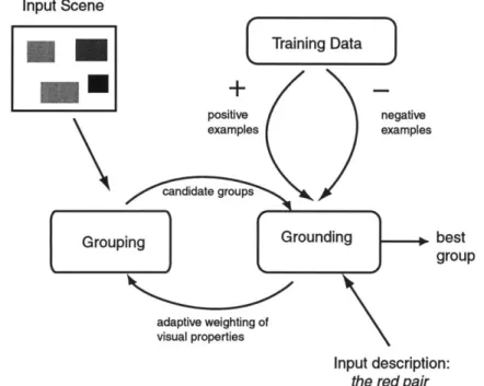
The diagram shown in Figure 1-1 shows our entire model. It can be divided into two stages. The first stage, indicated by the Grouping block, performs grouping on visual scenes. It takes a visual scene segmented into block objects as input, and creates a space of possible salient groups, labeled candidate groups, arising from the scene. We use a weighted sum strategy to integrate the influence of different visual properties such as, color and proximity. This stage also assigns a saliency score to each group. In the second stage, visual ground-ing, denoted in the figure by the Grounding block, the space of salient groups, which is the output of the previous stage, is taken as input along with a linguistic scene description. The visual grounding stage comes up with the best match between a linguistic description and a set of objects. The parameters of this model are learned from positive and negative ex-amples that are derived from human judgement data collected from an experimental visual referent identification task.
1.4 Organization
In the next chapter, Chapter 2 we discuss relevant previous research related to percep-tual organization, visual perception, and systems that integrate language and vision. In Chapter 3 we describe in detail the visual grouping stage, including a description of our grouping algorithm and the saliency measure of a group. In Chapter 4 we describe how visual grounding is implemented. We give details of our feature selection, the data collec-tion task, and the training of our model. The chapter is concluded with a fully worked out example that takes the reader through the entire processing of our model, starting from a scene and a description to the identification of the correct referent. In Chapter 5 we give details of our evaluation task and the results we achieved. In Chapter 6 we conclude, and discuss directions of future research.
Input Scene Training Data positive negative examples examples tegrups g
IGrounding
best group adaptive weighting of visual properties Input description: the red pair1.5 Contributions
The contributions of this thesis are:* A computational model for grounding linguistic terms to gestalt perception
" A saliency measure for groups based on a hierarchical clustering framework, using a weighted distance function
" A framework for learning the weights used to combine the influence of each
individ-ual perceptindivid-ual property, from a visindivid-ual referent identification task.
" A program that takes as input a visual scene and a linguistic description, and identifies
Chapter 2
Background
Our aim is to create a system that connects language and gestalt perception. We want to apply it to the task of identifying referents in a visual scene, specified by a linguistic description. This research can be connected to two major areas of previous work. The first area is visual perception and perceptual organization and the second area is building systems that integrate linguistic and visual information.
2.1 Perceptual Organization
Perception involves simultaneous sensing and comprehension of a large number of stimuli. Yet, we do not see each stimulus as an individual input. Collections of stimuli are organized into groups that serve as cognitive handles for interpreting an agent's environment. As an example consider the visual scene shown in Figure 2-1. Majority of people would parse the scene as being composed of 3 sets of 2 dots, in other words 3 pairs rather than 6 individual dots. Asked to describe the scene, most observers are likely to say three pairs of dots. This example illustrates two facets of perceptual organization, (a) the grouping of stimuli e.g., visual stimuli, and (b) the usage of these groups by other cognitive abilities e.g., language. Wertheimer in his seminal paper [30] on perceptual organization coined the term Gestalt for readily perceptible salient groups of stimuli, wholes, to differentiate from the individ-ual stimulus, parts. He also postulated the following set of laws for forming groups from individual stimuli:
Figure 2-1: Three pairs of dots
" Proximity -two individually perceived stimuli that are close to each other are grouped together.
" Similarity - two stimuli that are similar along a perceptual dimension, tend to be grouped together.
" Common Fate - stimuli sharing a common direction of motion tend to be grouped together.
" Continuity - two stimuli that fit the path of an imaginary or discontinuous straight line or smooth curve tend to be grouped together.
" Closure -two stimuli are grouped together so as to interpret forms as complete. This is due to the tendency to complete contours and ignore gaps in figures.
" Figure ground separation -a set of stimuli appear as the figure (positive space), with a definite shape and border, while the rest appear as background (negative space).
" Goodness of form (Pragnanz) -a set of stimuli a will be perceived as a better group compared to another set of stimuli b if a is a more regular, ordered, stable and bal-anced group than b.
Though not stated as a separate rule, using a combination of these principles simultane-ously to visually parse a scene, is another important and as yet unresolved [31] element
of perceptual organization. Wertheimer further gave examples from visual and auditory perception to show the applicability of these principles across different modalities.
Previous work related to perceptual organization has focused on computational mod-eling of the laws of perceptual organization. This involves creating a mathematical model that given all the current stimuli as input, will return groups of stimuli as output. The groups should be the same as formed by human observers. In the case of visual stimuli this amounts to forming groups from elements perceived in a visual scene. The formation of these groups could use one or all of the rules listed above. Each law of perceptual organi-zation, in itself, has given rise to whole bodies of work of which we give a few examples here.
Zobrist & Thompson [33] presented a perceptual distance function for grouping that uses a weighted sum of individual property distances. We use a similar distance function, but have a different weight selection method that learns the probability of usage of specific weight combinations by training on human group selection data. This is discussed in detail in Section 3.3 and Section 4.2. Quantifying similarity, especially across different domains has been discussed by Tversky [27], and Shepherd [21], and has given rise to the set the-oretic and geometrical functions for similarity judgment. In our work we use geometrical functions. A comprehensive discussion on similiarity functions can also be found in Santini
& Jain [18].
For detecting curvilinear continuity, the concept of local saliency networks was intro-duced by Sha'shua & Ullman [20]. Curved shapes can be detected by defining a saliency operator over a chain of segments. Optimization over all possible chains using a dynamic programming method leads to the detection of salient curves. For the principle of figure-ground segmentation and object detection, work has been done by Lowe [14] to use visual grouping for object recognition, and by Shi & Malik [22] for scene segmentation using normalized-cuts. One of the first methods for quantifying goodness of a group, in infor-mation theoretic terms, was presented by Attneave [9]. This work quantified goodness of a group through a measure of the simplicity of the group (the smaller the description of a group in some encoding scheme, the simpler it is). Amir & Lindenbaum [1] introduced a domain independent method for quantifying grouping. It abstracts the set of all elements
into a fully connected graph, and uses a maximum likelihood framework to find the best partition of the graph into groups. Using perceptual organization principles in applications has been an area that has received relatively lesser attention. Saund [19] presents a system for deriving the visual semantics of graphics such as sketches using perceptual organiza-tion. Carson et. al. [5] present another example in which gestalt grouping analysis is used as part of an image query system.
The references listed above tackle identifying salient groups as a purely visual problem, and try to model characteristics of low level human vision. In this thesis we wish to present work that uses not only visual, but linguistic information as well, to identify salient groups. We however, abstract the grouping problem to a higher level, where object segmentation of a scene is given, and the problem is to combine objects into groups that are referred to in the scene description.
2.2
Language and Perception
Research in the field of language and perception attempts to identify how what we perceive is affected by linguistic context, and how word meaning is related to perceptual input. The close link between language and perception has been studied [cf. 29] and modeled [cf. 15] in the past Special attention has been devoted to research on computationally modeling the relation between language and visual perception. It involves work related to building sys-tems that use visual information to create language descriptions, language descriptions to create visual representations or systems that simultaneously deal with visual and linguistic
input [23].
In our work we are primarily interested in investigating how the semantics of lan-guage can be derived through visually grounding linguistic terms. The problem of building grounded natural language systems using visual context, has been addressed in previous work such as the work done by [12], [10], [17] and [16]. The VITRA system [121 is a system for automatic generation of natural language descriptions for recognized trajecto-ries of objects in a real world image sequence such as traffic scenes, and soccer matches. In VITRA verbal descriptions are connected to visual and geometric information extracted
from the real-world visual scenes.
Gorniak & Roy [10] describes a system, Bishop, that understands natural language de-scriptions of visual scenes through visual grounding of word meanings and compositional parsing of input descriptions. It also provides a list of different strategies used by human subjects in a scene description task. In this list of strategies grouping is stated as an impor-tant but not fully resolved (in the paper) part. We have attempted to extend this work by specifically tackling the problem of understanding scene descriptions in which grouping is used as a descriptive strategy.
Roy [17] presents DESCRIBER, a spoken language generation system that is trained on synthetic visual scenes paired with natural language descriptions. In this work, word semantics are acquired by grounding a word to the visual features of the object being de-scribed. There is no a priori classification of words into word classes and their corre-sponding visual features, rather the relevant features for a word class, and the word classes themselves are acquired. The system further goes on to generate natural and unambiguous descriptions of objects in novel scenes. We have used a similar word learning framework as [17]. Work done by Regier [16] provides an example of learning grounded representation of linguistic spatial terms.
The main point of difference in our work is the handling of conceptual aggregate terms. Most language understanding systems handle linguistic input that refers to a single object, e.g., the blue block. We attempt to extend this work by trying to handle sentences like, the
group of blue blocks, or the blue stuff using a visually grounded model.
How language connects with perception has been studied extensively in the fields of psychology, and linguistics as well. The connection of language and spatial cognition and how language structures space was discussed by Talmy [24]. In it he stated that language schematizes space, selecting certain aspects of a referent scene, while disregarding others. Tversky [28] discusses the reverse relation of how space structures language. She presents an analysis of the language used in a route description task with an emphasis on discovering spatial features that are included or omitted in a description. These analyses support the notion of a bi-directional link between language and vision. Landau and Jackendoff [13] explore how language encodes objects and spatial relationships and present a theory of
spatial cognition. They further show commonalities between parsing in the visual system and language.
2.3 Initial Approaches
In this section we discuss, in brief, our initial approaches, and the insights we gained that led us to define and solve our final problem. As mentioned previously in Section 1.2, the initial motivation for tackling the problem of grouping was from the perspective of build-ing an application for document navigation and description. As we envisage the document description program, it will visually parse a given scene and then generate a natural lan-guage description of the scene, or read out information from a referent specified through a language description.
Documents can be handled by abstracting them to scenes composed of blocks encom-passing each letter and image. In this abstract form the problem resolves to finding salient groups in the document that correspond to how a reader might segment the document. The ideal segmentation would result in a set of groups at different levels of detail. At the low-est level letters will cluster to form words, and at the highlow-est level paragraphs will cluster to form articles, or sentences will cluster to form lists. The descriptor programi should perform the following four steps:
1. Segmentation
2. Grouping
3. Scene Hierarchy
4. Natural Language Generation
Of these four steps we worked on the first two, segmentation and grouping in web
pages. 1
A document discussing such a system can be found at
2.3.1 Segmentation of web pages
To analyze a document from the visual perspective it must first be segmented into atomic units that form the lowest level of the document hierarchy. This lowest level could be the pixel level, or even the letter level, depending on context. Thus, segmentation involves clus-tering at multiple levels of detail. The web pages were captured as images and converted to black and white. Run length smoothing followed by connected component analysis [6] was used to create bounding boxes for entities in a document e.g., letters and images.
2.3.2 Grouping
We implemented four different grouping/clustering algorithms. The first algorithm by Tho-risson [25] was used only on hand segmented images. The other three were used on images that went through the segmentation process detailed above. The three algorithms were (a) K-means, (b) Gaussian Mixture Modeling, and (c) Hierarchical clustering. Each took the block segmented document image as input and returned salient groups.
2.3.3 Discussion on initial approaches
Some of the issues that arose in our initial experimentation were:
" The need for a robust definition of similarity. Within the domain of input that we
considered, black and white block segmented images, simple proximity between the centroid of two blocks was sufficient. But, for colored images with a greater variety in shape and size, this would not suffice. Hence, there was a need to define a dis-tance function that combined the disdis-tances along various perceptual properties e.g., proximity, color, size, and shape.
" Multiple levels of grouping. The level of grouping is dependent on context, especially
linguistic context. The level decides the granularity of the elements to be grouped e.g., pixels, or objects. With this condition in mind, hierarchical clustering stood out as the best method.
* The language used for visual description. In describing web page images the lan-guage used is composed of higher level terms such as articles and lists. These terms are domain specific higher level examples of words whose semantics imply a con-ceptual aggregate. This adds a further layer of complexity to the problem. To avoid that, in our final framing of the problem, the input visual scene was simplified to a randomly generated synthetic scene made up of blocks. Note, as this was coupled with increasing the number of perceptual properties used in grouping there was a trade off in simplifying one aspect of the problem while complexifying another.
These issues helped define our final problem - building a model that looks at visual scenes composed of block objects having random location, size, and color, and trying to identify the correct referent based on a linguistic description. In the next chapter we present details of the gestalt grouping stage of our model.
Chapter 3
A model of Visual grouping
Visual grouping refers to performing perceptual grouping on a visual scene. It enables us to
see gestalts, i.e. create wholes from parts. In the grouping stage a visual scene is taken as
input and the output is a search space populated by groups that are perceptually observed on viewing the scene. In this chapter we frame the grouping problem as an unsupervised clas-sification (clustering) problem, discuss clustering algorithms, give reasons for our choice of using hierarchical clustering, and finally present the details of implementation.
3.1 Clustering algorithms
A visual scene can be viewed at different levels of granularity. At the most detailed level,
it is an array of pixels, and at the coarsest level it is composed of objects that compose the foreground, and the background. Grouping occurs at all levels. This is the reason why neighboring pixels combine to form objects, and why objects combine to form groups. The forming of groups in the visual domain can be mapped to the forming of conceptual aggregates in the language domain. For example, a group of birds can be referred to as a flock. Many other words in language such as, stuff used in the phrase -that stuff, pair used in
the phrase -a pair of, reveal semantics that classify such words as conceptual aggregates.
Thus, the first step towards connecting language and gestalt perception is to identify the groups in a visual scene that correspond to the conceptual aggregates in language.
selected an experimental task in which a visual scene is composed of rectangular objects
or blocks . The blocks are allowed to overlap. The problem of grouping can be stated as a
clustering problem. Here, the aim is to classify each object as belonging to a class ci from amongst a possible n classes. The value of n is unknown.
For modeling gestalt grouping we compared two specific classes of clustering algo-rithms Partitioning, and Agglomerative clustering [7]. Partitioning algoalgo-rithms tend to form disjoint clusters at only one level of detail. In contrast, Agglomerative algorithms e.g., hi-erarchical clustering attempt to classify datasets where there is a possibility of sub-clusters combining together to form larger clusters. Agglomerative algorithms thus provide
de-scriptions of the data at different levels of detail.
The ability to perform grouping on a scene at different levels of detail is similar to how our vision system does a multi-level parsing of a visual scene, as evident from the example of a group of birds being referred to as aflock. Due to this similarity hierarchical clustering was chosen. Another reason for our choice was the ability to define a goodness measure based on the hierarchical clustering algorithm that captures the gestalt property of stability
of a group. We discuss this measure in detail in section 3.6.
Before using hierarchical clustering a distance function between objects needs to be de-fined. The distance function should be such that, if distance(objecti, object2) < threshold, then objecti and object2 are grouped together. This criterion is related to similarity, be-cause in our context similarity is inversely proportional to distance. We formally define our distance function in the next section.
3.2 Perceptual Similarity
To group two objects together there must first be a quantification of how similar they are. We define the problem of quantifying similarity as one of calculating the distance between two objects in a feature space. Similarity can then be extracted as it is inversely proportional to distance. Conversely distance values can be treated as a measure of dissimilarity.
Each object o is defined as a point in a feature space, the dimensions of which are equal to the total number of perceptual properties. For example, the location of an object oi can
be represented by the object's x-coordinate (fi) and y-coordinate (f2) values, with respect to a fixed reference frame, as a vector,
[f
(3.1)More generally, the perceptual property of vector x of size I as,
x =
an object oi can be represented by a feature
(3.2)
We assume our feature space to be euclidean, hence the distance between two objects is given by,
d(oi, o) = (ffn2
-n=1I
(3.3)
We have used features whose perceptual distances can be approximated well by a eu-clidean distance in the chosen feature space, and can be termed as metrics because they satisfy the minimality, symmetricity and triangle inequality conditions [27]. The euclidean assumption is invalid for some measurements of perceptual similarity [18], but in this work we do not lay any claim to the universality of our similarity functions beyond the specific domain.
Distance between two groups, denoted by gn and gm is defined as the minimum distance between any two objects from the two groups,
gn -{o1,02, ... ,ov}
d(gn, gm) = min{d(oi, of)}
gm -
(01,102,
... , ow} V i,jsuch
that oi E gn and of E gm(3.4) (3.5)
area P number of pixels covered by an object L lightness
a positive values indicate amounts of red and
color negative values indicate amounts of green b positive values indicate amounts of yellow and
negative values indicate amounts of blue
x (centroidx) proximity y (centroidy) h (height) shape b (width)
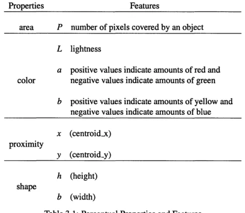
Table 3.1: Perceptual Properties and Features
3.2.1
Perceptual properties and Perceptual features
We wish to make a distinction here between perceptual properties and perceptual features. In language we refer to perceptual properties e.g., shape, that are physically grounded to perceptual features e.g., height and width. A perceptual property is calculated from perceptual features. Our discussion until now has dealt with defining the distance between two objects along only one perceptual property e.g., area, color etc. However, an object can be defined by more than one perceptual property. In our model we have currently included four perceptual properties -area, color proximity, shape. Table 3.1 lists the properties and
the features associated with each. The individual perceptual property distances are defined in the following sections.
Proximity
Given two objects oi and o, the contours of both objects are calculated. Let Ci and Cj be the set of all points belonging to the contours of oi and of respectively. The distance is
given by,
dp(oi,oj) = Vij,min{ (xi-xj)+(yi-yj) (3.7)
such that (xi,yi) E Ci and (x;,yj) E C;
Area
Given two objects oi and oj, all pixels corresponding to an object are counted. Assuming
oi has a Pi pixel size, and oj has a Pj pixel size,
da(Oi,Oj) = lPi-Pjl (3.8)
Color
For representing color we use the 1976 CIEL*a*b* feature space. This is a system adopted
by the CIE' as a model for showing uniform color spacing in its values. It is a device
independent, opponent color system, in which the euclidean distance between color stimuli is proportional to their difference as perceived by the human visual system [32]. The three axes represent lightness (L*), amounts of red along positive values and amounts of green along negative values (a*), amounts of yellow along positive values and amounts of blue along negative values (b*). The perceptual distance between any two colors can be found
by calculating the euclidean distance between any two points in L*a*b* space. Given two
objects oi and oj having color values, Li, ai, bi and Lj, a1, bj respectively the perceptual color distance can be stated as,
de(oi, oj) = (Li-L)2+ (ai - aj)2+(bi-b)2 (3.9)
The formula for conversion from rg,b space to CIEL*a*b* space is given in Appendix C.
Shape
The shape of an object is quantified by its height to width, i.e. aspect ratio. This measure can be calculated for arbitrary shapes by considering the bounding box of a given object. For object oi having height hi, width bi, and object of having height hj and width bj,
ds(oi,oj) =
lhi/bi-hj
1/bj (3.10)3.2.2
The combined distance function
The final distance function needs to combine the individual property distances. Our ap-proach to combining perceptual properties is using a weighted sum combination of the individual distances [33] for each perceptual property. The weight assigned to a percep-tual property is denoted by w and the the weights for all properties is denoted as a vector w. This approach assumes independence between perceptual properties. That is to say, area distance between two objects is independent of their color distance. In our model we measure area by calculating the number of pixels in the region covered by an object. This generalized method maintains the independence between area and shape, even though for rectangular objects area could be calculated using the height and width features that are
used for shape.
The final distance between two objects oi and o1, having P perceptual properties is
denoted by daiu (oi, oj) can thus be defined as,
di(oi, oj)
daui(oi, Oj) = [w1 ... wNI (3.11)
dp(oi, of) where,
In our case,
P = 4 (3.13)
di = dy, d2=da, d3=de, d4=ds (3.14)
3.3 Weight Selection
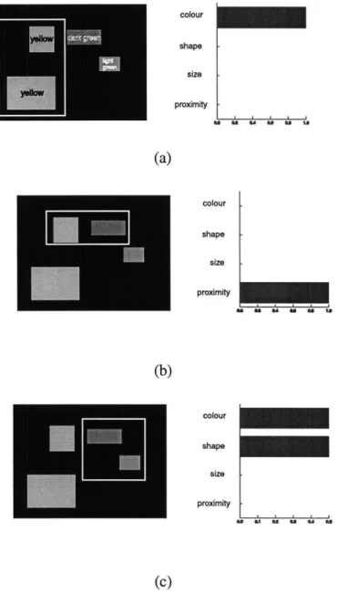
Selecting different weight values, for distance calculation, leads to different sets of group-ings. As an example, consider the visual scene in Figure 3-1.
The objects can be grouped together using area to give one set of groups or they can be grouped together using color to give another set. Further still, a combination of color and proximity effects could give yet another set of groups. A point to note here is that none of the resultant groupings are intuitively wrong. On a subjective basis one may be chosen over the other giving rise to a probability for each weight vector. A weight vector having a higher probability will give a more intuitive pop-out grouping in comparison to a weight vector with lower probability. We formulated a method to derive the probability values associated with each weight vector using data collected from a group selection task. For each group selected by a subject, in a particular visual scene, we calculated the weight vectors that would generate the same group from our grouping algorithm. For example, if a subject chose the selected group (shown by a white bounding box) in 3-1(a), then all weight vectors that gave the same grouping as output from the grouping algorithm would be recorded. The probability distribution over weight space is created using these recorded weight vectors. Thus, selecting which of the groups is best is similar to asking the question, which of the weight vectors used to form each group is the best.
3.3.1 Psychological basis
Triesman [26] conducted studies on referent search in visual scenes composed of objects that showed that search for a referent object in certain cases is parallel, hence very fast, while in other cases it is serial, and comparatively slower. Based on this evidence she put forward a visual model that created separate feature maps for salient features and
colour shape size mity colour shape size proximity Si I a lia colour shape size proximity a. at as as si as
Figure 3-1: Effect of different weight vectors on grouping
proxi
showed that the parallel searches correspond to searches in only one feature map, while serial searches correspond to searches through multiple feature maps.
Our notion of weights for each perceptual property is related to Triesman's feature maps. For example, if a scene referent is identified only on the basis of color, in Triesman's model this would correspond to a search in the color feature map, and in our model this would correspond to a group formed with color having a weight of 1, while all other prop-erties have a weight of zero. Thus, the most distinctive, pop-out group will correspond to weight vectors that have a non-zero value only for one of the properties color, or proximity, or area, or shape. This corresponds to the case where referent identification is done using a parallel search. The instance of a serial search is handled when the pop-out group cor-responds to a more complex weight vector similar to a combination of feature maps. We have expanded on the definition of a pop-out by trying to identify not just a single object, but rather a set of objects, i.e. a group pop-out.
3.4 Notation
Before presenting further details, we wish to familiarize the reader with the following no-tation which will be used here on. Some nono-tation used previously has been listed again as well, to provide a ready reference for all symbols used in the discussion to follow. Figure
3-2 contains visual examples of some of the notation presented here.
e o - an object in the visual scene
* 0 -
{
01, 02, ... , ON} set of all objects in a given scene* g -
{
01, 02, --- , on}
a group made up of one or more objects0 w -
{
wi, W2, ... , WI } a weight vector composed of weights for each perceptualproperty. All weight values lie between 0 and 1, and the sum of all weights wi is 1
g -
{
gi, g2, ... , g } a grouping made up of a set of groups created when weight vector is w, and threshold value is 00 GW -
{
g , g', ... , g'} a grouping hypothesis composed of one or more groupings.
Each weight vector w corresponds to a unique grouping hypothesis G* 7[ - {G"1, Gw2, ... , G""
}
the entire group space composed of all the grouping hypotheses generated from a specific visual scene3.5 Hierarchical Clustering
We have used a hierarchical clustering algorithm to generate groups in a visual scene. The choice of this algorithm was motivated by the need to generate groups at different levels of detail, and further to know the relationship between groups at each level. This means generating groups having few objects, when analyzing the scene in detail, or generating groups with a large set of objects, when analyzing the scene at a coarser level.
The grouping module takes 0 as input and returns n as output. The hierarchical group-ing algorithm for a given weight vector w is given in Figure 3-3.
The grouping model returns all possible groupings (composed of groups) over a range of weight vectors. We sample the value of each weight in the range [0,1], at intervals of 0.2 to come up with 56 different weight vectors. 56 weight vectors result in 56 group-ing hypotheses (GW), together forming the group space n. This is the input to the Visual grounding module.
The reason for carrying this ambiguity to the next stage is to be able to utilize linguistic information. This is an instance of our strategy to resolve ambiguities by delaying decisions until information from all modalities has been collected and analyzed.
3.6 Estimating pragnanz of a group
Starting from the seminal papers on Gestalt theory, one of the hardest qualities to define has been the goodness of a group. In traditional literature this is referred to by the term
pragnanz. Goodness of grouping gives a measure for ranking the set of all possible groups
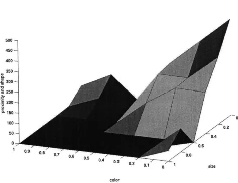
W1 901 W1 002 W1 093 GWi increasing threshold W2 901 W2 902 W2 g03 GW2
Figure 3-2: Stages of grouping for (a) weight vector w = [1 0] (proximity = 1, shape = 0),
variables
n < number of groups
8 < threshold increment
o
- thresholddistO <- distance function
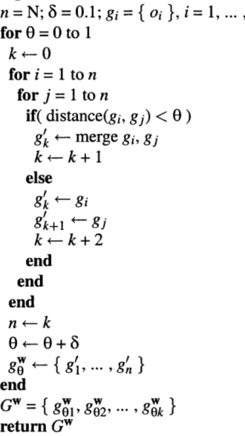
algorithm n = N; 8= 0.1;gi={o},i= 1,... , N; for 0=0 to 1 k <- 0 for i = 1 to n for j= 1 to n if( distance(gi, gj) < 0) g <- merge gi, gj k <- k + 1 else g <-- gi g'+1 <-- gj k <- k + 2 end end end n <-k 0 <- + 8 g90< g', ., g' } end G"= g, g"' g return GW
In our grouping algorithm a greedy approach is adopted, where the distance threshold value 0 is iteratively increased to initially allow formation of small groups until finally the threshold is large enough to allow all objects to fall into one group. The amount by which the threshold value has to change before any two groups merge to form a larger group is called the goodness/stability of the grouping. The formal definition is as follows.
Assume that for a fixed weight vector w, at a particular stage in the clustering process the distance threshold is 01 with an associated grouping g . Further assume, on incremen-tally increasing the threshold to 02 the corresponding grouping is g . If,
g = g (3.15)
g0 _ g (3.16)
g
#
(3.17)(3.18)
then,
goodness(g) = (02- 01)/sizeof(gw) where g E g (3.19)
the sizeofO function returns the total groups g in a grouping g'.
This value can be best described as measuring the gestalt property of stability, goodness,
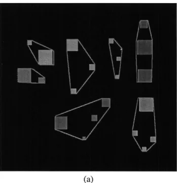
or pragnanz of a group. The figure 3-4 plots the formation of clusters versus the the
dis-tance threshold. The plateaus represent the points in grouping where changing the disdis-tance threshold did not result in the merging of any groups. This is the graphical representation of the goodness of a group. The adjoining image shows the grouping that corresponds to the longest, hence most stable plateau for number of clusters/groups equal to 7.
3.7 Summary
In this chapter we discussed the details of the grouping stage. The input to the grouping stage is a visual scene, composed of a set of block objects. The output, which is passed to
No. of groups vs. Threshold (w = [size = 0, color = 0.5, proximity = 0.5, shape = 0])
0.1 0.2 0.3 0.4
Distance threshold
(b)
the visual grounding stage, is the set of groups formed using all the weight vectors (7c), and a goodness of group/stability value corresponding to each group.
Chapter 4
Visual Grounding
We use the term grounding to mean deriving the semantics of linguistic terms by connecting a word, purely symbolic, to its perceptual correlates, purely non-symbolic [11]. Thus, the word red has its meaning embedded in color perception, as opposed to a dictionary, where red would be defined cyclically by other words (symbolic tokens).
The ability to form gestalts is a quality of human perception and in this chapter we present a methodology for grounding words to gestalt perception.
4.1 Word Learning
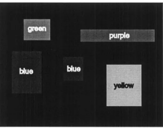
The problem we wish to solve is, given a novel scene and a description phrase, to accurately predict the most likely set of objects, i.e. a group, to which the phrase refers. An example of this is given in 4-1. Our solution involves training word conditional classification models on training pairs made up of a description and a group selection from a visual scene. As detailed in the following sections we first learn the semantics of individual words and then solve a joint optimization problem over all words in the input phrase to calculate a phrase conditional confidence value for each candidate group in the scene.
Figure 4-1: S: the green pair on the right
Word class Words Visual Features
grouping pair, group, stuff w (weight vector), N (number of objects in a group) spatial top, bottom, left, right x, y (location)
color red, blue, brown L, a, b
area large, small, tiny h (height), b (width)
Table 4.1: Word classes, words, and visual features
4.2 Feature Selection
In our model we deal with a limited vocabulary set that is divided a priori into four word classes. Through data collected from subjects in a visual selection task, we wish to ground each term in our lexicon to its appropriate set of visual features. Table 4.1 lists the word classes, their corresponding visual features, and example words belonging to each class. The full list can be also be seen in Appendix A.
Our prime focus is on connecting the meaning of words to features of a group. For this purpose, in the following section we define the group features that are connected to a word (belonging to the grouping word class) and present our method for extracting those features from collected data and the current visual scene.
Grouping terms
Visual grouping, in our model, occurs by clustering objects using a weight vector with each element of the vector specifying a weight over a perceptual property distance. Different groups can be generated using different weight vectors. We believe this weighting ability is part of gestalt perception. Thus, the true perceptual correlate to a grouping term is composed of (a) the size of the groups e.g., a pair implies a group of size 2, and (b) the combination of goodness of a group as defined in Section 3.6, and the weight vector. This is defined in section 4.5.1.
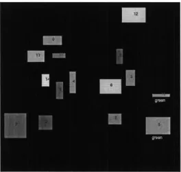
The size of a group, and the goodness of a group are calculated in the visual grouping module. Here we discuss how to calculate the probability of usage of a weight vector. We choose groups selected by subjects in our collected Dataset and correlate the group selec-tion with the weight combinaselec-tion that gives rise to the same group in our model. Figure 4-2 shows the probability of occurrence of a given weight combination in connection with a grouping selection. This surface has a maximum at proximity=1, color=O, area=O (only those cases where the weight for shape is zero were counted for the purpose of visualiza-tion).
This provides evidence for the general intuition that proximity dominates the groupings that we form. We interpret each point on this surface as the likelihood that a particular weight combination was used to perform a grouping.
4.2.1
The composite feature, from object properties to group
proper-ties
Averaging of group features is not a good method as the average along certain feature sets does not accurately represent the perceptual average of that set. For example, the average color of a group composed of a red, green, and blue object would be a fourth distinct color, which is perceptually wrong. What we really wish to do, is pool the word conditional likelihood of all objects that form a group. The method we employ calculates individual word conditional probabilities for each object and takes a logarithmic sum over those values. The logarithmic sum is equivalent to estimating the joint likelihood over all
Weight distribution 500-450 400 350 $00 -l .200 O 0-150-0.2 50 0.4 0. 1 0.9 0.8 0.7 0.6' 0.5 7 -0. 0. 0.4 0.3' 02sz color
Figure 4-2: Distribution over weight space
objects in a group, where the word-conditional probability of each object is independent of all other objects. Thus, given a word t, and a group g composed of objects oi, 02, On,
log[p(g1t)] = log[p(oil t)p(o2|t) ...p(onjt)) (4.1)
4.3 The data collection task
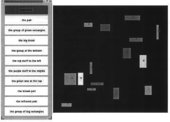
Data was collected in the form of pairs of linguistic descriptions and visual scenes. Subjects were shown two windows on a computer screen, as shown in 4-3.
One window displayed a visual scene composed of 15 rectangular objects, and the other window contained buttons to select description phrases. The properties of the objects in the visual scene e.g., area, position, color were randomly chosen and overlapping was allowed. The subjects were asked to select using a mouse, a phrase from the second window and all sets of objects that matched the phrase description from the first window. A new scene
button could be clicked to proceed to the next scene. Each selected object was highlighted
by a white boundary (the background color of all scenes was black). Deselection of an
object was allowed. The subjects were told to make a selection if they felt an appropriate set of objects existed in the scene, otherwise to make no selection at all. A no selection case was recorded when a phrase was selected but no objects were selected, or a phrase was not selected at all.
Figure 4-3: The data collection task
The phrases chosen for the task were constructed from words from our lexicon listed in Appendix A. Data was collected from 10 subjects, with each subject being shown a set of 10 phrases. The 10 phrases for each subject were chosen from a set of 48 unique phrases. Some phrases were shown to more than one subject. All the phrases can be seen in Appendix B. Along with the 10 phrases each subject was shown 20 different scenes, of which the first and last five were discarded, leaving 10 scenes, resulting in 100 phrase-scene pairs per subject. Aggregated over 10 subjects, this amounted to a total of 1000
unique phrase-scene pairs. As we use information from the no selection case to train our model, we have counted those cases as well. In the initial data collection it was noticed that there were insufficient exemplars for color terms, hence a 11th subject was used to collect data, but only for color description phrases e.g., the brown one. The selection of the number of objects in the scene (15) was done with an aim to elicit complex grouping choices. Appendix B contains a listing of all the phrases used according to subjects along with a histogram of word-class occurrence.
4.4 Grounding a word to its visual features
The collected data is composed of phrases and group selections. Each word in a description phrase is paired with the visual features of the objects in the corresponding group selection. Which visual features to associate with a word is based on the word class to which the word belongs. Formally, a phrase Sk is composed of words ti, and is paired with a group selection
gk from scene I. Each word ti is associated with a visual feature vector x that is dependent on the word-class of ti. We wish to estimate a distribution over all examples of a word and the corresponding selection. This in essence is a distribution estimated over all the good examples of a word. For example, an object selected as red would be a good example of
red, while one that is not selected as red would be a bad example of red. Thus we refer to
the values estimated over all good examples as the positive model parameters for a given word. We use the maximum likelihood estimates of the Gaussian parameters to estimate a word-conditional distribution over the feature space corresponding to the semantics of the word ti:
xx
k,wieSk j,ojEgk (4.2)
k,tiESk j,ojEgk
Oti = i (4.4)
For each word in our lexicon we also estimate a word-conditional distribution over all
bad exemplars associated with a word. For example, in a scene where a subject chose a
particular object as red, all other objects are classified as bad examples of a red object. The parameters of this distribution are referred to as the background model. Objects with features having a high probability value in the background distribution would qualify as
good examples of an object that could be described as not red.
IXj
k,tiESk j,Ojigk (45)
k,tiESk j,oj$gk
IT = E[(x-p)(x-Wp)4]
0 g = 0(4.6)
4.5
Selecting the best group, using good exemplars and
bad exemplars
The decision on how well a word describes a group of objects is based on calculating two confidence values:
1. Confidence that a group of objects is a good exemplar for a word ti,
2. Confidence that a group of objects is a bad exemplar for a word ti.
Figure 4-4: Detecting the absence of a red object
we will be forced to make an incorrect decision by choosing the object that has the highest rank, when sorted by confidence score. This raises the question of how to make a decision on the validity of the final answer given by our model. In the case shown in the figure, our model should be able to judge that an object is not red. Rather than building in a hard threshold value, we employ the information gained from the background model for a given word. Thus judging the validity of a group given a word can be framed as a two class classification problem, where the classes are good exemplars given ti, and bad exemplars given ti.
Once we have established the validity of a group, we rank the groups using the confi-dence value that it is a good exemplar for a given word. Our final answer for a group that corresponds to a given word will be the valid group that has the highest confidence value for being a good exemplar for the given word.
The validity of a group is based on satisfying the condition,
P(Kilot,) > P(gilo-t) (4.7) where,
p(gilt,) = N(p,,,t) (4.8)
Selecting the final answer can be formally stated as,
g = argmax p(gilot.) Vi, gi E I and gi is valid (4.10)
i
4.5.1
The case of grouping terms
Recall from section 3.3 that each group formed can be a member of multiple groupings, each of which is associated with a goodness measure, and a weight vector. The corre-sponding weight vectors are used to create a distribution over weight space that gives the probability of a given weight vector being used to form a selected group, labeled a good group, the parameters of which are labeled 6,, where ti is a word belonging to the grouping word class. We also estimate a distribution over weight space of the probability of a given weight vector not being used to form a selected group, the parameters of which constitute the background model and are labeled O6-.
We now combine the information from the positive and the negative examples to bias our final decision. Let w be the weight vector that corresponds to a grouping g" of which group g is a part. The group g must satisfy the following conditions:
p(g|1Ot) > p(gkIOti) Vk gk E , g 5 gk (4.11)
p(g|Ot) > p(gI6) (4.12)
As defined in the Chapter 3, n is the entire search space of all possible groups returned from the visual grouping module. We can calculate p(g|Ot) and p(g|6j-) as follows,
56 p(g|0ti) = p(g|6tiWp(wilot,) (4.13) i:=1 56 p(gIo7) = A p( iWp(wilog) (4.14) i=1
![Figure 3-2: Stages of grouping for (a) weight vector w = [1 0] (proximity = 1, shape = 0), and (b) weight vector w = [0 1] (proximity = 0, shape = 1)](https://thumb-eu.123doks.com/thumbv2/123doknet/14438203.516432/41.918.126.788.156.1016/figure-stages-grouping-weight-vector-proximity-weight-proximity.webp)