HAL Id: hal-02640519
https://hal.archives-ouvertes.fr/hal-02640519
Submitted on 28 May 2020
HAL is a multi-disciplinary open access
archive for the deposit and dissemination of
sci-entific research documents, whether they are
pub-lished or not. The documents may come from
teaching and research institutions in France or
L’archive ouverte pluridisciplinaire HAL, est
destinée au dépôt et à la diffusion de documents
scientifiques de niveau recherche, publiés ou non,
émanant des établissements d’enseignement et de
recherche français ou étrangers, des laboratoires
Sliding motion of a bubble against an inclined wall from
moderate to high bubble Reynolds number
Christophe Barbosa, Dominique Legendre, Roberto Zenith
To cite this version:
Christophe Barbosa, Dominique Legendre, Roberto Zenith. Sliding motion of a bubble against an
inclined wall from moderate to high bubble Reynolds number. Physical Review Fluids, American
Physical Society, 2019, 4 (4), pp.043602. �10.1103/PhysRevFluids.4.043602�. �hal-02640519�
OATAO is an open access repository that collects the work of Toulouse
researchers and makes it freely available over the web where possible
Any correspondence concerning this service should be sent
This is a publisher’s version published in:
http://oatao.univ-toulouse.fr/25
930
To cite this version:
Barbosa, Christophe
and Legendre, Dominique
and
Zenith, Roberto Sliding motion of a bubble against an inclined
wall from moderate to high bubble Reynolds number.
(2019)
Physical Review Fluids, 4 (4). 043602. ISSN 2469-990X.
Official URL:
Sliding motion of a bubble against an inclined wall from moderate
to high bubble Reynolds number
C. Barbosa,1,2D. Legendre,3and R. Zenit1
1Instituto de Investigaciones en Materiales, Universidad Nacional Autónoma de México,
Apartado Postal 70-360, México Distrito Federal 04510, Mexico
2Institut de Mécanique des Fluides de Toulouse (IMFT), Université de Toulouse,
CNRS-INPT-UPS, Toulouse, France
3Institut de Mécanique des Fluides de Toulouse (IMFT), Université de Toulouse, CNRS, Toulouse, France (Received 23 October 2018; published 26 April 2019)
The motion of a bubble sliding over an inclined wall from moderate to high bubble Reynolds number is studied experimentally for a wide range of liquid properties and bubbles sizes, considering wall inclination angles from nearly horizontal to nearly vertical. All experiments are restricted to sliding behavior, below the transition to steady bouncing motion. We study both the shape of the bubble and its drag coefficient. For small angles, the bubble shape is dominated by gravitational effects resulting in a flattened shape against the wall; for large angles, the bubble remains in constant contact with the wall but adopts a shape that is aligned perpendicularly to the wall, closer to that observed for an inertia-dominated free rising bubble. We model this transition of shape considering balances among surface tension, gravitational, and inertial forces; we observe good agreement with experiments. We found that the drag coefficient is strongly influenced by the shape that the bubble adopts as it slides over the wall. By considering the flow in the film and around the bubble, we propose a correlation to predict the drag coefficient for each regime of bubble shape. In the regime dominated by viscous effects, the drag of a single bubble is increased due to the mirror effect with the wall and by the friction in the film formed between the wall; conversely, for the case dominated by inertial effects, the drag coefficient is constant. The behavior for a single bubble is changed: no significant increase due to deformation. In both shape regimes the proposed expression agrees well with the experimental measurements.
DOI:10.1103/PhysRevFluids.4.043602
I. INTRODUCTION
Two phase flows are present in many natural phenomena and practical applications. For the case of dispersed gas-liquid flows, or bubbly flows, a good understanding of the overall dynamics has been reached [1]. Such progress is mainly supported by the knowledge of the motion of single bubbles and hydrodynamic interactions in unbounded fluids [2]. One of the remaining challenges in the understanding of these flows is the effect of walls. Although most flows are contained within walls, their effect on the bubble motion is still a subject of active research. For the particular case of bubbles, most studies have addressed the interaction of single bubbles with either vertical [3–6] or horizontal walls [7–9]. The interaction of a bubble with an inclined wall has been shown to be more complex: a bubble of a certain size and moving in a certain liquid may interact with the wall in a significantly different manner depending on the inclination. For small angles, the bubbles slide over the wall at a constant speed; for large inclinations, instead, the bubbles bounce repeatedly at a constant average speed. This phenomenon was first reported by Tsao and Koch [10]. The conditions for transition were recently explained by Barbosa et al. [11]: when the inertia
of the motion is sufficiently large, the wake behind the bubble induces a wall-repulsive lift force that pushes the bubble away from the wall. In the present paper we focus only on the sliding regime.
There have been several investigations that address the sliding motion of a bubble over an inclined wall, both experimentally [10,12–17] and by numerical simulations [16,18–20]. In particular, what is most relevant for practical applications is the determination of the drag coefficient of the bubble as it slides over the wall and the extent of contact with the wall. Both of these quantities can be used, for instance, to calculate the amount of heat and mass transfer that a bubble may extract from a heated wall [21].
Maxworthy [12] conducted experiments of sliding bubbles over an inclined plane but focused mostly on large bubbles, which in free rise state would have a spherical-cap shape (large Bond numbers, Bo= ρgDeq/σ, where ρ and σ are the density and surface tension, respectively, and g and Deq are gravitational acceleration and the diameter of the bubble, respectively). Conversely, Maslyiah et al. [13] and Tsao and Koch [10] conducted experiments for nearly spherical bubbles (small Weber numbers, We= ρU deq/σ, where U is the bubble speed) sliding on an inclined plane. They both proposed empirical correlations for the drag coefficient. In the investigation by Aussillous and Quéré [14], experiments were conducted for bubbles in highly viscous fluids and with very small angles of inclination. In this regime, a formal modeling of the flow was possible. They calculated the viscous lubrication force in the film between the bubble and the wall. An implicit formula for the capillary number (Ca= µU/σ , where µ is the liquid viscosity) is obtained from the force balance between the drag force and the buoyancy. Hodges et al. [22] studied the same configuration but for the case of droplets. Podvin et al. [16] conducted both numerical simulations and experiments to study the same system. They analyzed, in detail, the initial process of bubble-wall interaction. The existing numerical studies have focused on different aspects of the problem, covering the change of shape with inclination and Bond number [18], the shape and dynamics of large Bond number bubbles [19], and the change of shape with inclination [20]. The recent study by Dubois et al. [17] showed that the bubble shape could be aligned with the wall or be perpendicular to it depending on both the angle and the values of the Weber and Bond numbers. This behavior was captured in the numerical results of Senthilkumar et al. [20]. Dubois et al. [17] proposed a model based on a balance equation among buoyancy drag and the viscous resistance due to the film between the bubble and the wall.
In this article we report the experimental results of bubble sliding over an inclined wall. We cover a wide range of parameters by considering different fluids and bubble sizes. In particular, the bubble wall Reynolds number based on bubble diameter is varying from 10 to 650. The analysis of both the bubble shape and speed allowed us to separate the behavior of the sliding bubble into two distinct regimes: when the bubble shape is aligned with the wall and when the bubble is nearly perpendicular to it. Due to this significant change in the way the bubble moves on the wall, the resulting drag law is different. We propose drag correlations for each regime, based on the relevant forces for each case. The propose drag law depends on the Reynolds number, as expected, but it also includes lubrication effects, accounted for by the Bond and capillary numbers.
II. EXPERIMENTAL SETUP A. Methods and experimental conditions
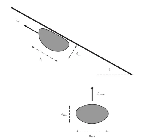
Figure1shows the bubble-wall interaction considered in this study: a bubble rising at terminal conditions interacts with an inclined solid wall. The experimental device is described in detail in [11]. In essence, it is a container in which an inclined wall is inserted. The angle of inclination of the wall can be varied from 5◦ to 80◦. The motion of the bubble during the interaction is captured using a high speed camera (Phantom v1) at a rate of at least 1000 frames/s, with a spatial resolution of 11.5 µm/pixel.
Vterm Vw dmi dma θ d d⊥
FIG. 1. Sketch of bubble terminal and wall conditions. Away from the wall, the bubble ascends at Vterm, with a constant aspect ratio dma/dmi, where dmaand dmimeasure the major and minor axis of the bubble. While sliding on the wall, the bubble moves at a constant speed, Vw, with an aspect ratio d∥/d⊥, where d∥ and d⊥
measure the bubble length and width with respect to the wall.
The bubble shape was determined by directly measuring the major and minor bubble axes dma and dmi, respectively, from each image. The equivalent diameter, Deq, is then calculated as
Deq= !
dma2 dmi "1/3
. (1)
The bubble aspect ratio was calculated from
χ =dma
dmi
. (2)
The terminal velocity, Vterm, is determined from the displacement of the bubble geometric centroid of consecutive frames, considering a central difference scheme. To calculate mean and standard deviations values of the measurements, each experiment was repeated five times. The uncertainty in the measurement of the bubble size and velocity is about 8%.
To generate a range of experimental conditions, seven different liquids and two capillary sizes were used. The physical parameters of the corresponding liquids as well as the terminal conditions for all cases are summarized in TableI. Note that we use the nomenclature in the first column of the table when referring to a specific case. The same symbols for each experiment are used in all the figures. The viscosity and surface tension of the different liquids were measured with a stress controlled rheometer (MCR101) and a Wilhelmy balance with a DuNouy ring, respectively. The density was measured with a 25 µL pycnometer. We characterize each experiment (a combination of bubble size with the physical properties of the liquid used) through the terminal Reynolds and
T ABLE I. Physical properties for all the experiments conducted in this in v estigation. In all cases, the liquids were mixtures of w ater (W), glycerol (G), and triethanol amine (T); percentages in the second column are by weight. Three experiments were performed using silicon oil (SO). The type of trajectory for b ubbles before reaching the w all is sho wn in the first column: rectilinear (R) or oscillatory (O). Composition, ρ µ σ Deq Experiment % (kg / m 3) (mP a s) (mN / m) (mm) Mo Re term We term χθ trans
E1
,
(R) SO, 100 855 1.280 18.0 1.1 5 .32 × 10 − 9 138 ± 31 .8 ± 0 .05 1 .31 ± 0 .02 80 ◦E2
,
(R) SO, 100 855 1.280 18.0 1.2 5 .32 × 10 − 9 172 ± 82 .6 ± 0 .17 1 .32 ± 0 .05 80 ◦E3
,
(O) SO, 100 855 1.280 18.0 2.2 5 .32 × 10 − 9 313 ± 74 .7 ± 0 .23 2 .06 ± 0 .04 45 ◦E4
,
(R) W -G, 80-20 1045 1.555 70.2 1.7 1 .59 × 10 − 10 305 ± 71 .9 ± 0 .09 1 .26 ± 0 .04 70 ◦E5
(6
),
(O) W -T , 99.88-0.12 1001 1.529 61.3 2.8 1 .15 × 10 − 9 250 ± 92 .0 ± 0 .11 1 .16 ± 0 .02 70 ◦E6
,
(O) W -G, 85-15 1033 1.363 70.0 1.6 9 .56 × 10 − 11 367 ± 16 2 .1 ± 0 .16 1 .44 ± 0 .05 65 ◦E7
,
(O) W -G, 90-10 1021 1.165 70.6 1.6 5 .03 × 10 − 11 469 ± 14 2 .5 ± 0 .15 1 .63 ± 0 .08 60 ◦E8
,
(O) W -G, 95-5 1009 1.038 70.8 1.7 3 .18 × 10 − 11 536 ± 21 2 .6 ± 0 .20 1 .58 ± 0 .07 60 ◦E9
,
(O) W -G, 90-10 1021 1.165 70.6 2.9 5 .03 × 10 − 11 640 ± 77 2 .6 ± 0 .51 .69 ± 0 .28 50 ◦E1
0
,•
(O) W , 100 998 0.955 72.6 1.6 2 .18 × 10 − 11 601 ± 40 2 .7 ± 0 .31 .78 ± 0 .10 50 ◦E1
1
,
(O) W , 100 998 0.955 72.6 3.1 2 .18 × 10 − 11 955 ± 46 3 .6 ± 0 .31 .93 ± 0 .13 45 ◦Weber numbers: Reterm= ρVtermDeq µ , Weterm= ρV2 termDeq σ , (3)
where Vtermis the bubble terminal velocity. The Morton number, defined as
Mo= gµ 4
ρσ3, (4)
is a dimensionless group that only contains fluid properties, so it is often used to characterize the fluid. Its value, for each liquid, is also reported in TableI.
When the bubble collides with the wall (always at its terminal velocity), it experiences few transient bounces and then achieves a new time-average steady state. As reported previously [10,11], the bubble can either slide steadily or bounce periodically with a constant mean tangential velocity. The conditions to observe one behavior or the other are discussed by Barbosa et al. [11]. They found that for wall angles below a certain critical value, θ < θtrans, the buoyancy force dominates the repulsive lift induced by the wake and the bubble slides under the wall; when θ > θtransthe lift induced by the wake is strong enough to push the bubble away from the wall and to generate a stable periodic bouncing. In this investigation we only consider bubbles that slide steadily on the wall after the initial wall interaction. Hence, for each bubble-fluid combination only the experiments for inclinations below the critical angle, θ < θtrans, are considered. To characterize the sliding steady state, wall Reynolds and wall Weber numbers are defined using the mean sliding velocity, Vw:
Rew= ρVwDeq µ , Wew= ρV2 wDeq σ . (5)
For the range of experimental conditions, the bubbles slide in a rectilinear manner over the wall. Maxworthy [12], for instance, did observe zigzagging for Bond numbers larger than 10.
B. Terminal conditions
The terminal conditions can be used to assess the degree of bubble deformation and surface contamination for each experiment. As shown below, these two effects determine the velocity of the bubble as it slides over the wall. According to the shape map proposed by Clift et al. [23], the range of experimental conditions studied here corresponds to ellipsoidal and wobbling bubbles with rectilinear and zigzag paths.
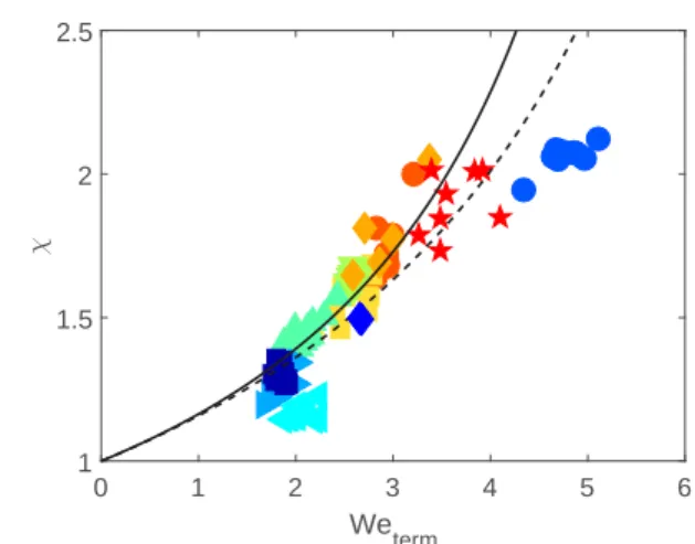
The evolution of the terminal aspect ratio with the terminal Weber number for the entire range of experimental conditions considered in this investigation is presented in Fig.2. The measurements are compared with the expression proposed by Legendre et al. [24]:
χ = 1
1−649Weterm(1+ K(Mo) Weterm)−1
, (6)
where Wetermand Mo are the Weber and Morton numbers. For this expression K (Mo)= 0.2 Mo1/10. The prediction of Eq. (6) is plotted for two cases. First, the prediction without the Morton number correction (χ = 1 + 9Weterm/64) is shown by the continuous line; the dashed line shows the prediction corresponding to Mo= 2 × 10⁻¹¹.
In general, the experiments agree well with the prediction. For large values of the Weber number, cases E3 and E11, Eq. (6) overestimates the experimental values. In these two data sets wobbling bubbles are observed; such motion affects measurement of the aspect ratio. For case E5, the experimental measurements are below the prediction of Eq. (6). For this particular experiment the liquid is strongly contaminated (this is shown below), as it contains a small amount of triethanol amine which is a long surfactant-like molecule. We can argue that in this case the surface contamination would alter the shape.
We term 0 1 2 3 4 5 6 χ 1 1.5 2 2.5
FIG. 2. Aspect ratio, χ , as a function of terminal Weber number, for all the experiments. Each bubble-fluid combination is represented by a different symbol, according to TableI. The continuous and dashed lines correspond to Eq. (6) plotted without the Morton term and for Mo= 2.1 × 10⁻¹¹, respectively.
Now, considering the value of the drag coefficient we can further assess the effects of bubble de-formation and the possible presence of surface impurities. The experimental steady drag coefficient is inferred indirectly from the balance between the buoyancy force and the drag force acting on the bubble in the vertical direction:
CD= 4 3 Deqg V2 term . (7)
The terminal drag is shown as a function of terminal Reynolds number for all the experiments conducted in this investigation in Fig.3.
Reterm
102 103
C D
10-1 100
FIG. 3. Drag coefficient, CD, as a function of terminal Reynolds number, Reterm, for all the experiments in Table I. The continuous black line shows the prediction of Eq. (9). The other continuous lines show the predictions of Eq. (10) for four cases: blue line, for Mo= 5.32 × 10⁻⁹ (E1, E2, E3); cyan line, for
Mo= 1.15 × 10⁻⁹(E5); green line, for Mo= 5.03 × 10⁻¹¹(E7, E9); and red line, for Mo= 2.18 × 10⁻¹¹
(E10, E11). The colors correspond to the nomenclature in Table I. The dashed black line shows the drag calculated according to Eq. (11).
For a spherical bubble at large Reynolds numbers, Levich [25] calculated that the drag coefficient would be
CDLevich=
48
Re (8)
resulting from the total viscous dissipation through the velocity potential of irrotational flow. Considering the effect of the boundary layer, but retaining the spherical shape, Moore [26] found that CDMoore= 48 Re # 1−2.211 Re1/2 $ , (9)
which extended its validity to Re≈ 50.
By additionally considering that the bubble was an oblate spheroid, Moore [27] calculated the drag coefficient to be CDMoore ∗ = Re48G(χ ) # 1+H (χ ) Re1/2 + · · · $ , (10)
where G(χ ) and H (χ ) are functions of χ , the bubble aspect ratio. Note that the aspect ratio corresponds to that in the terminal state, as in Eq. (2).
If the experimental results are in agreement with the prediction in Eq. (10), we can argue that the increase in drag is the result of deformation. In Fig.3we show the prediction for a few selected cases. For cases E1, E7, and E11 the agreement is reasonable. Hence, in these cases, we can argue that the interfacial contamination is not significant. On the other hand, the comparison between the prediction and the measurements for case E5 are significantly different. The experimental drag is well above the prediction, despite the fact that the bubble is not largely deformed (χ= 1.16). In fact, for this particular experiment the drag coefficient is close to that calculated for a fully contaminated surface (a solid sphere), according to the prediction by Schiller and Naumann [28]:
CDSN=
24
Re[1+ 0.15Re
0.687]. (11)
Therefore, as discussed above, for this particular experiment we consider that the bubble surface is immobile, resulting from surface active contaminants.
III. RESULTS
We now examine the motion and shape of bubbles as they slide on the wall. We show that the shape that the bubble adopts during its interaction with the wall strongly affects the drag and, therefore, the bubble speed.
A. Bubble shape on the wall
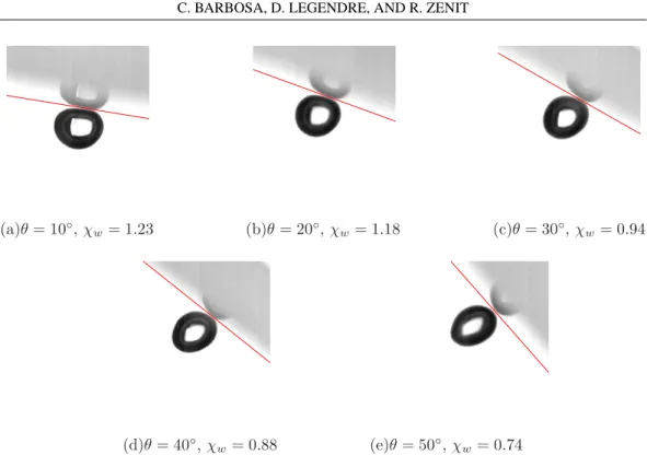
The shape of the bubble as it slides on the wall can be significantly different from that at its terminal condition. Furthermore, it can change importantly depending on the angle of inclination of the wall. Figure4shows sliding bubbles for different inclination angles for experiment E3. For small angles, Figs.4(a)and4(b), the bubble moves slowly and its shape is the result of the action of buoyancy pushing it against the wall. In other words, the bubble is elongated along the wall. For large wall inclinations, Figs.4(d)and4(e), the component of buoyant force that pushes the bubble against the wall is smaller. At the same time, the component of buoyancy in the direction parallel to the wall is larger resulting in a higher bubble velocity. In turn, the larger bubble velocity induces a deformation due to inertial effects similar to that observed under terminal conditions. Therefore, for these large angles, the bubble appears to be “standing” over the wall: its elongation is in the direction perpendicular to the wall. Clearly, for an intermediate inclination the bubble slides with a nearly spherical shape. Observations of the transition in bubble shape as the wall inclination increases
(a)θ = 10◦, χw= 1.23 (b)θ = 20◦, χw = 1.18 (c)θ = 30◦, χw= 0.94
(d)θ = 40◦, χ
w= 0.88 (e)θ = 50◦, χw = 0.74
FIG. 4. Images for the sliding bubble shape evolution at different inclination angles in experimental conditions E3 (see TableI): (a) Vw= 40.1 mm/s, Rew= 59, Wew= 0.04; (b) Vw= 80.9 mm/s, Rew= 119,
Wew= 0.16; (c) Vw= 115.0 mm/s, Rew= 169, Wew= 0.33; (d) Vw= 138.8 mm/s, Rew= 204, Wew=
0.48; (e) Vw= 155.2 mm/s, Rew= 228, Wew= 0.60. Images are shown with the same scale.
were recently reported by Dubois et al. [17]. They showed that the shape transition depends on both Weber and Bond numbers.
Therefore, we propose to use a different measure of bubble deformation when it interacts with the wall. The wall aspect ratio is defined as
χw=
d∥
d⊥, (12)
where d∥ and d⊥ are the bubble length parallel and normal to the wall, respectively. Therefore, for deformation controlled by gravity χw>1, whereas χw<1 is observed when deformation is
controlled by inertia. Below, we propose a model that considers the combination of these two effects to predict the bubble shape at the wall.
As observed, for a nearly horizontal wall, the bubble is pushed over the wall by the buoyant force and deformation is expected to be mainly controlled by gravity and the shape can be determined following Mahadevan and Pomeau [29], who considered the motion of a droplet rolling over a slightly inclined wall. In an analogous manner, we can consider that the bubble is nearly spherical everywhere except at the contact region, a flat horizontal disk of radius ℓ. By geometrical considerations, the vertical displacement of the bubble center δ due to the buoyancy and the radius of the contact disk ℓ are related to each other by ℓ2∼ Rδ, where R is the equivalent radius. The bubble deformation induces an increase of the bubble surface area by an amount 'a∼ ℓ4/R2and an increase of its radius 'R∼ ℓ4/R3. For the interaction with an inclined wall, the component of gravity acting towards the wall is g cos θ . Thus, balancing the decrease in potential energy ρg cos θ R3δ with the gain in interfacial energy σ 'a, the following scalings can be deduced: δ∼ Bo cos θR, ℓ ∼ Bo1/2cos1/2θR, and 'R∼ Bo2cos2θR. Therefore, the wall aspect ratio can
Bo cos(θ) 0 0.5 1 1.5 2 2.5 χ w 0.7 0.8 0.9 1 1.1 1.2 1.3 1.4 (a) Wew 0 0.5 1 1.5 2 2.5 3 χ w 0.5 1 1.5 (b)
FIG. 5. Dependence of wall aspect ratio for gravitational and inertial effects for all the experiments. (a) Wall aspect ratio, χw, as a function of Bo cos θ . (b) The wall aspect ratio, χw, as a function of the wall Weber
number, Wew. The symbols correspond to TableI: open and solid symbols represent experiments for χw>1
and χw<1, respectively. then be estimated to be χw= d∥ d⊥ ∼ 2R+ 2'R 2R+ 'R − δ ∼ 1 1− αBo cos θ, (13)
where α is a fitting constant. As shown by this relation, gravity flattens the bubble towards the wall. Note that this prediction is expected to only agree with measurements with small values of Bo cos θ . In Fig.5(a)the wall aspect ratio is shown as a function of Bo cos θ . Note that the data are shown according to their χwvalue: for χw>1 solid symbols are used, while open symbols are used when
χw<1. Clearly, for all liquids the value of χwdoes increase with Bo cos θ . However, the data do
not collapse into a single band of values including for χw>1 corresponding to deformation mainly
induced by gravity; hence, Bo cos θ is not the only parameter that determines the change of shape. When the wall inclination is large, closer to vertical, the bubble shape seems to be close to that observed for a free rising case as shown in Fig.4. For such a case, the bubble deformation is the result of the balance between inertial and surface tension forces. For freely ascending bubbles Moore [30] proposed a method to calculate the bubble deformation. Assuming that the bubble shape
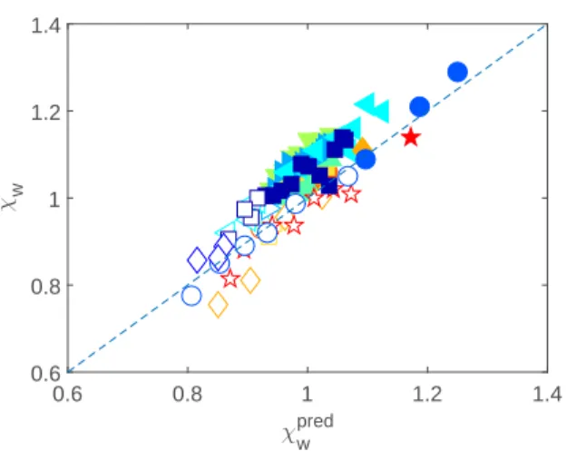
χwpred 0.6 0.8 1 1.2 1.4 χ w 0.6 0.8 1 1.2 1.4
FIG. 6. Comparison between the experimental value of χwand the prediction of Eq. (15), considering
α= 0.1 and β = 3/32, for all experiments in TableI: open and solid symbols represent experiments for χw>1
and χw<1, respectively. The dashed line shows the perfect correlation.
is an ellipsoid of revolution one can write d⊥ = 2R(1 − η/2) and d∥= 2R(1 + η), with η ≪ 1. By balancing the pressure distribution (from the irrotational flow around the bubble) with the surface tension force, it can be shown that η= −3/32We. For a bubble moving over a nearly vertical wall, considering Wewinstead of We, the wall aspect ratio can be expected to vary as
χw= d∥ d⊥ ∼ 1− βWew 1+β2Wew (14)
with β = 3/64 for a freely ascending bubble. This expression would only be able to predict the bubble shape for inclinations near the vertical value, corresponding to large values of Wew. The
effect of the interaction with the wall could be calculated by considering a mirror bubble. The potential solution of the velocity disturbance due to the mirror bubble is Vw(1+162s), where
s= Deq/L, taking L as the distance between the bubble center and the wall [31]. Considering that the bubble is in contact with the wall at s= 0.5, the velocity involved in the pressure at the bubble surface needs to be corrected by the prefactor 1+ 1/16 = 17/16. Therefore, the corrected value of the β coefficient would be βc= β(1716)
2
. This correction would result in a slight increase in the bubble deformation, of about 10%. For simplicity, we do not account for this effect. Therefore, in Fig. 5(b), we plot χw as a function of the corresponding Wew for all the experiments. As
expected, the deformation (in the direction perpendicular to the wall) increases with Wew. However,
considered alone the Weber number is not able to make possible a simple description of the bubble deformation when χw<1.
Both the gravitational and inertial effects on the bubble deformation need to be considered together to predict the wall aspect ratio. We now consider that a bubble deformed by gravity under the wall is also deformed by inertia due to its sliding motion. Combining both effects, the aspect ratio appears now under the form
χw=
(1− βWew)
(1− αBo cos θ )!1+β2Wew
" , (15)
where β= 3/32 and α can be determined experimentally. Figure6 shows the measured χw as a
function of the prediction from Eq. (15) considering a value of α= 0.1, obtained from a minimum square fit scheme of the data and the prediction. The prediction that takes into account both gravitational and inertial effects provides a much better correlation than those tested above. Note
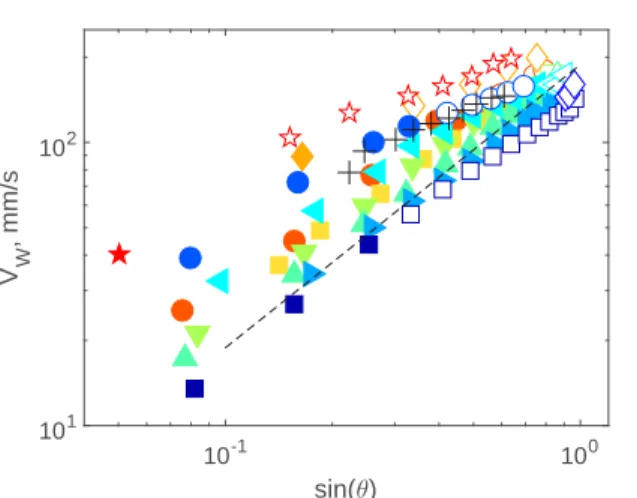
sin(θ) 10-1 100 V W , mm/s 101 102
FIG. 7. Sliding bubble velocities, Vw, as a function of sin θ , where θ is the inclination of the wall, for all
the experimental conditions of TableI. The black+ symbols show the results of Dubois et al. [17] for water (Deq= 2.0 mm). The dashed line shows the trend of the experiments by Tsao and Koch [10] (Deq= 1.6 mm), also for water.
that from Eq. (15) it is possible to determine the values of Wewand Bo for the transition, considering
that χw≈ 1.
B. Sliding velocity and wall drag coefficient
The evolution of the steady sliding velocity with the inclination angle is shown in Fig.7for all the experimental conditions of TableI. For all experimental conditions, the bubble-wall velocity increases monotonically with the inclination angle. For all cases, the bubble velocity increases with wall inclination angle. When χw>1, the wall velocity appears to increase linearly with sin θ ; when
the shape is such that χw<1, the increase of velocity with wall inclination is less pronounced.
Clearly, the value of the velocity depends on both the size of the bubble and the properties of the liquid. As shown, the trend for the velocity is found to be in good agreement with previous experimental results [10,17].
To analyze the dynamic behavior of the motion, we need to determine the hydrodynamic force on the bubble as it slides over the wall. The driving force is simply the buoyancy, corrected for the wall inclination. The drag force parallel to the wall balances the buoyancy, and the corresponding balance equation can be written in terms of a wall drag coefficient such that
CDw= 4 3 Deqg sin θ V2 w . (16)
Considering the classical representation, Fig. 8shows the drag coefficient, CDw, as a function of the wall Reynolds number, Rew, defined above, for all experimental conditions. As in the previous
figure, the experimental values of CDware shown as solid or open symbols for χw>1 or χw<1,
respectively. For the case of χw>1 (bubbles elongated along the wall) a general trend of the form
CDw∼ Re−1w is observed in accordance to what is observed for freely rising bubbles. Note that the drag coefficient does not fall into a single band of data, indicating that significant additional effects have to be accounted for. For bubbles with χw<1 (bubbles elongated in the direction perpendicular
to the wall), the drag coefficient appears to reach a constant value with respect to Rew.
1. Wall drag coefficient for χw> 1
For freely rising spherical bubbles, the drag coefficient can be described by Moore’s expression, Eq. (9), for Re > 50. However, for Re < 50, this expression is no longer applicable and it displays
Re w 101 102 103 C Dw 10-1 100 101
FIG. 8. Wall drag coefficient CD w, as a function of wall Reynolds number, Rew, for all the experimental
conditions of TableI. The solid and open symbols show the experiments for χw>1 and χw<1, respectively.
The black continuous and dashed lines show the prediction of Eqs. (17) and (20), respectively.
a nonphysical behavior. Instead we can use the expression proposed by Mei et al. [32] (obtained by fitting direct numerical simulations in order to recover Eq. (9) when Re→ ∞):
CDMei = 48 Re[1+ F (Re)] (17) where F (Re)= − 2.211Re 1/2 + 32/3 Re+ 3.315Re1/2+ 16. (18)
The function F (Re) could be interpreted as the drag correction that accounts for a spherical bubble boundary layer and wake whatever the value of Re. This relation is shown by the black continuous line in Fig. 8, considering Vw instead of Vterm, to calculate CDw and Rew. It serves as a reference
to be contrasted with the wall measurements. As expected, the prediction is below that found for all experiments because the effect of the additional drag induced by the presence of the wall is not accounted for. Nevertheless, for the case of bubbles with χw>1, the decreasing trend of the drag
coefficient also follows a Re−1dominating trend.
When a bubble moves near a wall we can consider two additional contributions to the drag. First, the mirror image of the bubble induces a drag increase [33] which is at first order,
CDw=
48 Rew
(1+ s3), (19)
where s= Deq/L, L being the distance between the bubble center and the wall. For a spherical
bubble in contact with the wall s= 0.5. The second mechanism for drag increase is due to the production of additional vorticity on the bubble surface induced by the proximity of the wall. Figueroa et al. [6] showed that the additional drag due to vorticity production was 6s3C
DMoorefor
a bubble moving in between two walls. Therefore, considering the effect of only one wall and superposing the mirror effect, we can expect an evolution of the form
CDw= 48
Rew
(1+ 4s3+ F (Rew)), (20)
where F (Rew) is defined by Eq. (18) and the term in s3 accounts for the mirror effect and the
additional vorticity production. This prediction, considering a value of s= 0.5, shown in Fig.8 by the black dashed line, is now closer to the experimental results for the E1 case. For this case,
the bubbles are nearly spherical (with a maximum Wew= 1.26). The rest of the experiments have
larger values of the drag coefficient than the prediction. Equation (20) was derived to consider two effects in interaction with a vertical wall: the mirror image of the bubble and the vorticity production at the wall. Although the prediction gives a better estimate of the wall drag, it is still below the experimentally obtained value for most cases. The fact that the predicted drag can be brought closer to the experimental measurements is noteworthy, but it is clear that the formulation is not sufficient to quantitatively calculate the wall drag. It is important to note that the flow analyzed by Figueroa
et al. [6], from which Eq. (20) was derived, is not exactly the same as that studied here, since a film between the bubble and the wall is formed by the action of gravity. As shown before, this contribution needs to be accounted for in the description of the deformation; it is thus expected to have an effect on the drag force. Below, we directly consider the effect of the film between the bubble and the wall on the total wall drag.
When the bubble slides over the wall a flattened region appears and a thin lubrication film causes an increase of the drag force. The deformed region can be determined by a balance between gravitational and surface tension forces, as discussed by Mahadevan and Pomeau [29] for a horizontal wall and by Hodges et al. [22] for small inclination. Extending these results to an inclined wall (Bo being replaced by Bo cos θ ) the size of the contact region can be shown to be
ℓ∼ (Bo cos θ )1/2Deq for Bo cos θ < 1, (21)
ℓ∼ (Bo cos θ )1/4Deq for Bo cos θ > 1. (22)
The film thickness is obtained by considering the deformation induced by the viscous motion and the viscous effect in it [14]. The resulting film frictional viscous force is
Ffilm∼ σ ℓ Ca2/3w , (23)
where Caw= Vwµ/σ is the wall capillary number. Writing the film force in dimensionless terms,
we have
CDfilm∼ 1
Rew
(Bo cos θ )n
Ca1/3w , (24)
where n= 1/2 for Bo < 1 and n = 1/4 for Bo > 1.
Now, assuming that the effects can be superposed, we can write an expression for the drag on the bubble that accounts for the potential interaction and the viscous film drag. The mirror-additional vorticity contribution (6s3C
DMoore) is now replaced by the film drag [Eq. (24)] and we have
CDw= 48 Rew % 1+ s3+ F (Rew)+ Ko (Bo cos(θ )n Ca1/3w & , (25)
where Kois a constant that needs to be determined from the experiments.
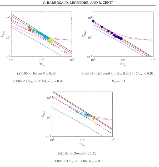
To compare the experimental measurements with the prediction of Eq. (25) we separate the experimental results depending on whether Bo cos θ < 1 or Bo cos θ > 1. Figure 9(a) shows experimental results for the case when Bo cos(θ ) < 1. For this group of experiments the Bond number is approximately the same with a maximum value of Bo cos(θ )= 0.38. The continuous and dashed lines in the plot show the prediction of Eq. (25) considering n= 1/2 and two values of the wall capillary number, corresponding to the minimum (continuous line) and maximum (dashed line) values of Caw: the black lines show the predictions for a small angle (θ = 5◦), while the red
lines show the predictions for a large angle (θ = 74◦). The prediction, considering Ko= 0.3 as
the only fitting coefficient, agrees well with the experimental measurements. To show the relative importance of the viscous film term, the blue dash-dotted line in the figure shows the drag coefficient with Ko= 0.0 (i.e., neglecting the film drag). For this case, the film friction accounts for up to 75%
of the total drag; the mirror-image drag is approximately 5% of the total drag. Note also that the influence of the inclination angle is small.
Re w 101 102 103 C Dw 10-1 100 101 (a)0.05 < Bo cos θ < 0.40, 0.0003 < Caw< 0.004, Ko= 0.3 Re w 101 102 103 C Dw 10-1 100 101 (b)0.09 < Bo cos θ < 0.61, 0.001 < Caw< 0.01, Ko= 0.1 Re w 101 102 103 CDw 10-1 100 101 (c)1.00 < Bo cos θ < 1.56, 0.0005 < Caw< 0.006, Ko= 0.3
FIG. 9. Comparison between the measured wall coefficient and the prediction of Eq. (25). The continuous and dashed lines are the predictions for minimum and maximum values of Caw, respectively; the black lines
show the prediction for θ = 5◦; the red lines show the prediction for θ= 74◦, corresponding to the minimum
and maximum angles of the entire set. (a) Bo < 1, n= 1/2, experiments E4, E6, E7, E8, and E10; (b) Bo = 0.58, n= 1/2, experiment E1; and (c) Bo > 1, n = 1/4, experiments E5, E9, and E11. In all cases the blue dash-dotted line shows the prediction of Eq. (25) without the film drag (Ko= 0.0). The magenta lines show the
prediction from the model of Dubois et al. [17] for the corresponding values of the capillary numbers.
Of all the experiments with Bo cos θ < 1, only one case did not appear to be well predicted by Eq. (25) considering Ko= 0.3. This case is shown in Fig.9(b), which corresponds to experiment
E1. For this case, the bubbles are nearly spherical and the fluid is silicon oil which can be considered free of surface active agents. Considering that in this case we can expect a complete slip of the fluid velocity on the bubble surface, the drag on the film would be smaller than in the case of a partially contaminated bubble. Therefore, we can argue that for this particular experiment the value of the fitting coefficient Kowould be smaller. The lines on the plot were obtained considering Ko= 0.1.
The Bond number is 0.57 and Ca= 0.01 or Ca = 0.001. The agreement is also very good. In this case, the film drag accounts for only roughly 40% of the total drag.
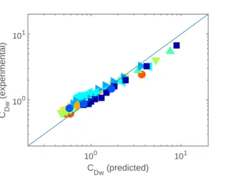
C Dw (predicted) 100 101 C Dw (experimental) 100 101
FIG. 10. Comparison between the experimental drag coefficient and the predictions from Eq. (25). The line shows a perfect correlation.
Figure 9(c) shows the experimental results for Bo cos θ > 1, for which n= 1/4. For these experiments, the functional dependence of CDwchanges, according to Eq. (25). Considering a range
of values of Bo cos θ from 1 to 1.56, the minimum and maximum values of Cawand Ko= 0.3, the
prediction of the drag agrees well with the experimental measurements. The film drag for this case is about 70% of the total amount. Note also that the value of Kois the same as for the data shown in
Fig.9(a), despite the fact that the Bond number is different.
For clarity we now show the predictions of Eq. (25) as a function of the experimentally determined drag coefficient, for all the experiments conducted in this investigation. The comparison is shown in Fig. 10. Clearly, the predictions are in good agreement with the experimental measurements. The maximum difference between the prediction and the experiments is about 30%. We can now draw some comparisons with previous models. From Dubois et al. [17], we can obtain an expression for the total wall drag coefficient, given by
CDw = α Re+ β + a 2 π ' 2 3 1 Re Bon Ca1/3 (26)
with n= 1/2 or n = 1/4 for Bo < 1 and Bo > 1, respectively. The parameters α = 16, β = 0.65, and a= 9 are fitting coefficients of their experiments conducted for 0.026 ! Rew! 840. The first
two terms correspond to the drag resulting from the flow around the bubble and the third term corresponds to the film drag. The coefficient α is much smaller that its equivalent term in Eq. (25) and corresponds to the small Reynolds limit of F (Re). The value of the coefficient β is discussed in the next section. For the film drag, the value a= 9 corresponds to Ko= 0.0975. This value is
significantly smaller than ours (Ko= 0.3). The predictions from Eq. (26) are shown in Fig.9, by
the magenta lines. Overall, the wall drag coefficient is underpredicted by this correlation for small Rew; the agreement is better for Bo > 1. There is a significant deviation of behavior for large values
of Rew.
It is also possible to draw comparisons with the model proposed by Aussillous and Quéré [14]. They addressed only the small Rewregime (Rew! 0.2 for their experiments) so their prediction is
not reported in our figures for clarity. Writing their force expression in the same format as Eq. (25), we have CDw= a 16 3 1 Re+ b 8 3 1 Re Bo1/2 Ca1/3, (27)
where a= 5 and b = 2.3 are fitting parameters. The value of a is larger than that for the viscous drag force of a single bubble (a= 3), in agreement with our Eq. (25). The fitting coefficient b can
Re w 101 102 103 C Dw 10-1 100 101
FIG. 11. Wall drag coefficient, CD w, as a function of wall Reynolds number, Rew, for all the experiments
from TableIfor which χw<1. The dash-dotted line shows CD w= 0.7. For comparison, the dashed line shows
the prediction from Eq. (20). The solid and dashed magenta lines show the predictions from Eq. (26) from Dubois et al. [17], for two different values of the capillary number.
compared to our Koin our Eq. (25), leading to Ko= b/18 = 0.128 which is in reasonable agreement
considering the differences in the range of Re.
2. Wall drag coefficient for χw< 1
As discussed above, when the bubble is deformed due to the inertia of the flow, the wall aspect ratio is smaller than one (χw<1). In this case, the bubble shape is closer to that observed in a
freely rising bubble. Barbosa et al. [11] argued that the drag force on such bubbles results from the pressure difference between the front and the rear of the bubble where the flow is detached so that the pressure difference scales as ρV2
w and we can expect that FD∼ ρVw2D2eq. For such a shape, the formation of “proper film” is not clear [see Figs.4(c),4(d), and4(e)]. The contact area between the bubble and the wall is very small; therefore, the induced dissipation in this region is not expected to result in a dominant contribution. In other words, the film drag gives negligible contribution. Considering that the drag force is balanced with the buoyancy, we have
ρVw2D2eq∼ ρgD3eqsin(θ ). (28)
Considering the definition of the drag coefficient, from Eq. (16), we can write
CDw ∼
gDeqsin(θ )
V2
w
= const. (29)
Therefore, if χw<1 the wall drag coefficient can be expected to be independent of the wall
Reynolds number. Note that the Froude number can be defined as Frw= Vw/
(
gDeq from which we can write Fr2
w∼ sin(θ ).
Figure11shows the drag coefficient as a function of the Reynolds number, for the data with χw<1, which clearly shows that CDw≈ 0.7 and nearly constant for most experiments. This value
is close to the fitting parameter β= 0.65 in Dubois et al. [17]. The data cover a significant range of wall Reynolds numbers from 150 to 650, approximately. The only case for which the experimental drag is not within the rest corresponds to experiment E5, which has been argued to have significant levels of surface contaminants; therefore, it could be expected to show larger values of the drag. Note that this change of trend was already reported by Tsao and Koch [10] but was not discussed
or identified. In the figure, the prediction from Eq. (26) is shown for two values of the capillary number. Clearly, for large Rewthe prediction asymptotes to a similar value.
IV. CONCLUSION
In this paper we studied the motion of bubbles sliding steadily over a flat inclined wall. Surprisingly, previous studies had not proposed a generalized correlation for the drag coefficient of the bubble in this configuration. More importantly, the alignment of the bubble with respect to the wall had not been identified as a relevant feature to determine such a coefficient. Thanks to the wide range of experimental parameters that were covered in the study, we were able to, first, identify the conditions for the transition between bubble alignment with the wall or perpendicular to it. Consequently, the experimental data were divided into two groups. In this manner, drag correlations were proposed for each case, taking into account only the relevant physical mechanisms involved in each condition. What our results show is that the transition from spherical to oblate shape that leads for a single bubble to a significant increase of the drag coefficient due to deformation (see Fig.5 in Maxworthy et al. [34] and our Fig.3) is not observed for a bubble moving in a close interaction with a wall. Indeed, the drag coefficient changes directly to a constant value corresponding an inertia dominating drag.
[1] F. Risso, Agitation, mixing, and transfers induced by bubbles,Annu. Rev. Fluid Mech. 50,25(2018). [2] J. Magnaudet and I. Eames, The motion of high-Reynolds-number bubbles in inhomogeneous flows,
Annu. Rev. Fluid Mech. 32,659(2000).
[3] F. Takemura and J. Magnaudet, The transverse force on clean and contaminated bubbles rising near a vertical wall at moderate Reynolds number,J. Fluid Mech. 495,235(2003).
[4] A. W. G. De Vries, A. Biesheuvel, and L. Van Wijngaarden, Notes on the path and wake of a gas bubble rising in pure water,J. Multiphase Flow 28,1823(2002).
[5] M. F. Moctezuma, R. Lima-Ochoterena, and R. Zenit, Velocity fluctuations resulting from the interaction of a bubble with a vertical wall,Phys. Fluids 17,098106(2005).
[6] B. Figueroa-Espinoza, R. Zenit, and D. Legendre, The effect of confinement on the motion of a single clean bubble,J. Fluid Mech. 616,419(2008).
[7] K. Malysa, M. Krasowska, and M. Krzan, Influence of surface active substances on bubble motion and collision with various interfaces,Adv. Colloid Interface Sci. 114–115,205(2005).
[8] R. Zenit and D. Legendre, The coefficient of restitution for air bubbles colliding against solid walls in viscous liquids,Phys. Fluids 21,083306(2009).
[9] E. Klaseboer, R. Manica, M. H. W. Hendrix, C. D. Ohl, and D. Y. C. Chan, A force balance model for the motion, impact, and bounce of bubbles,Phys. Fluids 26,092101(2014).
[10] H. K. Tsao and D. L. Koch, Observation of high Reynolds number bubbles interacting with a rigid wall,
Phys. Fluids 9,44(1997).
[11] C. Barbosa, D. Legendre, and R. Zenit, Conditions for the sliding-bouncing transition for the interaction of a bubble with an inclined wall,Phys. Rev. Fluids 1,032201(2016).
[12] T. Maxworthy, Bubble rise under an inclined plate,J. Fluid Mech. 229,659(1991).
[13] J. Maslyiah, R. Jauhari, and M. Gray, Drag coefficient for air bubbles rising along an inclined surface,
Chem. Eng. Sci. 49,1905(1994).
[14] P. Aussillous and D. Quéré, Bubbles creeping in a viscous liquid along a slightly inclined plane,
Europhys. Lett. 59,370(2002).
[15] A. Perron, L. I. Kiss, and S. Poncsak, An experimental investigation of the motion of single bubbles under a slightly inclined surface,Int. J. Multiphase Flow 32,606(2006).
[16] B. Podvin, S. Khoja, F. Moraga, and D. Attinger, Model and experimental visualizations of the interaction of a bubble with an inclined wall,Chem. Eng. Sci. 63,1914(2008).
[17] C. Dubois, A. Duchesne, and H. Caps, Between inertia and viscous effects: Sliding bubbles beneath an inclined plane,Europhys. Lett. 115,44001(2016).
[18] K. M. DeBisschop, M. J. Miksis, and D. M. Eckmann, Bubble rising in an inclined channel,Phys. Fluids
14,93(2002).
[19] C. E. Norman and M. J. Miksis, Dynamics of a gas bubble rising in an inclined channel at finite Reynolds number,Phys. Fluids 17,022102(2005).
[20] S. Senthilkumar, Y. M. C. Delaure, D. B. Murray, and B. Donnelly, The effect of the VOF-CSF static contact angle boundary condition on the dynamics of sliding and bouncing ellipsoidal bubbles, Int. J. Heat Fluid Flow 32,964(2011).
[21] B. Donnelly, T. S. O’Donovan, and D. B. Murray, Surface heat transfer due to sliding bubble motion,
Appl. Therm. Eng. 29,1319(2009).
[22] S. R. Hodges, O. E. Jensen, and J. M. Rallison, Sliding, slipping and rolling: the sedimentation of a viscous drop down a gently inclined plane,J. Fluid Mech. 512,95(2004).
[23] R. Clift, J. R. Grace, and M. E. Weber, Bubbles, Drops, and Particles (Academic Press, New York, 1978). [24] D. Legendre, R. Zenit, and J. R. Velez-Cordero, On the deformation of gas bubbles in liquids,Phys. Fluids
24,043303(2012).
[25] V. G. Levich, The motion of bubbles at high Reynolds numbers, Zh. Eksp. Teor. Fiz. 19, 18 (1949). [26] D. W. Moore, The boundary layer on a spherical gas bubble,J. Fluid Mech. 16,161(1963).
[27] D. W. Moore, The velocity of rise of distorted gas bubbles in a liquid of small viscosity,J. Fluid Mech.
23,749(1965).
[28] L. Schiller and A. Z. Naumann, A drag coefficient correlation, Z. Ver. Dtsch. Ing. 77, 318 (1933). [29] L. Mahadevan and Y. Pomeau, Rolling droplets,Phys. Fluids 11,2449(1999).
[30] D. W. Moore, The rise of a gas bubble in a viscous liquid,J. Fluid Mech. 6,113(1959).
[31] D. Legendre, J. Magnaudet, and G. Mougin, Hydrodynamic interactions between two spherical bubbles rising side by side in a viscous liquid,J. Fluid Mech. 497,133(2003).
[32] R. Mei, J. Klausner, and C. J. Lawrence, A note on the history force on a spherical bubble at finite Reynolds number,Phys. Fluids A 6,418(1994).
[33] J. B. W. Kok, Dynamics of a pair of gas bubbles moving through liquid. Part I. Theory, Eur. J. Mech. B
12, 515 (1993).
[34] T. Maxworthy, C. Gnann, M. Kurten, and F. Durst, Experiments on the rise of air bubbles in clean viscous liquid,J. Fluid Mech. 321,421(1996).