An energy approach describes spine equilibrium in adolescent idiopathic scoliosis

HAL Id: hal-03032969

https://hal.archives-ouvertes.fr/hal-03032969

Submitted on 1 Dec 2020

HAL is a multi-disciplinary open access archive for the deposit and dissemination of sci-entific research documents, whether they are pub-lished or not. The documents may come from teaching and research institutions in France or abroad, or from public or private research centers.

L’archive ouverte pluridisciplinaire HAL, est destinée au dépôt et à la diffusion de documents scientifiques de niveau recherche, publiés ou non, émanant des établissements d’enseignement et de recherche français ou étrangers, des laboratoires publics ou privés.

An energy approach describes spine equilibrium in

adolescent idiopathic scoliosis

Baptiste Brun-Cottan, Pauline Assemat, Vincent Doyeux, Franck Accadbled,

Jérôme Sales de Gauzy, Roxane Compagnon, Pascal Swider

To cite this version:

Baptiste Brun-Cottan, Pauline Assemat, Vincent Doyeux, Franck Accadbled, Jérôme Sales de Gauzy, et al.. An energy approach describes spine equilibrium in adolescent idiopathic scoliosis. Biomechanics and Modeling in Mechanobiology, Springer Verlag, 2020, 19 (5), pp.1-12. �10.1007/s10237-020-01390-9�. �hal-03032969�

OATAO is an open access repository that collects the work of Toulouse

researchers and makes it freely available over the web where possible

Any correspondence concerning this service should be sent

to the repository administrator:

tech-oatao@listes-diff.inp-toulouse.fr

This is an author’s version published in:

http://oatao.univ-toulouse.fr/26846

To cite this version:

Brun-Cottan, Baptiste and Assemat, Pauline and Doyeux,

Vincent and Accadbled, Franck and Sales de Gauzy, Jérôme

and Compagnon, Roxane and Swider, Pascal An energy

approach describes spine equilibrium in adolescent idiopathic

scoliosis. (2020) Biomechanics and Modeling in

Mechanobiology. ISSN 1617-7959.

Official URL:

https://doi.org/10.1007/s10237-020-01390-9

An energy approach describes spine equilibrium in adolescent

idiopathie scoliosis

Baptiste Brun-Cottan 18

·

Pauline Assemat1 _{• Vincent Doyeux}1 _{• Franck Accadbled}1_•2 _{• Jérôme Sales de Gauzy}1_•2 _•

Roxane Compagnon 1_•2 _{• Pascal Swider}1

Abstract

The adolescent idiopathie scoliosis (AIS) is a 3D deformity of the spine whose origin is unknown and clinical evolution unpredictable. In this work, a mixed theoretical and numerical approach based on energetic considerations is proposed to study the global spine deformations. The introduced mechanical model aims at overcoming the limitations of computational cost and high variability in physical parameters. The model is constituted of rigid vertebral bodies associated with 3D effec­tive stiffness tensors. The spine equilibrium is found using minimization methods of the mechanical total energy which circumvents forces and loading calculation. The values of the model parameters exhibited in the stiffness tensor are retrieved using a combination of clinical images post-processing and inverse algorithms implementation. Energy distribution patterns can then be evaluated at the global spine scale to investigate given time patient-specific features. To verify the reliability of the numerical methods, a simplified model of spine was implemented. The methodology was then applied to a clinical case of AIS (13-year-old girl, Lenke lA). Comparisons of the numerical spine geometry with clinical data equilibria showed numerical calculations were performed with great accuracy. The patient follow-up allowed us to highlight the energetic role of the apical and junctional zones of the deformed spine, the repercussion of sagittal bending in sacro-illiac junctions and the significant role of torsion with scoliosis aggravation. Tangible comparisons of output measures with clinical pathology knowledge provided a reliable basis for further use of those numerical developments in AIS classification, scoliosis evolution prediction and potentially surgical planning.

Keywords Global spine · Scoliosis · Mechanical model · Functional minimization · Inverse problem · Medical imaging

1 Introduction

The adolescent idiopathie scoliosis (AIS) is a multifacto­ rial disease potentially involving genetic, metabolic and mechanical aspects, and which affects up to 3% of the 10--16 years population with a significant female prevalence. AIS is characterized by the deviation of anatomical spine cur­ vature toward coupled 3D deformation involving abnormal bending and torsion. It generally shows a rapid evolution during the growth spurt (Riseborough and Wynne-Davies

1973) which can lead to respiratory and cardiac disorders.

igj Pascal Swider pascal.swider@imft.fr

2

Institut de Mécanique des Fluides de Toulouse, IMFT, CNRS, Université de Toulouse, Toulouse, France

Children Hospital, Toulouse University Hospital, Toulouse, France

If orthotic treatment fails to stop progression which happens in 10% of AIS, the surgery is indicated. Scoliosis clinical management might improve the early diagnosis, the predic­ tion of its unstable evolution and deterministic information for the surgical planning.

The proposed methodology concemed a mechanical approach to explore the equilibrium of adolescent scoliotic spines. The causality of the disease is not studied. In the literature, several modeling strategies have been proposed to predict the mechanical response of a scoliotic spine. In van der Plaats et al. (2007), the authors developed a numerical finite element model to test a buckling hypothesis as initia­ tion of the AIS. The results were descriptive and comparison with clinical data remained to be performed. Lafage et al. (2004) investigated an all spine model using adapted struc­ tural elements, but as pointed out by the authors, no physical model was developed to adjust the mechanical parameters used. Drevelle et al. (2010) proposed a 3D FEM model to

mimick AIS evolution, a study that was limited by the lack of follow-up to assess the clinical evolution of the spine. Despite significant progress in the anatomy characterization of AIS (Araújo et al. 2017) and previously cited modeling efforts, most of studies resulted in qualitative propositions for scoliosis description.

In particular, the 3D generic approach of FEM finds its limitation in the size of the problem and the lack of knowl-edge in tissue properties and boundary conditions in vivo (Ferguson et al. 2004; Jebaseelan et al. 2012). Alterna-tive discrete mechanical models of children spines involv-ing soft tissues and muscles have been proposed (Schmid et al. 2019). To examine the soft tissues and, especially the intervertebral disk (IVD) role into the AIS time course, studies at reduced scale have been proposed. For instance, Stokes (2007) focused on the biomechanical interaction between the IVD and the vertebral body in scoliosis evolu-tion. This hypothesis is supported by recent clinical studies which highlight the altered response of disk in AIS popula-tion (Abelin-Genevois et al. 2015; Langlais et al. 2018). The poromechanical response of vertebral segments was numeri-cally predicted using a dedicated substructuring technique to reduce computation costs (Swider et al. 2010). As soft tissues are structures with maximal energy gradients (Violas et al. 2007; Noailly et al. 2007; Swider et al. 2010), multiple studies focused more specifically on the IVD characteriza-tion. Information about effective mechanical properties of IVD (Newell et al. 2017) and some components of segment effective stiffness are available (Schultz et al. 1979; Stokes et al. 2002; Meng et al. 2015). However, these approaches involved ex vivo experimental measurements and none of them concerned the adolescent. Another strategy could be to identify in vivo properties at tissue scale (Jebaseelan et al.

2012; Langlais et al. 2018; O’Connell et al. 2007) but pedi-atric functional imaging are rarely available.

To address the lack of physical parameters availability and the numerical limitations, we aimed at developing a new mechanical and numerical model in order to characterize the overall scoliotic spine deformation. The progression of scoliosis is targeted after diagnosis and the cause of scoliosis initiation is not explored in this study. A 3D wired model that overcomes the previous limitations based on original key points was constructed. To achieve this modeling, it was hypothesized that the quasi-static evolution of scoliosis fol-lowed an energetic minimization law, and that an effective stiffness tensor which models deformable structure inter-acting at a vertebral segment scale existed. The values of this tensor were reconstructed based on clinical data using reverse analysis.

2 Materials and methods

In this section, we develop the wireframe model and detail the theoretical formulation based on energy minimization and numerical methods. This methodology is evaluated on a test case and applied to a clinical application on a 2 years follow-up of a 13-year-old scoliotic patient.

2.1 Parameterization of the vertebral segment

Parameterization of the spine is described in Fig. 1a, b associ-ated with EOS® _{exams used in the clinical application of}

para-graph 2.4.2. Vertebral bodies follow rigid body motions and by contrast, disks, vertebral endplates, facet joints, ligaments and other soft tissues connected with the vertebral segments are considered as deformable tissues. Figure 1c shows a model of vertebral segment Si including the deformable structure

between two rigid vertebral bodies, Vi and Vi+1.

To establish the kinematic description of the wireframe model, a unique orthonormal basis Bi was associated to each

vertebra i as shown in Fig. 1d. The vector 𝐞𝐱 i joined the

cent-ers Oi and O′i of vertebral endplates of the vertebra i. The

sec-ond vector 𝐞_{𝐲 i} was defined by the orientation of the spinous process. The vector 𝐞𝐳 i warranted the condition of a direct

orthonormal reference frame. A similar method defined Bi+1

attached to i + 1.

Considering now a vertebral segment, composed of two vertebrae (i and i + 1 ) and an IVD, the two reference frames of vertebra i were Ri(Oi, Bi) and Ri�(O_i�, B_i) , and the ones of

the vertebra i + 1 were Ri+1(Oi+1, Bi+1) and Ri�₊₁(O_i�₊₁, B_i+1).

The displacement continuity at the boundary of a vertebra and an IVD ensured the uniqueness of the points Oi , O′i and

led to the following linking equations for the local reference frames:

where 𝐑i was a rotation matrix, expressing the

orienta-tion of a base Bi+1 in Bi , and 𝐎i , 𝐎′i , 𝐎i+1 were the

vec-tor formed with the points Oi , O′i , Oi+1 and the point O0 .

Vector 𝐓i depended on the deformation of the IVD and 𝐋_i∕R

i = (lvi, 0, 0)

𝖳 , l

vi being the length of a vertebrae.

We considered that the matrix 𝐑i was the result of 3

succes-sive rotations of 3 angles noted 𝜃i, 𝛼i, 𝜑i (details in “Appendix

1”).

The kinematics of the vertebral body i + 1 was described, relative to i, in the reference frame Ri by the position vector 𝐮_i∕R

i involving the 6 components introduced in 𝐓i∕Ri and 𝐑i:

(1) 𝐎�_i− 𝐎i= 𝐋i, 𝐎i+1− 𝐎�i= 𝐓i, and B_i +1= 𝐑iBi, (2) 𝐮_i∕R i = (Txi, Tyi, Tzi, 𝜃i, 𝛼i, 𝜑i) 𝖳_.

The concatenation of vectors 𝐮i∕Ri , noted 𝐮∕Ri allowed the

kinematics of the whole spine to be obtained iteratively. To ease further developments and, especially manage-ment of spine boundary conditions and gravity loading (Sect. 2.2), the kinematic fields were also written into an absolute reference frame RA(OA, BA) . The unique

ortho-normal basis BA defined the frontal plane of the trunk in

anatomical position, with OA located at the top of the first

thoracic vertebra (T1). The basis Bi of each vertebra was

related to the global basis BA by:

In Eq. (3), 𝐏i was a unique rotation matrix resulting from

cumulative rotations of subjacent vertebral bodies k = 1 … i. (3) B_i= i ∏ k=1 𝐑_kB_{A= 𝐏i}B_{A, with} 𝐏_i= i ∏ k=1 𝐑_k.

Fig. 1 EOS® _{radiography of}

a female adolescent with pro-gressive scoliosis and param-eterization of the biomechanical wireframe model. a Frontal acquisition at age 13 (1A Lenke type and 40◦ Cobb angle) and

anatomical description of the spine, b frontal acquisition at age 15 ( 65◦ Cobb angle), c

schematic view and notations of a vertebral segment T9–T10, only frontal components are represented and vertical gravity is 𝐠 , d representation of a local reference frame associated with a vertebral body i

We had, in the global base BA , the expression of the

vec-tor 𝐋i:

We called 𝐗i∕RA the vector characterizing the displacement

of the IVD such that:

However, the position of the points Oi, Oi′ allowed us to only

know the location of each vertebral body. To keep track of the information concerning the orientation of the vertebrae (torsion), we also introduced 𝐘i∕RA:

For further use, we called 𝐮∕RA the concatenation of the

vec-tors 𝐗i∕RA and 𝐘i∕RA.

2.2 Governing equations of spine balance by minimization of total potential energy

The spine dynamics was studied in a time scale long enough to smooth daily variations and short enough to assume a closed and non dissipative system. Consequently, transient effects due to diffusion, convection, and structural damp-ing could be averaged in the studied time window 𝜏 dur-ing which all forces could be considered conservative. The model achieves an extraction of mechanical parameters from clinical data at the specific time of the X-ray image capture. No growth model has been integrated. For each different clinical data, i.e., time point, a new numerization is performed from which we can deduce the length of the vertebrae and of the IVD, although the IVD growth is very limited for the patient studied as she is older than 12. The first hypothesis was that the spine mechanical behavior could be described by a succession of quasi-static states, at equi-librium in 𝜏 . The second hypothesis was that the nonlinear mechanical response eventually due to nonlinear material properties, large displacements or large strains, could be searched in the form of successive piecewise linear equi-libria. This implied that associated forces derived from a local potential.

The total potential energy V was the sum of internal strain energy of the isolated segment generated by the strain of the deformable structure between one vertebra relatively to the adjacent one and the work of external loading taking into account the distributed body weight (gravity) and the role of muscles and ligaments. Components of vector 𝐮 were nondimensionalized by the height of thoracic and lumbar spine of the patient.

The segment displacement field 𝐪i was defined by the

difference between the kinematics 𝐮i and a reference energy

(4) 𝐋_i∕R A = lvi𝐏i⋅ 𝐞𝐱 i. (5) 𝐗_i∕R A= 𝐓i∕RA= 𝐏i⋅ 𝐓i∕Ri. (6) 𝐘_i∕R A= 𝐏i⋅ 𝐞𝐲 i state 𝐮0

i . The independent symmetric tensors 𝐊i ( 6 × 6 ) and 𝐁_i ( 6 × 6 ) were, respectively, associated with local strain

energy and potential energy of external mechanical forces. Therefore, the contribution of forces inside the vertebral segment and due to disk, muscles or any other tissue was included into the effective tensor 𝐊 . The contribution of forces outside the vertebral segment such as dorsal muscle, gravity, or other components such as braces, was included into the effective tensor 𝐁 . Vector 𝐆i ( 1 × 6 ) represented the

contribution of gravity forces. In the following, the variable

𝐩will correspond to the components of the effective tensors

( 𝐊 and 𝐁 ) and to the reference state 𝐮0 . The dependence of

the total potential energy V to 𝐮 and 𝐩 was defined as:

When considering energy from internal deformation of a vertebral segment, the displacement was expressed in local coordinates, with a relative unconstrained position of one vertebra to the adjacent one [Eq. (8)]. When considering the work of external forces, the description of the spine was developed in the absolute reference frame [Eq. (9)].

Using Eqs. (8) and (9), Eq. (7) became:

Kinematics boundary conditions were imposed at the lim-its of the region of interest. Locations and orientations of extremal vertebral bodies were obtained from X-ray clinical exams and used as input into the absolute reference frame.

2.3 Numerical resolution

2.3.1 Resolution of the direct problem

Knowing a set of parameters 𝐩 , the admissible stationary kinematic field 𝐮 which minimized V was called 𝐮eq(𝐩) and

described the static equilibrium of the system. The stability conditions were described as:

(7) V(𝐮, 𝐩) =∑ i 𝐪𝖳_i ⋅ 𝐊i⋅ 𝐪i+ ∑ i 𝐪𝖳 i ⋅ 𝐁i⋅ 𝐪i− ∑ i 𝐆_{i⋅ 𝐪i}. (8) 𝐪_i∕R i = 𝐮i∕Ri− 𝐮i 0 ∕Ri, (9) 𝐪_i∕R A= 𝐮i∕RA− 𝐮i 0 ∕RA. (10) V(𝐮, 𝐩) =∑ i 𝐪_i𝖳 ∕Ri⋅ 𝐊i⋅ 𝐪i∕Ri+ ∑ i 𝐪_i𝖳 ∕RA⋅ 𝐁i⋅ 𝐪i∕RA− ∑ i 𝐆_{i⋅ 𝐪i∕R} A.

The problem of minimum search was strongly nonlinear, and the surface response of the function V(., 𝐩) ∶ u ↦ V(𝐮, 𝐩) was non convex. Solutions were found by implementing a trust-region algorithm and a Newton algorithm [Scipy library, Virtanen et al. (2019)] sequentially to accelerate convergence. Gradient ∇𝐮V and hessian matrix ∇𝐮∇𝐮V were

also analytically calculated to minimize computation time.

2.3.2 Resolution of the inverse problem

For the clinical problem, we did not have access to mechan-ical tensors nor initial reference states. To identify the parameters and to test the robustness of our approach, we implemented an inverse problem methodology (Tarantola

2005). This was formulated by the set of Eqs. (12), (13) and (14) where 𝐮eq(𝐩) was the kinematic equilibrium, 𝐮c was the

observed clinical equilibrium (EOS® _{X-ray) and 𝐩}

sol was the

converged solution of mechanical parameters:

with ̄Kk,k the mean value defined as: ̄Kk,k= 1

m

∑

iKk,k,i and

m the number of vertebral segment. The formulation was

adapted to full effective tensors 𝐊 and 𝐁 . The problem size was reduced when clinical applications were considered and only diagonal terms of stiffness tensor 𝐊 were taken into account. Therefore, only those terms appeared in the penalty function c(𝐩) described by Eq. (14).

The objective function f involved the distance function d and the penalty function c. The distance function weighted the norm of discrepancies between predicted equilibrium

𝐮_eq(𝐩) and clinical data 𝐮_c . The direct problem resolution provided 𝐮eq(𝐩) at each incremental step. Matrix 𝐒 was used

to attenuate the impact of values with smaller precision from the clinical data (rotation of vertebrae). Penalty function

c(𝐩) aimed at deforming the image surface of the objective function f in order to give more weight to the set of param-eters minimizing the penalty function c. Mean values and

(11) 𝐮_eq(𝐩) = argmin 𝐮 (V(𝐮, 𝐩)). (12) 𝐩_sol = argmin 𝐩 ( f(𝐮_eq(𝐩), 𝐩)) with f(𝐮_eq(𝐩), 𝐩) = d(𝐮_eq(𝐩)) + c(𝐩), (13) d(𝐮_eq(𝐩)) = (𝐮_eq(𝐩) − 𝐮_c)𝖳 ⋅ 𝐒 ⋅ (𝐮eq(𝐩) − 𝐮c), (14) c(𝐩) = 𝜖₁ 6 � k=1 ( ̄K_k,k− K_prior k,k) 2₊ 𝜖₂ 6 � k=1 m � i=1 (Kk,k,i− ̄Kk,k)2+ 𝜖₃(‖𝐮0− 𝐮0_prior‖2),

variances of tensors coefficients were, respectively, penal-ized in first term and second term of equation (14) using prior values as controls.

The inverse problem was solved using a Newton con-jugate gradient algorithm (Scipy library) which required the first and second derivatives of the objective function f. The first derivation was obtained using the adjoint method detailed in “Appendix 2”. The second derivation was evalu-ated numerically using finite differences, exploiting the multi-core potential of the computer to fill the hessian matrix ∇_𝐩∇_𝐩f faster (linear acceleration).

The nondimensionalized difference aec of 𝐮eq and 𝐮c

expressed by Eq. (15) was an indicator of the methodology accuracy with a 0 value for a perfect fit.

Beyond the determination of the kinematic field, the meth-odology allowed us to determine the distribution patterns of energies using Eq. (7). The model proposed an energy method to circumvent the ignorance of forces, tissue prop-erties, detailed anatomy and local boundary conditions, by assuming the existence of energy local potentials. As a result, distribution patterns of energies were determined using Eq. (10). In addition, forces considered as model out-put measures, could be calculated using Eq. (16) in post-pro-cessing thanks to equilibrium 𝐮eq and effective parameters 𝐩

obtained from the inverse problem.

However, we will not work with forces distribution in the spine in the following and only the energetic approach will be exploited as it includes more information, it circumvents the lack of loading knowledge at the boundary conditions and it is the starting point of our model.

2.4 Applications

2.4.1 Numerical test case of a 34 elements simplified spine

The vertical wireframe model was made of 34 elements cor-responding to m = 17 vertebral bodies and deformable ele-ments as shown in Fig. 2a. Diagonal terms of 𝐊 were fixed to 1 and all other components were nil. The reference state was defined by 𝐮i0_∕R

i = (1, 0, 0, 0, 0, 0)

𝖳 , i = 1.17 in the local

reference frames. This set of parameters was called 𝐩ref in

the following parts. Boundary conditions in the absolute reference frame were 𝐮∕RA(1) = (0, 0, 0, 0, 0, 0)

𝖳 and

𝐮_∕R

A(17) = (25, 0, 0, 0, 0, 0)

𝖳.

We solved the direct problem and verified its conver-gence. We ran it multiple times to obtain many possible

(15)

a_ec = ‖𝐮eq− 𝐮c‖ ‖𝐮c‖

(16)

equilibrium positions. We then chose one of the equilibrium position, and used it as reference position 𝐮c for the test on

the inverse problem. We solved the inverse problem using this reference geometry and verified the convergence of the numerical solver first. Then we verified that the solution geometry 𝐮eq and 𝐮c were the same. Ultimately, we looked

for a correspondence between the solution parameters and the reference ones.

2.4.2 Clinical application

Clinical data were extracted from a clinic radiological pro-spective monocentric study approved by the Institutional Review Board of the Ethic Committee (Toulouse Univer-sity Hospital). Spine geometry in frontal and sagittal planes were obtained in vertical position by a low-dose X-ray EOS®

system. The rotation of vertebrae was calculated using the remoteness of the spinal process. The selected patient was

a 13-year-old girl diagnosed with a 1A scoliosis according to Lenke classification (Lenke et al. 2001) and a 40◦ Cobb

angle in 2014. The deformation progressed to 65◦ and ended

up to a T2–L2 surgical spinal fusion in 2016 (Fig. 1b for an illustration of Cobb angle).

A python® _{custom-made script was implemented in}

ImageJ® _{to build the wireframe description of the scoliotic}

spine from T1 to L5 and to build 𝐮c for 34 elements. The

boundary conditions were fixed in term of location and orientation in T1 and L5. The reference state was defined assuming an isotropic level dependent compression of deformable elements in standing position, i.e 𝐮0= 𝛼 × 𝐮c .

This approximation of 𝐮0 was based on the mean size

vari-ation of healthy patient between morning and night (Lude-scher et al. 2008; Zhu et al. 2015).

The terms of effective mechanical tensors 𝐊i and 𝐁i

were reduced to the diagonal terms and associated priors of Eq. (12) were adapted from the literature (Meng et al. 2015;

Fig. 2 Numerical test case with 34 wireframe elements mimick-ing a simplified adolescent spine: a wireframe schematic view, b four solutions 𝐮eq of

the direct problem, c conver-gence of the inverse problem in term of objective function and residual

Newell et al. 2017). The gravity loading Gi, followed the values introduced in Villemure et al. (2004). These choices still led to an inverse algorithm dealing with a size of 153 parameters. In this clinical application, the direct problem numerical resolution was starting close to uc contrary to the

simplified spine model in Sect. 2.4.1 which explored the multiplicity of solutions. This methodology, in addition to asymmetric boundary conditions, lead to the uniqueness of equilibrium geometry Üe_q·

A sensitivity study bas been performed to evaluate the impact of errors on parameter calculations. Its main aspects are described in "Appendix 3".

3 Results

3.1 Numerical test case of a 34 elements simplified

spine

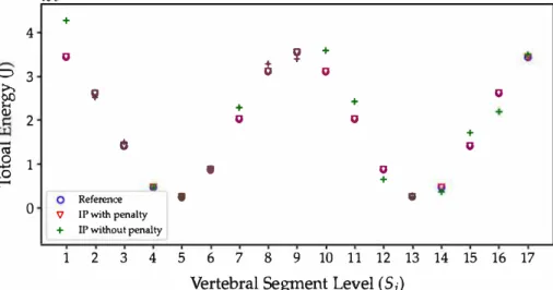
The direct problem was geometrically under-constrained and several admissible equilibria for 11eq have been obtained from energy minimization. Four solutions or deformation modes, Üe_{ql• lleq2, ueq3, lleq4, have been selected in Fig.} 2b. The convergence criterion of energy balance minimization was lower than 10-12• Calculations lasted between 0.2 s and 1 min CPU rime on a desk computer (Intel Xeon® 3.6GHz). The inverse problem algorithm was applied using u_eq1 as the targeted kinematic mode. It also played the role of uc previously introduced in paragraph 2.3.2. The initial vector of effective properties p, i.e., Ki, Bi and uf, was randomly generated with values between 0.5 X Pref and 1.5 X Pref·

Without using the penalty fonction c(p), the converged

solution _Psol slightly differed from the target _Pref as shown

in Fig. 3. However, the converged solution geometry Üe_q!

was perfect with aec !::! O. When c(p) was used with priors

corresponding with Pref• then both kinematic balance Üe_q!

Fig. 3 Test case with 34 wire­ frame elements: comparison of a resolution of the inverse problem (IP) with and without

penalty ₀

6'ô

1-< Q) "id

_....

₀ � 4 3 2 1 0 le-3 + 0 fil ô Referenœ V 1P with penalty + 1P without penalty

and effective properties Psol were predicted with aec !::! 0 and

the energy distribution fitted the reference energy (Fig. 3). A good convergence was obtained, as shown in Fig. 2c with computation rimes lower than 1 h CPU time.

3.2 Clinical application

For the clinical application, the fitting of spine balance Üeq on clinical data uc was excellent since aec was lower than 3 x 10-3 (Fig. 4a-c). As shown in Fig. 4d the convergence of the inverse problem was obtained for calculations lasting between 2 and 8 h (CPU rime) with a convergence criterion lower than 10-8• When the impact of distance fonction d and regularization fonction c (identical in 2014 and 2016) was exarnined, it was found that d(p501) was always lower than one third of c(p501). It showed that the penalty fonction was

properly chosen and did not altered the main purpose of the algorithm to fit clinical and modeled geometries.

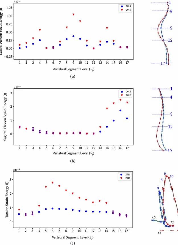
Table 1 summarizes the contribution of energy compo­ nents, i.e., compression, lateral bending, sagittal bending and torsion, to the total energy of the spine. Components were calculated into the segment local reference frame. In 2014, bending energy was predominant and that of lateral bending in the frontal plane greater than that in the sagit­ tal plane. The compression energy and torsion energy were found with a smaller percentage. The evolution in 2016 did not modify the prominence of bending but compressive energy decreased to the benefit of lateral and torsion energy. The distribution patterns of energies along the spine

are plotted in Fig. 5. Figure 5a shows an oscillation of

the lateral bending, especially marked in the apical zone (vertebral segment S8, S9, S10, corresponding to vertebrae T8-Tl l ) in 2014. For the evolving scoliosis in 2016, the energy peak strongly emerged and a noticeable increase was predicted in the lower junctional zone (S 14, cor­ responding to vertebrae L2-L3). The sagittal energy in

� +

li

0 0 + + 0 0 + 0

•

0 ₊

•

•

1 2 3 4 5 6 7 8 9 10 11 12 13 14 15 16 17

Fig. 4 Clinical application:

2 years follow-up of a

13-year-old girl (IA Lenke type, 40°

Cobb angle in 2014, 65° _Cobb angle in 2016). Spine balance obtained from clinical data and

inverse problem resolution: a

sagittal plane, b frontal plane, c

transverse plane. Convergence

of the inverse problem in d

with residual on the Jeft and

objective function/ values on the right 0 5 10 15 20 25 30 35 40 (a) Sagittal view

J

-5 0

...

_....

.

_{_.}

_...

_{. .}

5

-

Data 2014 - Data 2016 .. ,o ... Model 2014 .. ,v .. , Model 2016 Coronal view 0 -10 5 -8 10 _-6 15 -4 20 -2 25 0 30 35 2 40 4 -10 -5 0 5 (b) (c) L2

...,

•

Transverse view L5 L5 2,5 o.o -2.s -s.o

-:-

-...

..

10 20 30

..

....

• •

•

•

•

40 0 LO ·..;:; _<.> .2 0.8 :.:; _<.> <1.> o.e

.

..., 0.4

•

•

• •

-..._

0 10 20 30 40 Iteration Iteration (d)

Table 1 Clinical application: normalized percentage of total energy components in the wireframe mode) of the spine in 2014 and 2016 (13-year-old female patient, lA Lenke type)

EOS® _{exam date Compressive Flexion Laierai Torsion}

extension bencling

2014 18 52 19 10

2016 10 54 25 12

Fig. 5b showed an almost steady distribution up to the

junctional zone (S13, corresponding to L l-L2) followed

by a monotonie increase reaching its maximum value at the sacro-illiac junction (S 17, corresponding to L5-Sacrum). Scoliotic deformation exacerbated energy concentration in 2016. Concerning torsion energy Fig. 5c, the distribu­ tion was disrupted by a sudden increase before the apex (S5-S6, corresponding to T5-T7) and particularly marked in 2016. Maximum values were reached in the upper junc­ tional zone (S6, corresponding to T6-T7). It was also observed that the lower junctional zone (S 12, S 13, cor­ responding to Tl2-L2) showed a noticeable increase of torsion energy in 2016.

x.10-J ... -1 1.25

•

2014

s

y 2016 � 1.00 y

.,

C: _y � .5

..

0.75 y _y .t:I y (/) _0.50 C:

•

)( 0.25 y

•

• •

� y y y

•

y y

•

•

y

•

• •

...

0.00

• •

•

•

•

•

•

..

-0.25 2 3 4 5 6 7 8 9 10 11 12 13 14 15 16 17 ... ,-17- ....

Vertebral Segment Level (S;)

(a) xto-J 3

•

2014

s

y 2016 � y

.,

y C: � 2

-�

y

•

(/) § 1

•

•

·x

.,

•

•

f;:

•

:

y

]

_'6h 0

'

'

•

•

•

• •

•

•

•

(/) 1 2 3 4 5 6 7 8 9 10 11 12 13 14 15 16 17

Vertebral Segment Level (S;)

(b) x10-4

•

2014 3 y 2016 8

s

y � y y 9

.,

y &i 2 y

-�

y y _y .t:I y y y .§ 1 y

• • • • •

12

•

₁

:

•

• • • • •

'

'

'

LS 0 1 2 3 4 5 6 7 8 9 10 11 12 13 14 15 16 17 _LS Vertebral Segment Level (S;)

(c)

Fig. 5 Clinical application: 2 years follow-up of a 13-year-old girl (IA Lenlœ type, 40° _{Cobb angle in 2014, 65}° _{Cobb angle in 2016). Energy} distribution patterns: a lateral bending (frontal plane), b flexion-extension (sagittal plane), c torsion

4 Discussion

We initially hypothesized that a wireframe model based upon mechanical energy minimization might depict the spine balance in scoliosis time course. The governing equations and the associated numerical direct and inverse methods were first evaluated with a test case mimicking a simplified spine architecture, and second with a 2 years evolving scoliosis. The nonlinear response was searched in the form of successive piece-wise linear equilibria and in the vicinity of the equilibrium all forces derived from a local potential. Progressive results supported the proposed methodology and confirmed our central hypothesis.

We proposed the concept of mechanical effective tensor to condense, in a reduced number of scalars, the complex behavior of spine segments involving bones and soft tis-sues. Additionally, patient medical images constrained the inverse algorithm to check kinematic and mechanical bal-ances to warrant the clinical relevance of the methodol-ogy. The penalization process guided the inverse problem resolution among multiple numerical admissible solutions.

Despite the concept of effective tensors, the amount of unknowns was still diminished to diagonal components because they played major roles. While accelerating numeri-cal resolution, this choice provided convincing results com-pared to clinical diagnosis. However, the set of equations can predict the influence of coupled mechanical loading (i.e bending, torsion, compression) with enhanced clinical relevance by exploring the impact of extra diagonal terms

potentially asymmetric. Especially, this could improve predicting the structure nonlinear response due to loading history.

The time scale of the clinical follow-up, allowed us to assume that the AIS evolution could be considered as being a steady-state mechanical problem at each time observation. Two snapshots at 2 year intervals were selected to establish the clinical relevance of our pro-posed methodology. The domain was restrained to thoracic and lumbar segments. Indeed, cervical spine balance is rarely deformed by AIS and it is mainly determined by the dynamical maintain of horizontal sight.

AIS deformation was interpreted in terms of mechanical energies and this objective quantification allowed complet-ing the empirical clinical approach. As observed clinically, we found that the apical zone was playing a significant role in energy concentration, especially for lateral bending and

torsion. Beyond that, the prominence of sagittal bending found in sacro-illiac junction was also corroborated by pre-vious clinical studies (Brink et al. 2018). The junction zones located on both sides of the apex observed in clinics by curve inversion showed intrinsic variations of energies and notably for torsion. Indeed, these zones are examined to establish clinical diagnosis, AIS classification and surgical planning.

In this article, the energy distribution obtained from avail-able clinical data was calculated. This can be considered as the basis of further clinical studies on multicentric cohorts involving main types of AIS in Lenke classification and the concept of stable or unstable scoliosis. The implementation of specific algorithms will allow a prediction of scoliotic curve progression by the analysis of segments effective prop-erties. In that case, the clinically enriched models will be considered as being predictive models.

Acknowledgements The French Minister of Education and Research and The Children Hospital of Toulouse (France) are acknowledged for their assistance.

Compliance with ethical standards

Conflict of interest The authors declare that they have no conflict of interest.

Appendix 1: Rotation matrix

Rotation matrix Ri : (17) ⎛ ⎜ ⎜ ⎝

cos 𝜃icos 𝛼i − sin 𝜃icos 𝛼i sin 𝛼i

sin 𝜃icos 𝜑i+ cos 𝜃isin 𝛼isin 𝜑i cos 𝜃icos 𝜑i− sin 𝜃isin 𝛼isin 𝜑i − cos 𝛼isin 𝜑i

sin 𝜃isin 𝜑i− cos 𝜃isin 𝛼icos 𝜑i cos 𝜃isin 𝜑i+ sin 𝜃isin 𝛼icos 𝜑i cos 𝛼icos 𝜑i

⎞ ⎟ ⎟ ⎠

Appendix 2: Adjoint method

The derivative operator ∇𝐩 used on any function h(𝐮eq(𝐩), 𝐩)

is defined as:

Therefore,

Calling 𝐠(𝐮, 𝐩) = (∇𝐮V)(𝐮, 𝐩) , the definition of 𝐮eq for every

𝐩gives: (18) ∇_𝐩h= dh d𝐩 (19) ∇_𝐩f = 𝜕f 𝜕𝐮_eq d𝐮_eq d𝐩 + 𝜕f 𝜕𝐩. (20) 𝐠(𝐮_eq(𝐩), 𝐩) = 0 therefore ∇𝐩(𝐠(𝐮eq(𝐩), 𝐩)) = 0,

leading to the following equation:

Using this result in Eq. (19) gives:

The vector − 𝜕f 𝜕𝐮_eq ( 𝜕𝐠 𝜕𝐮_eq )−1

, often called 𝝀 , is the adjoint vec-tor. It is the solution of a linear system, faster to solve than an explicit finite difference calculation to access the gradient ∇𝐩f.

Appendix 3: Sensitivity study

In the proposed methodology, the spine balance was found by minimizing the total mechanical energy using EOS®

medical images from patient follow-up as input data. We assessed the impact of uncertainties of clinical data numeri-zation on numerical prediction.

The measurements errors were evaluated using ten numerizations of a single clinical image. The locations and orientations of seventeen vertebral bodies have been com-puted for each numerization. Inspired by Bayesian method-ology, the geometry space was described with a probability law chosen to be normal, i.e., defined by mean value and standard deviation. The first and last decile of the distri-bution provided the envelops of the clinical geometry. The maximum distance between the envelops was evaluated at 5% of the maximum displacement from vertical spine in both frontal and sagittal direction.

The computation cost for the uncertainties propagation through the inverse problem was prohibitive. Therefore, we investigated the propagation of hypothetical uncertainties on the parameters, through the direct problem. The parameters uncertainties were chosen to be independent and following a normal distribution with a fixed mean and an arbitrary initial standard deviation (few percents of the mean). The deciles distribution of the computed equilibrium geometry

𝐮_eq was then compared with the deciles of clinical data from

image numerization. The parameters standard deviation was iteratively updated to obtain a good match between clinical measurements envelops and equilibrium geometry envelops. After computation, the discrepancies between clinical envel-ops and equilibrium envelenvel-ops was lower than 6% and was obtained with uncertainties on parameters characterized by standard deviation of 5% of the mean values.

(21) d𝐮_eq d𝐩 = − ( 𝜕𝐠 𝜕𝐮_eq )−1 𝜕𝐠 𝜕𝐩. (22) ∇𝐩f = − 𝜕f 𝜕𝐮_eq ( 𝜕𝐠 𝜕𝐮_eq )−1 𝜕𝐠 𝜕𝐩 + 𝜕f 𝜕𝐩

References

Abelin-Genevois K, Estivalezes E, Briot J, Sévely A, de Gauzy JS, Swider P (2015) Spino-pelvic alignment influences disc hydra-tion properties after AIS surgery: a prospective MRI-based study. Eur Spine J 24(6):1183–1190. https ://doi.org/10.1007/s0058 6-015-3875-4

Albert T (2005) Inverse problem theory and methods for model parameter estimation. SIAM, Philadelphia 978-0-89871-792-1 Araújo Fábio A, Ana M, Nuno A, Howe Laura D, Raquel L (2017)

A shared biomechanical environment for bone and posture development in children. Spine J 17(10):1426–1434. https :// doi.org/10.1016/j.spine e.2017.04.024

Brink RC, Schlösser TPC, van Stralen M, Vincken KL, Kruyt MC, Hui SC, Viergever MA, Chu WC, Cheng JC, Castelein RM (2018) Anterior-posterior length discrepancy of the spi-nal column in adolescent idiopathic scoliosis-a 3d CT study. Spine J 18(12):2259–2265. https ://doi.org/10.1016/j.spine e.2018.05.005

Davidson JD, Jebaraj C, Narayan Y, Rajasekaran S, Kanna Rishi M (2012) Sensitivity studies of pediatric material properties on juvenile lumbar spine responses using finite element analysis. Med Biol Eng Comput 50(5):515–522. https ://doi.org/10.1007/ s1151 7-012-0896-6

Drevelle X, Lafon Y, Ebermeyer E, Courtois I, Dubousset J, Skalli W (2010) Analysis of idiopathic scoliosis progression by using numerical simulation. Spine 35(10):E407–E412. https ://doi. org/10.1097/BRS.0b013 e3181 cb46d 6

Ferguson Stephen J, Keita I, Lutz-P N (2004) Fluid flow and con-vective transport of solutes within the intervertebral disc. J Biomech 37(2):213–221. https ://doi.org/10.1016/S0021 -9290(03)00250 -1

Lafage V, Dubousset J, Lavaste F, Skalli W (2004) 3d finite element simulation of Cotrel–Dubousset correction. Comput Aided Surg 9(1–2):17–25. https ://doi.org/10.3109/10929 08040 00063 90

Lenke Lawrence G, Betz Randal R, Jürgen H, Bridwell Keith H, Cle-ments David H, Lowe Thomas G, Kathy B (2001) Adolescent idiopathic scoliosis : a new classification to determine extent of spinal arthrodesis. JBJS 83(8):1169

Ludescher B, Effelsberg J, Martirosian P, Steidle G, Markert B, Claus-sen C, Schick F (2008) T2- and diffusion-maps reveal diurnal changes of intervertebral disc composition: an in vivo MRI study at 1.5 Tesla. J Magn Reson Imaging 28(1):252–257. https ://doi. org/10.1002/jmri.21390

Meng X, Bruno AG, Cheng B, Wang W, Bouxsein ML, Anderson DE (2015) Incorporating six degree-of-freedom intervertebral joint stiffness in a lumbar spine musculoskeletal model-method and performance in flexed postures. J Biomech Eng 137(10):101008-1–101008-9. https ://doi.org/10.1115/1.40314 17

Newell N, Little JP, Christou A, Adams MA, Adam CJ, Masouros SD (2017) Biomechanics of the human intervertebral disc: a review of testing techniques and results. J Mech Behav Biomed Mater 69:420–434. https ://doi.org/10.1016/j.jmbbm .2017.01.037

Noailly J, Wilke H-J, Planell JA, Lacroix D (2007) How does the geom-etry affect the internal biomechanics of a lumbar spine bi-segment finite element model? Consequences on the validation process. J Biomech 40(11):2414–2425. https ://doi.org/10.1016/j.jbiom ech.2006.11.021

O’Connell Grace D, Wade J, Vresilovic Edward J, Elliott Dawn M (2007) Human internal disc strains in axial compression meas-ured noninvasively using magnetic resonance imaging. Spine 32(25):2860–2868. https ://doi.org/10.1097/BRS.0b013 e3181 5b75f b

Riseborough Edward J, Ruth W-D (1973) A genetic survey of idi-opathic scoliosis in Boston, Massachusetts. JBJS 55(5):974

Schultz AB, Warwick DN, Berkson MH, Nachemson AL (1979) Mechanical properties of human lumbar spine motion segments. J Biomech Eng 101:46–52

Stefan S, Burkhart Katelyn A, Allaire Brett T, Daniel G, Anderson Dennis E (2019) Musculoskeletal full-body models including a detailed thoracolumbar spine for children and adolescents aged 6–18 years. J Biomech. https ://doi.org/10.1016/j.jbiom ech.2019.07.049

Stokes Ian AF (2007) Analysis and simulation of progressive adoles-cent scoliosis by biomechanical growth modulation. Eur Spine J 16(10):1621–1628. https ://doi.org/10.1007/s0058 6-007-0442-7

Stokes Ian A, Mack G-M, David C, Laible Jeffrey P (2002) Meas-urement of a spinal motion segment stiffness matrix. J Biomech 35(4):517–521

Swider P, Pedrono A, Ambard D, Accadbled F, de Gauzy JS (2010) Substructuring and poroelastic modelling of the intervertebral disc. J Biomech 43(7):1287–1291. https ://doi.org/10.1016/j.jbiom ech.2010.01.006

Tingting Z, Tao A, Wei Z, Tao L, Xiaoming L (2015) Segmental quan-titative MR imaging analysis of diurnal variation of water content in the lumbar intervertebral discs. Korean J Radiol 16(1):139.

https ://doi.org/10.3348/kjr.2015.16.1.139

Tristan L, Claudio V, Raphael P, Jean D, Wafa S, Raphael V (2018) Shear-wave elastography can evaluate annulus fibrosus alteration in adolescent scoliosis. Eur Radiol 28(7):2830–2837. https ://doi. org/10.1007/s0033 0-018-5309-2

van der Plaats A, Veldhuizen AG, Verkerke GJ (2007) Numerical simulation of asymmetrically altered growth as initiation mecha-nism of scoliosis. Ann Biomed Eng 35(7):1206–1215. https ://doi. org/10.1007/s1043 9-007-9256-3

Villemure I, Aubin CE, Dansereau J, Labelle H (2004) Biomechani-cal simulations of the spine deformation process in adolescent idiopathic scoliosis from different pathogenesis hypotheses. Eur Spine J 13(1):83–90. https ://doi.org/10.1007/s0058 6-003-0565-4

Virtanen P, Gommers R, Oliphant TE, Haberland M, Reddy T, Cour-napeau D, Burovski E, Peterson P, Weckesser W, Bright J, van der Walt SJ, Brett M, Wilson J, Millman KJ, Mayorov N, Nelson Andrew RJ, Jones E, Kern R, Larson E, Carey CJ, Polat I, Feng Y, Moore EW, VanderPlas J, Laxalde D, Perktold J, Cimrman R, Henriksen I, Quintero EA, Harris CR, Archibald AM, Ribeiro AH, Pedregosa F, van Mulbregt P, Contributors SciPy 1 0 (2019) SciPy 1.0–fundamental algorithms for scientific computing in python. arXiv :1907.10121 [physics]

Violas P, Estivalezes E, Briot J, de Gauzy JS, Swider P (2007) Quantifi-cation of intervertebral disc volume properties below spine fusion, using magnetic resonance imaging, in adolescent idiopathic sco-liosis surgery. Spine 32(15):E405–E412. https ://doi.org/10.1097/ BRS.0b013 e3180 74d69 f

Publisher’s Note _{Springer Nature remains neutral with regard to}