A comparison of sediment transport models for combined current and wave flows

A Comparison of Sediment Transport Models for

Combined Current and Wave Flows

by

John Piero Gambino

Submitted to the Department of Civil and Environmental Engineering

in partial fulfillment of the requirements for the degree of

Master of Science in Civil and Environmental Engineering

at the

MASSACHUSETTS INSTITUTE OF TECHNOLOGY

February 1998

© Massachusetts Institute of Technology, 1998. All Rights Reserved.

A uthor

...

...

Department of Civil and Environmental Engineering

January

29,

1998

C ertified by ...

CrfdyOle

S. Madsen

Professor, Department of Civil and Environmental Engineering

Thesis Supervisor

A ccepted by ... ... ...

Joseph M. Sussman

Chairman, Departmental Committee on Graduate Studies

Department of Civil and Environmental Engineering

A Comparison of Sediment Transport Models for Combined

Current and Wave Flows

by

John Piero Gambino

Submitted to the Department of Civil and Environmental Engineering on January 29, 1998, in partial fulfillment of the

requirements for the degree of

Master of Science in Civil and Environmental Engineering

Abstract

Three models that predict sediment transport in combined wave-current flows were compared to determine which does the best job of modeling sediment transport in the coastal environment. The models compared were derived by Ackers and White (1973), Bailard (1981), and Madsen (1997). The Ackers and White model was derived for steady unidirectional flow and was modified by Scheffner (1996) to account for waves.

The assumptions made by the three models were analyzed and compared, and subsequently the predictions of the three models were also compared to determine the differences between the models. The analysis was first done for steady unidirectional flows to pinpoint differences in the models that were not specific to the combined wave-current flow. Major differences were found between the Madsen model and other two on how suspended load transport was calculated. These differences were magnified greatly when the predictions for combined wave-current flows were analyzed.

Analysis of the methods used by the different models indicate that the Madsen model does the best job of predicting sediment transport and that in the presence of large waves the other two models will over-predict the amount of sediment transport because of their deficiencies in accounting for the influence of waves in the calculation of suspended load transport.

Thesis Supervisor: Ole S. Madsen

Acknowledgments

I would like to begin by thanking my advisor, Ole Madsen, for the all guidance he has given me throughout my 6 years at MIT. I know that I would have had a much tougher time going through MIT had it not been for his influence. He is a great professor and friend.

I am also very grateful to all of the friends who have shared my MIT experiences and even though many have moved on to new lives, they will never be forgotten. I would especially like to thank Paulo Salles and Sanjay Pahuja (an expert in the properties of sand) for their eagerness to help me with any problem that I faced, especially the academic ones.

Most importantly, I would like to thank my family. I dedicate this thesis to my parents, for all their love and support and to my sister Maria. I would finally like to thank my cousin Nico for his advice about college, and his encouragement to become an engineer, despite the fact that he probably will not be able to understand much of this thesis.

Contents

1.0 Introduction

6

2.0 The Different Models for Pure Current

7

2.1 Ackers and White 7

2.2 Bailard 10

2.3 Madsen 15

2.3.a Bedload Transport 17

2.3.b Suspended Load Transport 19

3.0 Comparison of the Models for Pure Current

21

3.1 Description of the Differences 21

3.2 Discussion 22

4.0 How the Models Account for Waves

46

4.1 Ackers and White 46

4.2 Bailard 48

4.3 Madsen 53

4.3.a Bedload Transport 60

4.3.b Mean Suspended Load Transport 62

4.3.c Mean Wave-Associated Suspended Load Transport 64

5.0 Comparison of the Models for Combined Wave-Current Flows 65

5.1 Description of the Differences 65

6.0 Conclusion

104

1.0 Introduction

The modeling of sediment transport in the coastal environment is complex and quite diffi-cult. There are many factors that can influence sediment transport: waves, longshore currents, sed-iment size and density, storms and the slope of the bed. Predicting sedsed-iment transport is made even more difficult by the fact that these factors are highly variable, changing from one day to the next. Despite all of these difficulties, many models that try to predict sediment transport from these variables have been published. Knowing the sediment transport rate is quite useful because it helps to predict how often a harbor needs to be dredged, or how long a cap over a dumped con-taminant can last before it is eroded away. It is also important in determining how beaches change due to waves, which is especially important to people who live close to or on a beach.

This paper examines three models of sediment transport, comparing how they account for each of the different variables that influence sediment transport and by analyzing the predictions made by these models when these variables change. The models examined are from Ackers and White (1973), Bailard (1981) and Madsen (1997). Linear waves are assumed for the analysis, without breaking, which makes the analysis valid for areas outside of the surf zone. Since the pre-diction of sediment transport is at best an estimate, compounded by the fact that we are trying to model the real coastal environment which is constantly changing, the exact answers are not known, so the patterns and trends of the predictions are looked at instead, to explain how and why each model predicts what is does.

This paper begins by reviewing each model, first for unidirectional flows and then for combined wave-current flows, summarizing the method of calculation used and the assumptions made by each model. The analysis begins by comparing the predictions made by the models for steady unidirectional flows, and then they are compared for combined wave-current flows. This is

done to examine why the models predict different results; to see whether they differ in their basic predictions of sediment transport in steady unidirectional flows or whether the differences are due

to how they account for waves.

2.0 The Different Models for Pure Current

2.1 Ackers and White

The Ackers and White model for sediment transport is developed from a theory given by Ackers (1972). Ackers and White (1973) are seeking to develop a new framework for the analysis of transport data. In order to calculate the stream's transporting power, they are using the average stream velocity instead of the shear velocity. Dimensional analysis is used and the theory avoids refinements that the authors believe do not add much to the accuracy of the model.

Ackers and White (1973) state that there are seven variables needed to calculate the sedi-ment transport of a unidirectional flow: sedisedi-ment diameter; specific gravity of the sedisedi-ment; mean velocity of the flow; shear velocity (which can be determined from the velocity distribution of the flow or the depth/slope relationship); depth of flow; kinematic viscosity of the fluid; and the accel-eration due to gravity. The sediment transport rate (Qs) in a steady unidirectional flow is given by

Qs

= _{i C r 1.0 u (1)}

U = depth-averaged current velocity

U* = shear velocity

Fgr = sediment mobility number

A, C, m, and n are dimensionless variables calculated from equations 3 through 10.

The result,

Qs,

is in units of volume per length per time. In order to use this equation, the dimen-sionless grain diameter, which is the cube root of the ratio of immersed weight to viscous forces, applicable to both coarse, transitional and fine sediments, needs to be calculated. Coarse sediment is sediment that is transported mainly as bedload while fine sediment is transported mainly as sus-pended load. The dimensionless grain diameter is given by

Dgr= dg( )]1/3 (2)

Where g = acceleration due to gravity s = specific gravity of the sediment 1 = the kinematic viscosity of the fluid

Once the dimensionless grain diameter is calculated, the following variables can be determined: If Dgr > 60.0,

I =0 (3)

m = 1.5 (4)

A = 0.17 (5)

If 1.0 < Dr < 60.0,

n = 1.00 -0.56 log (Dgr) (7)

m =(9.66 / Dgr) + 1.34 (8)

A = (0.23/ r ) + 0.14 (9)

log C = 2.86 log (Dg_r) - (log Dgr)2 - 3.53 (10)

The shear velocity can be found if the Chezy coefficient is calculated. The formula given below for the Chezy coefficient (C-) is valid only for metric units. C, and the number 18 are in units of meters1/2 / second. Once the Chezy coefficient is calculated, the shear velocity, U,, can be calculated (Scheffner 1996).

C = 18 log12d ₍₁₁₎

U, = U (12)

C_

h = flow depth

U = average flow velocity

Dimensionless expressions for sediment transport were derived using the stream power concept, which bases transport on the available power of the flow. There are different transport modes, depending on whether the sediment is coarse or fine. For fine sediment, the total stream power is

used to determine the power per unit area available while for coarse sediment, the power per unit area of the bed is the product of net grain shear and shear velocity. This leads to the development of a term for the efficiency of the transport. Ackers and White hypothesize that efficiency is dependent on the sediment mobility number, which is "the ratio of the shear force on unit area of the bed to the immersed weight of a layer of grains" (1973). The sediment mobility number is given by

Fa (13)

Fgr = gd(s - 1) 13o2 h

Theta (0) was determined experimentally from flume data and

e

should be set equal to 10. Once the sediment mobility number is calculated, all the variables needed for equation 1 are known and the sediment transport can be calculated. Equation 1 can be used for a range of sediment diame-ters from 0.04 mm to 4 mm (0.00004 m to 0.004 m).

2.2

Bailard

The basis for the Bailard model of sediment transport comes from the energetics-based total load sediment transport model for streams developed by Bagnold (1966). The Bagnold method is an attempt from the general to the particular and the uncertainties about turbulence effects, such as those of boundary roughness, form drag. and sediment transport, on the flow resis-tance have been avoided by treating the mean flow velocity and the tractive force as independent, or given, variables. Bagnold justifies this by stating that "the objective is to predict the transport of

solids by the fluid flow and not to attempt to predict fluid flow itself, which lies within the proper province of the hydraulic engineer" (Bagnold 1966).

Bagnold's model is applicable to streams and rivers with the following four restrictions: steady open-channel flow by gravity; unlimited availability of transportable solids; the concentra-tion of transported solids, by immersed weight, is sufficiently small that the contribuconcentra-tion of the tangential gravity pull on the solids to the applied tractive stress can be neglected; and the system considered is defined as statistically steady and as representative not of conditions at a single cros-section but average conditions along a length of channel sufficient to include all repetitive irregu-larities of slope, crossection, and boundary.

Bagnold states that there are two ways by which sediment can be transported: through bedload and through suspended load. Bedload is supported by the bed via grain to grain interac-tions, while suspended load is supported by the fluid via turbulent diffusion. In either case, energy is used by the stream to transport the sediment. For steady flow, Bailard (1981) used Bagnold's theory to develop the following total load sediment transport equation:

i = + +(W/U) tanfn (14)

s tano-tanp (W/U)-Est

where i is the immersed weight per unit width per unit time, the subscript B refers to bedload and the subscript S refers to suspended load. 3 is the slope of the stream bed,

4 is the internal angle of

friction for the sediment, W is the fall velocity of the sediment (given by equation 45), E is the load efficiency, U is the mean velocity of the stream, and 2 is the rate of energy dissipation of the stream, given by

0 = ru = pCU (15)

where T is the shear stress at the bed, p is the density of water and Cf is a friction coefficient, taken equal to 0.003 from experimental data. Bagnold (1966) found the load efficiencies experimentally, and for stream flow found EB roughly equal to 0.13, Fs roughly equal to 0.01, and tan 4) can be taken as roughly equal to 400. The immersed weight per unit width per unit time (i) can be related to the sediment transport, Qs, by

i = (s- 1)pgQs (16)

where s is the specific gravity of the sediment. Bailard's (1981) derivation of equation 14 leads to a different result for the suspended load transport than the one Bagnold developed. Bailard begins with the analysis of a simple two dimensional flow over a plane bed with slope tan 3. The depth of the flow is h, and the velocity is a function of z, expressed as u(z). The z coordinate is perpendic-ular to the bed while the x coordinate is directed down'slope (parallel to the flow). The rate of

energy dissipation of the stream, Ostream, is given by

Qstream = Jpagsinpi3 * idz (17)

Pa = (p -p)N + p (18)

where Pa is the apparent density of the water (accounting for the inclusion of sediment in the water), N is the local volume concentration of solids, and p is the density of pure water. Combin-ing equations 17 and 18 yields:

stream - (P -p)gsinl3 NN idz + (19)

Q is the sediment-free stream power, given by equation 15. According to Bagnold (1966), the

immersed weight suspended sediment transport rate per unit area bed, is is defined by

s = (ps-p)gcoSfp oNUdz (20)

According to Bagnold (1966), the rate of energy dissipation per unit area of bed associated with this transport of sediment, Qsed, is equal to the sediment load times its fall velocity:

Qsed = (ps-p)gcospW3jNdz (21)

Where W is the sediment fall velocity. Combining equations 20 and 21 yields:

-sed - (22)

Nd d

j

Ndz

A critical aspect of Bagnold's model is his hypothesis that the rate of energy dissipation associated with the suspended sediment transport is related to the total rate of energy production of the stream through a constant of suspended load efficiency, es (Bailard, 1981). This can be expressed with the following equation:

By combining equations 19, 20, 22, and 23, and assuming u = U (the depth-averaged velocity), Bailard obtains the equation for the magnitude of the suspended sediment transport rate:

Is = ESl (tanis i + Q) (25)

It is important to note that this result is not identical the one derived by Bagnold. Rearranging equation 25 yields a result that can be compared to Bagnold's:

I

s

=

(26)

[(W/U) -Fstan ](26)

While Bagnold's paper yields the following equation:

s =(lEB) (27)

[(W/U) - tan] (27)

Bagnold derived this result while assuming that the stream power contribution from the sus-pended sediment load contributes directly to the sussus-pended sediment transport rate instead of through an efficiency factor (which is what Bailard assumes). There is hardly a difference between equations 26 and 27 for small bedslopes, which is fine for river flow, but this is not the case for equilibrium beach profiles. If U exceeds W/tan

3,

equation 27 predicts negative or infinite transport, which is obviously incorrect. Equations 15 and 26 correct for this by including Es in the denominator. Since 1/_s is roughly equal to 41, it is quite difficult for equation 26 to yield negative or infinite transport. Since the ultimate purpose of this paper is to compare flows including both waves and current in the coastal environment, the Bailard result will be used.

There is one other difference between Bagnold's and Bailard's derivations. Bagnold multi-plies the suspended load transport by 1-EB, because the energy that has been dissipated in bedload

transport cannot go into suspended load. Bailard simply incorporates this into his ES, so there is a slight difference between Bagnold's Es and Bailard's ES. Bagnold states that equation 27 is equal to 0 for laminar flow.

2.3 Madsen

The Madsen model (1997) takes into account the formation of dunes and other effects that the flow may have on the bed surface, but since the other models do not take this into account, I am going to neglect this aspect (only for pure current, however) of the Madsen model in order to make a more logical comparison of the models. This will enable me to eliminate this added fea-ture of this model as a potential source of differences with the other models.

The following variables are needed to begin the calculation of sediment transport in a steady unidirectional flow (such as a river):

Uc = the current velocity at a specified height (zr) above the bottom z, = the height were the current velocity is specified

h = water depth

d = _{median sediment diameter (d50)}

ps = sediment density (assumed = 2, 650 kg/m3 for quartz)

p, = p = water density (assumed = 1, 025 kg/m3 for seawater)

[ = slope of bottom measured from horizontal (positive if flow is downhill) u = kinematic viscosity of fluid (molecular = 10-6 m2/sec for seawater)

If Uc. at Zr, is not given, it can be calculated if the depth-averaged current velocity is known. I used metric units for all of my calculations. All lengths are in meters, times in seconds, veloci-ties in meters per second, stresses in pascals, etc.

Many of the variables in the equations contain subscripts. The meaning of these sub-scripts are listed below:

()b = conditions at the bottom

()c = quantity associated with current

()cr = quantity associated with critical conditions for initiation of sediment motion

Since we are dealing with flows over a plane bed, the Nikuradse equivalent bottom rough-ness, k,,, is equal to the sediment diameter, d. The first thing we need to know is whether the flow is rough turbulent or smooth turbulent:

If k,,U*,/v > 3.3, the flow is rough turbulent and

(28)

1o- ₃₀

If k,,U*c/v < 3.3, the flow is smooth turbulent and

zo = v/9U*c

This leads to the calculation of the shear velocity (U*c) and current friction factor (f,):

U,*_c = U c9

(29)

fc = _{1 (31)} 4log(j

Unfortunately, U*c has different solutions according to whether the flow is rough turbulent or not because this affects the computation of zo. Another problem is the fact that it is not known whether the flow is rough turbulent or smooth turbulent unless U*c is known, which is one of the variables that we are solving for. To solve these equations, it is assumed that the flow is rough tur-bulent, and then the condition is checked after the calculation. If the flow is indeed rough turbu-lent, the solution remains the same. If, however, the flow proves to be smooth turbuturbu-lent, equations 29 through 31 need to be solved iteratively.

Knowing U*c enables the total shear stress to be calculated:

T = pU;c (32)

2.3. a Bedload Transport

The Shields Parameter can be calculated from:

V= ₍₃₃₎

(s- l)pgd

where s = ps/p,. For transport to occur, the Shields parameter calculated in equation 33 must be greater than a critical Shields parameter. The following equations calculate the critical Shields parameter:

d S. = - ,((s- 1)gd) 4v (34) If S, < 0.8 -2/7 1cr = 0.1S S If S* > 300 (36) If 0.8 < S, < 300 (35) 0.24 cr 2/3 2/3 4 s* 423$ 2/3 +0.055 (3-7e-4 50

This value for the critical Shields parameter does not take slope into effect. The complete

parame-ter, WVcr.p, is presented by

cr.p = COS P(l tanops cr (38)

Where s, = 50'. A generalized form of the Meyer-Peter and Muller bedload transport formula

allows the bedload to be calculated:

F(3) = cos" 1 -tan-- (39)

tan

4,)

Where 0,,, = 30'

B = qSB 8 3/2

s(9-F( )) (40)

d

(s- 1)gd F(P)(F( )

Where qSB is the bedload. Note that for transport to begin, the Shields parameter must be greater than the critical Shields parameter (accounting for slope). If X is less than vcr, p, there will be no transport. The reason why the bedload formula has a different internal angle of friction (,, versus Os) is because the angle of kinetic (moving) friction must be overcome during transport while for the initiation of motion, the angle of static friction must be surpassed.

2.3.b Suspended Load Transport

The calculation of the suspended load transport begins with the calculation of the sediment reference concentration:

qSB

Ca = (0.4 Cb) s (41)

Where Cb is the concentration in the bottom (E is the sediment porosity. assumed = 0.35).

Cb = 1 - E = 0.65 (42)

a = 7d (43)

U, = 11.6U* (44)

W = J(s- 1)gd

5.1

+ 0.9

The next step is to calculate the suspended sediment concentration:

C(z) = Ca

KU cc

This leads to the equation for suspended load transport:

qss = 0.4Cb[I (a*,Z)lnh/z - ₂(a*, Z)]

Where h -- 1 I1 = 0.2 16 (a 1-Z Ina* I1 1I = 0.216 + 1-Z 1-Z (45) (46) (47) (48) (49) (50) (51)

3.0 Comparison of the Models for Pure Current

3.1 Description of the Differences

The Ackers and White model (1973) is the simplest of the three. It does not specifically calculate a bedload and suspended load, like the Madsen (1997) and Bailard (1981) models. This model is limited by the fact that it does not take bed slope into effect, which may not be important for river beds, where the slope is usually small, but this cannot be assumed correct for the coastal environment, where equilibrium bed slopes are generally steeper than river beds. The Ackers and White model was derived using an energetics approach.

The Bailard model, like Ackers and White's, is derived using an energetics approach. Unlike the other two models, however, it does not take water depth into account when calculating transport. Another difference between this model and the others is the fact that it does not incor-porate a critical shear stress for the initiation of motion. Both the Madsen model and the Ackers and White model give no transport until a critical shear stress is reached, which makes physical sense. The Bailard model will always give a transport, no matter how small the shear stress. The Bailard model also relies on experimental data for the calculation of the parameters es, eB, and Cf, which are needed to calculate the transport.

The Madsen model is unique in its accounting for changes in the bed surface due to the flow (though this is neglected for the pure current comparison). Unlike a laboratory, where the bed may contain immovable roughness elements, real beds change because of the flow, and this changes the flow's boundary layer and total transport. The Madsen model was derived using a mechanics approach. Like the Bailard model, the Madsen model gives two components of the

transport: a bedload and a suspended load, and takes bedslope into effect. The Madsen model, like the Ackers and White model, takes water depth into account and incorporates a critical Shields parameter that must be overcome in order for any transport to occur.

3.2 Discussion

In order to compare the models numerically, I programmed the three models and ran them with the same set of conditions.The Madsen model was modified to neglect changes in the bed due to the flow. Since the Ackers and White model does not account for bed slope, it was taken as zero for all of the runs. The water depth was set at 5 meters, but runs were also performed at a water depth of 2.5 meters to check if the Bailard model could neglect water depth without a large error. Transport was compared for three different grain diameters: 0.1 mm, 0.2 mm and 0.5 mm. Tables 1 and 2, given on pages 23 and 24, contain the output of these runs for all three models. For each of these conditions, transport was plotted versus current velocity. These figures are presented after the tables. As expected, transport increased with increasing current velocity for every single grain diameter and model. This occurred because with everything else held constant, increasing the flow velocity increases the shear on the bed and therefore the transport.

The first analysis I performed was to determine the effect of water depth on the transport for the Ackers and White model and the Madsen model. Figures 1 through 3 (pages 25 through 27) reveal that for all three grain sizes, transport increases as the water depth decreases for the Ackers and White model, while Figures 4 through 6 (pages 28 through 30) show the results for the Madsen model: the change in transport depends on the sediment size.

coefficient is used to calculate the shear velocity and is in the denominator of equation 12, this serves to increase the shear velocity in the Ackers and White model. An increased shear velocity leads to a greater sediment transport.

Table 1

Total Transport Versus Grain Size and Depth Averaged Current Velocity, depth = 5 m.

Madsen Total Load (mn3/m*sec) 0 1.70779E-08 3.40001 E-06 2.02127E-05 0.000136492 0.000226982 0.000548536 0.001152578 0.003947541 0.010471126 0 1.26925E-09 5.88167E-07 1.95439E-06 6.03565E-06 8.14627E-06 1.40142E-05 2.30587E-05 5.95482E-05 0.000151946 0 6.37291 E-09 1.51138E-06 5.177E-06 1.14343E-05 1.73364E-05 3.41879E-05 5.92814E-05 9.47408E-05 0.000143175

Ackers & White Total Load (mr3/m*sec) 0 4.50052E-15 8.44351 E-09 2.03591 E-07 3.53246E-06 7.1938E-06 2.41488E-05 6.62074E-05 0.000335313 0.001207404 0 0 3.18143E-08 5.61782E-07 5.17487E-06 8.77888E-06 2.12839E-05 4.40313E-05 0.00013974 0.000344773 0 0 5.72398E-07 6.41933E-06 2.20867E-05 4.01104E-05 0.000100227 0.000201364 0.000354473 0.000570743 Bailard Total Load (m3/m*sec) 1.22554E-05 1.36008E-05 3.98589E-05 8.16573E-05 0.000196932 0.00025415 0.000405002 0.00061473 0.001266752 0.00233629 4.32738E-06 4.76527E-06 1.20626E-05 2.40188E-05 5.62127E-05 7.1984E-05 0.000113207 0.000169989 0.000344537 0.000627773 3.83587E-06 4.149E-06 1.1456E-05 2.55418E-05 4.96083E-05 7.30541 E-05 0.000143532 0.000255387 0.000422213 0.000659528 Case # 1 2 3 4 5 6 7 8 9 10 11 12 13 14 15 16 17 18 19 20 21 22 23 24 25 26 27 28 29 30 Vc (m/sec) 0.37 0.38 0.5 0.6 0.75 0.8 0.9 1 1.2 1.4 0.38 0.39 0.5 0.6 0.75 0.8 0.9 1 1.2 1.4 0.44 0.45 0.6 0.75 0.9 1 1.2 1.4 1.6 1.8 d (mm) 0.1 0.1 0.1 0.1 0.1 0.1 0.1 0.1 0.1 0.1 0.2 0.2 0.2 0.2 0.2 0.2 0.2 0.2 0.2 0.2 0.5 0.5 0.5 0.5 0.5 0.5 0.5 0.5 0.5 0.5

--Table 2

Total Transport Versus Grain Size and Flow Velocity, depth = 2.5 m.

Madsen Ackers & White Bailard Total Load Total Load Total Load Case # Vc (m/sec) d (mm) (mA3/m*sec) (mA3/m*sec) (mA3/m*sec)

1 2 3 4 5 6 7 8 9 10 0.37 0.38 0.5 0.6 0.75 0.8 0.9 1 1.2 1.4 0.38 0.39 0.5 0.6 0.75 0.8 0.9 1 1.2 1.4 21 0.44 22 0.45 23 0.6 24 0.75 25 0.9 26 1 27 1.2 28 1.4 29 1.6 30 1.8 0.1 0.1 0.1 0.1 0.1 0.1 0.1 0.1 0.1 0.1 0.2 0.2 0.2 0.2 0.2 0.2 0.2 0.2 0.2 0.2 0.5 0.5 0.5 0.5 0.5 0.5 0.5 0.5 0.5 0.5 7.5933E-08 1.56398E-07 5.39471 E-06 2.72187E-05 0.000156057 0.000248718 0.000559253 0.001108142 0.00353607 0.008762145 2.35026E-08 5.36783E-08 8.93687E-07 2.66239E-06 7.86407E-06 1.05808E-05 1.82536E-05 3.03538E-05 8.03477E-05 0.00020532 6.85692E-08 1.2427E-07 2.22614E-06 6.85658E-06 1.46224E-05 2.19084E-05 4.2671 4E-05 7.36238E-05 0.000117539 0.000177922 2.73297E-1 3 2.8401 E-12 2.23099E-08 3.9517E-07 5.81739E-06 1.14996E-05 3.69809E-05 9.84441 E-05 0.000480064 0.001688886 0 0 8.6669E-08 9.77082E-07 7.53848E-06 1.2426E-05 2.89474E-05 5.83258E-05 0.000179146 0.000433457 0 0 1.25176E-06 9.30826E-06 2.89802E-05 5.09146E-05 0.000122512 0.00024104 0.000418712 0.000668004 1.22554E-05 1.36008E-05 3.98589E-05 8.16573E-05 0.000196932 0.00025415 0.000405002 0.00061473 0.001266752 0.00233629 4.32738E-06 4.76527E-06 1.20626E-05 2.40188E-05 5.62127E-05 7.1984E-05 0.000113207 0.000169989 0.000344537 0.000627773 3.83587E-06 4.149E-06 1.1456E-05 2.55418E-05 4.96083E-05 7.30541 E-05 0.000143532 0.000255387 0.000422213 0.000659528

S14

-12

40

-0.2 0.4 0.6 0.8 1 1.2 1.4

Depth-Averaged Current Velocity (imsec)

Figure 1. The Ackers and White model, total sediment transport rate versus depth-averaged cur-rent velocity for 0. 1 mm diameter grains.

0.5 0.6 0.7 0.8 0.9 1 1.1 1.2 1.3 1.4

Depth-Averaged Current Velocity (m/sec)

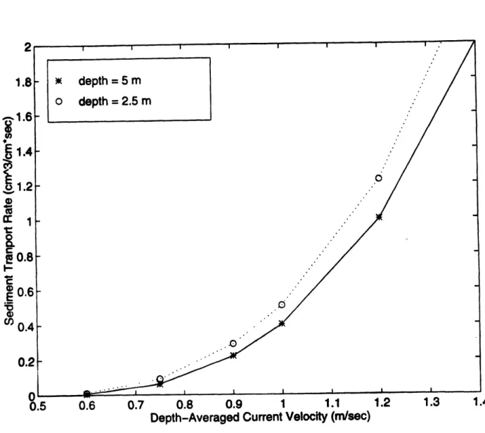
Figure 2. The Ackers and White model, total sediment transport rate versus depth-averaged cur-rent velocity for 0.2 mm diameter grains.

1.8 -. 1.6

1

I 1.4 ~ 0. 0.8 C 0.4 0.2 0_{0.5 066 0.7 0.8 0.9 1} 1.1 1.2

Depth-Averaged Current Velocity (m/sec)

Figure 3. The Ackers and White model, total sediment transport rate versus depth-averaged cur-rent velocity for 0.5 mm diameter grains.

120

K depth= 5 m 100 o depth = 2.5 m 80-0 a: 60-o 40 ._ I-20 0 0.2 0.4 0.6 0.8 1 1.2 1.4

Depth-Averaged Current Velocity (m/sec)

Figure 4. The Madsen model, total sediment transport rate versus depth-averaged current velocity for 0.1 mm diameter grains.

2.5 1 I X depth = 5 m o depth = 2.5 m -O CE 2-1.5 0. 0.0 O " 0.5 0'. 0.2 0.4 0.6 0.8 1 1.2 1.4

Depth-Averaged Current Velocity (m/sec)

Figure 5. The Madsen model, total sediment transport rate versus depth averaged-current velocity for 0.2 mm diameter grains.

(00.6

_.

E 0.5 -00 CC 0.4 .0.3 E O

S0.2

.. 0 0.1 .5 0.6 0.7 0.8 0.9 1 1.1 1.2 1.3 1.4

Depth-Averaged Current Velocity (m/sec)

Figure 6. The Madsen model, total sediment transport rate versus depth averaged-current velocity for 0.5 mm diameter grains.

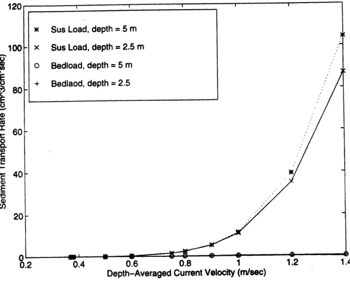
The effect of water depth is more complex in the Madsen model. The decreased water depth decreases the height above the bed where the given velocity is occurring, increasing the shear stress and the bedload. This is the same result as the Ackers and White model, but the sus-pended load reacts differently to the decreased depth. The decreased water depth lowers the total amount of sediment that can be held in suspension. With less sediment in suspension, there is less transport. This is especially true for small sediment, because suspended load comprises more of the total transport for fine grains than it does for large grains. Suspended load also depends on the shear stress, and an increased shear stress results in an increased suspended load. In the Madsen model, suspended load also increases with decreased depth, except for the 0.1 mm grains (figure 4). Figures 7 through 9 (pages 32 through 34) break down the Madsen transport into suspended load and bedload. Figure 7 reveals that at high enough current velocities, suspended load actually decreases with the smaller depth, despite the fact that the bedload increases, because the 0.1 mm sediment is small enough to have a large suspended load. Such a large suspended load will be more affected by a decrease in the water depth.

At very low flow velocities (less than 0.3 m/sec) only the Bailard model yields a transport because the flow is not strong enough to initiate movement according to the other two models. Table 1 (page 23) contains the output for the three models (at 5 meter depth). Table 1 reveals that the Madsen model predicts initiation of motion at lower flow rates than the Ackers and White model for the 0.2 mm and 0.5 mm grain sizes.

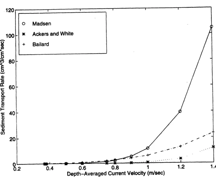
Figures 10 through 12 (pages 35 through 37) plot the sediment transport for each sediment size. for a flow depth of 5 meters. The plots show that the Madsen model is the most sensitive to grain size. When the sediment is small, the Madsen model predicts the largest transport of the three models, while the opposite is true for the larger grains: the Madsen model predicts the

low-est transport. 120 100 80 F 60 40 -20 -n 0.4 0.6 0.8 1 1.2 1.4

Depth-Averaged Current Velocity (n/sec)

Figure 7. The Madsen model, break down of the total sediment transport rate versus depth-aver-aged current velocity for 0. 1 mm diameter sediment.

K Sus Load, depth = 5 m x Sus Load, depth = 2.5 m o Bedload, depth = 5 m + Bedlaod, depth = 2.5 -J 'K *. .1 -°" I a _ W % - - le I ,

I

0.2 0.2

0.4 0.6 0.8 1 Depth-Averaged Current Velocity (m/sec)

p

1.2 1.4

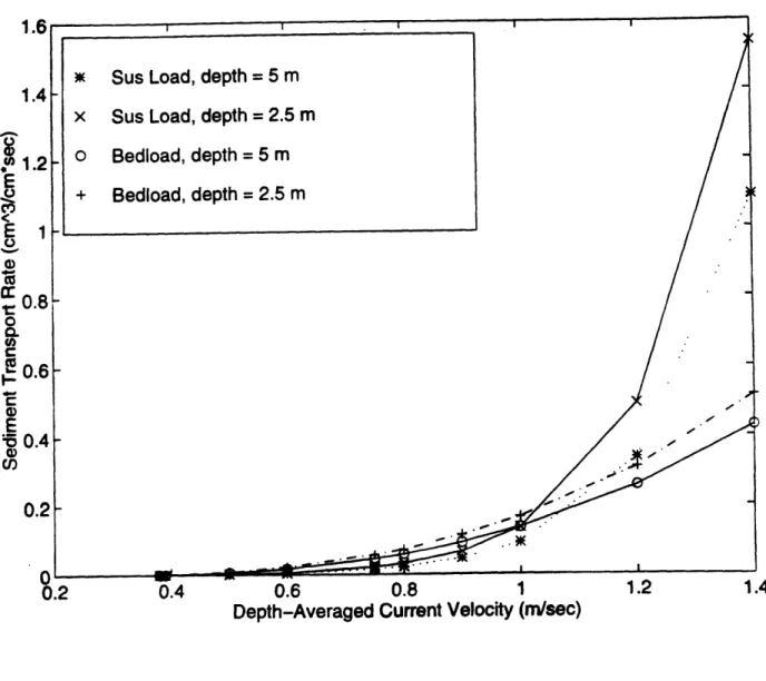
Figure 8. The Madsen model, break down of the total sediment transport rate versus depth-aver-aged current velocity for 0.2 mm diameter sediment.

m Sus Load, depth = 5 m

x Sus Load, depth = 2.5 m o Bedload, depth = 5 m + Bedload, depth = 2.5 m 1.6 1.4 .2 -0.8 0.6 0.4 0.2 I I I u 4 d d ~L ' Sc~ L 0.2 A I

0.8

* Sus Load, depth = 5 m 0.7

x Sus Load, depth = 2.5 m

S0.6 o Bedload, depth = 5 m + Bedload, depth = 2.5 m 0.5 0.4 o S0.3 -E -5 0.2 -" 0.1

-.4 0.5 0.6 0.7 0.8 0.9 1 1.1 1.2 1.3 1.4

Depth-Averaged Current Velocity (m/sec)

Figure 9. The Madsen model, break down of the total sediment transport rate versus depth-aver-aged current velocity for 0.5 mm diameter sediment.

120

o Madsen

100 w Ackers and White

+ Bailard 6 80 a 60 S40-E 20 0- 4-0.2 0.4 0.6 0.8 1 1.2 1.4

Depth-Averaged Current Velocity (m/sec)

Figure 10. The total sediment transport rate versus depth-averaged current velocity for 0.1 mm diameter sediment and a flow depth of 5 m.

+ Bailard CL 03 C 0 / 40.2 .4 .6 0.8 1 1.2 1.4

:Depth-Averaged Current Velocity (m/sec)

Figure 11. The total sediment transport rate versus depth-averaged current velocity for 0.2 mm

.-4

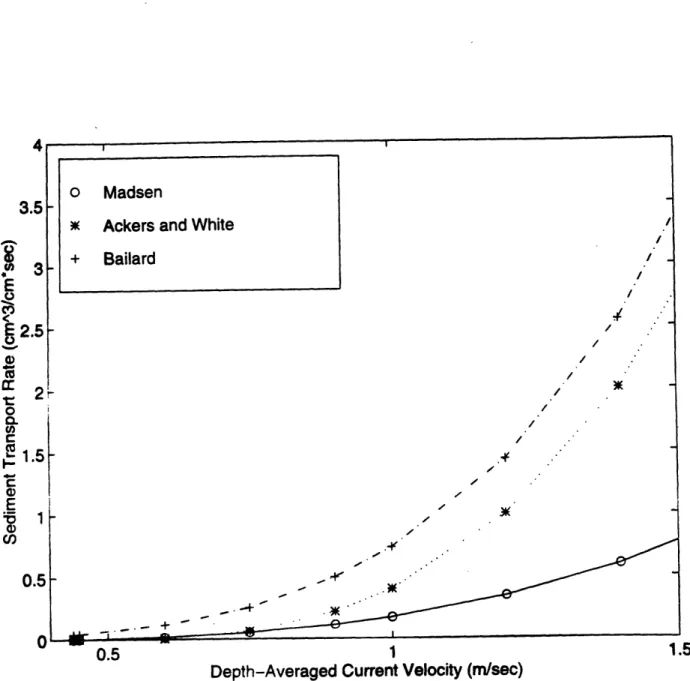
o Madsen

3.5-K Ackers and White

3- + Bailard E I E2.5 -0 / / . E C 0.5 01 0.5 1 1.5

Depth-Averaged Current Velocity (m/sec)

Figure 12. The total sediment transport rate versus depth-averaged current velocity for 0.5 mm diameter sediment and a flow depth of 5 m.

Figures 13 through 15 (pages 39 through 41) break down the total transport of the Bailard and Madsen models into suspended load and bed load. These figures show that the main differ-ence between these two models is in the suspended load. Suspended load is very dependent on grain size in the Madsen model, and this leads to the high fluctuations in the transport (mainly because of the change in suspended load) based on grain size. The Bailard suspended load is more constant: it is less dependent on grain size than the Madsen model. For all three grain sizes, sus-pended load is greater than the bedload based on the Bailard model (except at very low flow rates). This is not the case for the Madsen model, where Bedload dominates for the larger grains because large grains are less likely to be held in suspension by the water column.

Each model predicts a large increase in transport for increasing flow velocities. The Mad-sen model predicts the largest increase with flow velocity for the smallest sediment examined, mainly because of the increased suspended load, while the Ackers and White model predicts the largest increase for the larger sediments. While the Madsen model is the most sensitive to grain size, the Ackers and White model is the most sensitive to current velocity.

The Bailard model appears to be the least sensitive to changes in current velocity and grain size. It usually predicts the largest transport rates, regardless of the conditions. The other models, however, vary greatly according to the given conditions, with the Madsen model predicting very high transport only for fine sediment, and the Ackers and White model predicting a large transport for high flow conditions and large sediment. Examination of Tables 1 and 2 reveal that the Bailard model is within the range of the other two models for the two depths, indicating that for average flow depths, the Bailard model's omission of water depth may not be that significant. It should be stressed, however, that the Bailard model would overestimate the suspended load for fine sedi-ments if the flow depth was very low because it would assume that the suspended sediment would

extend up the water column until the suspended sediment concentration reached zero, which would happen at a significant height above the bottom. This, however, cannot happen because of the low flow depth.

12

10

4

0

* Sus Load, Madsen

0 - x Sus Load, Bailard o Bedload, Madsen

+ Bedload, Bailard

0

-

0-0.2 0.4 0.6 0.8 1

Depth-Averaged Current Velocity (m/sec)

1.2 1.4

Figure 13. Break down of the total sediment transport rate versus depth-averaged current velocity for the Madsen and Bailard models. Taken for 0.1 mm diameter sediment and 5 m flow depth.

8

W Sus Load, Madsen

5 x Sus Load, Bailard o Bedload, Madsen E O + Bedload, Bailard 3-0 0.0.4 0. 0.8 1 1.2 1.4 CD•_{0.2 0.4 0.6 0.8} 1 1.2 1.4 Depth-Averaged Current Velocity (m/sec)

Figure 14. Break down of the total sediment transport rate versus depth-averaged current velocity for the Madsen and Bailard models. Taken for 0.2 mm diameter sediment and 5 m flow depth.

$-r

... ... . . .

1.5

0.5 1

Depth-Averaged Current Velocity (m/sec)

Figure 15. Break down of the total sediment transport rate versus depth-averaged current velocity for the Madsen and Bailard models. Taken for 0.5 mm diameter sediment and 5 m flow depth.

* Sus Load, Madsen

x Sus Load, Bailard o Bedload, Madsen + Bedlaod, Bailard 2.5 - 2-O It E 0 '-v .. °

Closer analysis of Tables 1 and 2 on pages 23 and 24 reveals a major difference between the Ackers and White model and the other two. The Madsen model and the Bailard model predict larger transport the smaller the grain size. The Ackers and White model does not predict the same result. When the sediment is small, it requires less of a shear in order to initiate movement and transport. This, however, is not the only mechanism at work when the grain diameter is changed: a smaller sediment has a smaller roughness and therefore experiences a smaller shear stress from the flow. The criteria for motion, however, is determined by the Shields parameter (given by equa-tion 33). This relaequa-tionship involves the shear stress in the numerator and the sediment diameter in the denominator. Since the shear stress does not increase as rapidly as the grain diameter, the Shields parameter does not increase with increased diameter, like the shear stress does. The criti-cal Shields parameter, however, also decreases with increased sediment diameter, and since the bedload is related to the difference between the critical Shields parameter and the Shields param-eter, this leaves no clear cut answer as to whether the bedload increases or decreases with increased sediment diameter. Inspection of Tables 3 and 4 (pages 44 and 45), which break down the Madsen and Bailard models according to bedload and suspended load, reveals this pattern. There is no strict relationship between bedload and grain diameter; at low current velocities, there is more bedload for the finer sediment, and the opposite is true for the high current velocities. This makes sense because the shear stress is related to the velocity squared, and therefore the effect of increasing the roughness is more important at higher flow rates. The Ackers and White data fol-lows this pattern: more transport for fine sediment at low flow conditions, and more transport for the large sediment at high flow conditions.

The suspended load, on the other hand, always decreases with increased sediment size, despite the fact that suspended load is related to bedload. The water column holds small sediment

in suspension much better than large sediment, and at high flow rates there is a lot of fine sediment in suspension, which contributes to a large suspended load. Therefore, in the Madsen and Bailard models, suspended load outweighs the bedload at large flow rates, enabling the total load to decrease with increased sediment diameter. The Bailard and Madsen models' pattern of decreased transport for coarser sediment is more applicable to real world applications because sediments are rarely well sorted, and the flow feels only one roughness. Therefore, both the fine and coarse sed-iments are going to feel the same shear stress, and the fine sediment is going to move before the coarse sediment.

Overall, the models agree best for low to medium flow conditions, with great divergence occurring only after current velocities exceeding 1 m/sec are reached. For everything but fine sed-iment, it is usually the Madsen model that predicts the lowest transport, but this assessment is not entirely accurate because the Madsen model is intended to incorporate the formation of bedforms, which increases the roughness and also the transport. It is also impossible to judge which of the three models does the best job at predicting the actual transport in rivers by looking at the magni-tude of each result.

The exact answer is not known, which is why numerous models exist. The best way to examine the models is to analyze the patterns of the change in transport each model predicts for changes in the flow or sediment characteristics. The Bailard and Madsen models appear to do a better job of incorporating all of the factors and changes that occur in transport, with the Madsen model being better adept at predicting suspended load transport because of its incorporation of the flow depth, and both the Madsen and the Ackers and White models doing a better job than the Bailard model at very low flow rates, where the flow is near the critical stage to initiate sediment motion.

Table 3

Bedload and Suspended Load Transport Versus Grain Size and Depth Averaged Current Velocity. The Madsen and Bailard Models. Flow depth = 5 m.

Madsen Bailard Madsen Bailard

Bedload Bedload Sus Load Sus Load

Case # Vc (m/sec) d (mm) (mA3/m*sec) (mA3/m*sec) (m^3/m*sec) (mA3/m*sec)

0 7.44358E-09 6.06181 E-07 1.65761 E-06 4.25196E-06 5.41636E-06 8.23963E-06 1.1 7726E-05 2.1733E-05 3.62658E-05 0 1.15012E-09 5.1 0419E-07 1.61911E-06 4.56816E-06 5.93788E-06 9.33296E-06 1.36884E-05 2.56983E-05 4.28088E-05 0 6.16849E-09 1.44466E-06 4.88183E-06 1.06252E-05 1.59417E-05 3.07274E-05 5.19265E-05 8.05978E-05 0.000117803 1.16562E-06 1.26271 E-06 2.87649E-06 4.97057E-06 9.70814E-06 1.17821 E-05 1.67757E-05 2.30119E-05 3.97645E-05 6.31446E-05 1.26271 E-06 1.36504E-06 2.87649E-06 4.97057E-06 9.70814E-06 1.17821 E-05 1.67757E-05 2.30119E-05 3.97645E-05 6.31446E-05 1.96024E-06 2.09696E-06 4.97057E-06 9.70814E-06 1.67757E-05 2.30119E-05 3.97645E-05 6.31446E-05 9.42567E-05 0.000134205 0 9.63436E-09 2.79383E-06 1.85551 E-05 0.00013224 0.000221566 0.000540297 0.001140805 0.003925808 0.01043486 0 1.19128E-10 7.77478E-08 3.35281 E-07 1.46749E-06 2.20839E-06 4.68128E-06 9.37028E-06 3.38499E-05 0.000109137 0 2.04417E-10 6.67234E-08 2.95172E-07 8.09084E-07 1.39469E-06 3.46056E-06 7.35489E-06 1.41431 E-05 2.53721 E-05 1.1 0898E-05 1.23381 E-05 3.69824E-05 7.66867E-05 0.000187223 0.000242368 0.000388227 0.000591719 0.001226988 0.002273146 3.06468E-06 3.40023E-06 9.18608E-06 1.90483E-05 4.65045E-05 6.02019E-05 9.64318E-05 0.000146977 0.000304772 0.000564628 1.87563E-06 2.05204E-06 6.48547E-06 1.58337E-05 3.28327E-05 5.00422E-05 0.000103767 0.000192242 0.000327956 0.000525323 1 2 3 4 5 6 7 8 9 10 0.37 0.38 0.5 0.6 0.75 0.8 0.9 1 1.2 1.4 0.1 0.1 0.1 0.1 0.1 0.1 0.1 0.1 0.1 0.1 0.38 0.39 0.5 0.6 0.75 0.8 0.9 1 1.2 1.4 0.44 0.45 0.6 0.75 0.9 1 1.2 1.4 1.6 1.8 0.2 0.2 0.2 0.2 0.2 0.2 0.2 0.2 0.2 0.2 0.5 0.5 0.5 0.5 0.5 0.5 0.5 0.5 0.5 0.5

Table 4

Bedload and Suspended Load Transport Versus Grain Size and Depth Averaged Current Velocity. The Madsen and Bailard Models. Flow depth = 2.5 m.

Madsen Bedload (mA3/m'sec) 3.13878E-08 6.05349E-08 8.61202E-07 2.14253E-06 5.23137E-06 6.60583E-06 9.92415E-06 1.40596E-05 2.60425E-05 4.32165E-05 2.11993E-08 4.82297E-08 7.65709E-07 2.16497E-06 5.76079E-06 7.41625E-06 1.15033E-05 1.67282E-05 3.10887E-05 5.14975E-05 6.62734E-08 1.20005E-07 2.12075E-06 6.4364E-06 1.35075E-05 2.0006E-05 3.79918E-05 6.36872E-05 9.83676E-05 0.000143312 Bailard Bedload (mA3/m*sec) 1.16562E-06 1.26271 E-06 2.87649E-06 4.97057E-06 9.70814E-06 1.17821E-05 1.67757E-05 2.30119E-05 3.97645E-05 6.31446E-05 1.26271 E-06 1.36504E-06 2.87649E-06 4.97057E-06 9.70814E-06 1.17821E-05 1.67757E-05 2.30119E-05 3.97645E-05 6.31446E-05 1.96024E-06 2.09696E-06 4.97057E-06 9.70814E-06 1.67757E-05 2.30119E-05 3.97645E-05 6.31446E-05 9.42567E-05 0.000134205 Madsen Sus Load (mA3/m*sec) 4.45452E-08 9.58631 E-08 4.53351E-06 2.50762E-05 0.000150825 0.000242113 0.000549329 0.001094082 0.003510028 0.008718929 2.30338E-09 5.44864E-09 1.27978E-07 4.97419E-07 2.10328E-06 3.16457E-06 6.75021 E-06 1.36256E-05 4.9259E-05 0.000153823 2.29572E-09 4.26464E-09 1.05381 E-07 4.20182E-07 1.11486E-06 1.90246E-06 4.67968E-06 9.93662E-06 1.91713E-05 3.46098E-05 Bailard Sus Load (mW3/m*sec) 1.10898E-05 1.23381 E-05 3.69824E-05 7.66867E-05 0.000187223 0.000242368 0.000388227 0.000591719 0.001226988 0.002273146 3.06468E-06 3.40023E-06 9.18608E-06 1.90483E-05 4.65045E-05 6.02019E-05 9.64318E-05 0.000146977 0.000304772 0.000564628 1.87563E-06 2.05204E-06 6.48547E-06 1.58337E-05 3.28327E-05 5.00422E-05 0.000103767 0.000192242 0.000327956 0.000525323 Case # 1 2 3 4 5 6 7 8 9 10 11 12 13 14 15 16 17 18 19 20 21 22 23 24 25 26 27 28 29 30 Vc (m/sec) 0.37 0.38 0.5 0.6 0.75 0.8 0.9 1 1.2 1.4 0.38 0.39 0.5 0.6 0.75 0.8 0.9 1 1.2 1.4 0.44 0.45 0.6 0.75 0.9 1 1.2 1.4 1.6 1.8 d (mm) 0.1 0.1 0.1 0.1 0.1 0.1 0.1 0.1 0.1 0.1 0.2 0.2 0.2 0.2 0.2 0.2 0.2 0.2 0.2 0.2 0.5 0.5 0.5 0.5 0.5 0.5 0.5 0.5 0.5 0.5 I I

4.0 How the Models Account for Waves

4.1 Ackers and White

Scheffner (1996) extends the Ackers and White model for sediment transport to flows con-taining both current and waves. This modification is achieved by augmenting the depth-averaged current velocity to account for waves. This is a very simple modification, and it begins with the calculation of the angular frequency (o) of the wave motion.

27r

T

The orbital excursion amplitude (Ao) is computed knowing the angular frequency:

(52)

(53) AO

The bottom friction coefficient f,.) is calculated next:

f = exp 5.977 + 5.213 (

This leads to the calculation of 5, given by

= C ₎

(54)

(55)

Where C. is the Chezy coefficient, given by equation 11. Before any calculations can be per-formed, the following variables must be known:

T= wave period h = water depth

g = the acceleration due to gravity d = _{median sediment diameter (d50)}

Uo = the maximum wave orbital velocity

U = the depth averaged current velocity

A "new" depth averaged velocity (Uwc), which is defined to implicitly account for the effect of the presence of waves, can be calculated once is known:

U = U

[1.0+

0.5(

j

(56)

Uwc can be viewed as an equivalent current velocity in a flow without waves that would produce the same transport as the combined wave-current problem. The Scheffner paper (1996) is unclear as to whether this new velocity replaces both current velocities in equation 1 or only the one in the parenthesis. Since Scheffner makes no distinction between the two current velocities in equation 1, Uwc replaced both current velocities in the calculations preformed during the analysis. This new current velocity allows the combined wave-current problem to be analyzed in the same man-ner as a steady unidirectional flow. The Ackers and White model for pure current flow can be used (equations 1 through 13) with the only difference being that the current velocity is replaced with Uwc. Therefore, the only change for the combined wave-current flow is that the average current velocity is augmented to account for the waves. This new velocity can also be used to calculate the total shear stress on the bottom:

w 2g

P u 2 ge (57)

4.2

Bailard

Bailard extends equation 14 to combined unsteady (waves) and steady flows. He time averages the transport equation to produce an expression for the time-averaged transport expressed in terms of volume per unit width per unit time. The cross-shore transport (Qx) is given by

Qx = KB( U U tan+ (3)

And the longshore transport (Q,) is given by

QY

KB{

(IU!

V)

+

H)

tan tan0

+Ks{ ((3

U +K(U

,1,)3>

S (I'' +

t3VU)

-'stanp(

!5)

(58)

((V -E_Stanpi() W (59)

Where U = the total velocity vector (cross-shore and longshore) U = the mean component of the cross-shore velocity

U = the oscillatory component of the cross-shore velocity V = the mean component of the long shore velocity V = the oscillatory component of the long shore velocity tan 3 = the cross-shore beach slope

and ( ) indicates time averaging, given by

(x) = - xdt

T o

The coefficients KB and Ks are defined as

KB = Cf EB Ps -P g tan4 Ks= - C f S Ps,-p gW (60) (61) (62)

Since the Ackers and White model does not have beach slope as an input, I am going to compare the models on a flat bed (P = 0). I am also going to have the waves approach the shore at a 900 angle (there is no longshore component of the wave motion) because the Scheffner model cannot account for the angle of wave incidence. This enables equations 58 and 59 to be simplified to

For combined wave and

Qx = KB{ (112U) +

(1U

1U)

+K{

(IU1

U)

+ K

+ ( U

U)

(I3}

(1I1 V) (63) (64)

current flows, Bailard (1981) sets Cf= 0.003, EB = 0.1, and cs = 0.02. In order to time average equations 63 and 64, the velocity vectors need to be expressed in

terms of the average current velocity (U) and the maximum wave orbital velocity (Uo). B = coswc (65) D = sinowc (66) U = Ucosw,, = UB (67) U = U0cosO t (68) V = UsinOwc = UD (69)

U = + 0[U (COSt) 2 + 2UUcosotcos wc] (70)

Where t is time and owc is the angle between wave propagation and current direction. The x axis is in the same direction as wave propagation while the y axis is perpendicular to the wave. Ux is the component of the water velocity that travels in the same direction as the wave motion (cross-shore) while U. is the component of the water velocity that travels perpendicular to the wave motion (longshore). Since I am only comparing cases where the waves are approaching the shore directly (c = 0), the x component of the total fluid velocity is the total wave velocity, Uocosot plus the x component of the current velocity, Ucosowc or UB. The y component is simply Usinwc, or

UD. This is given by

Ux = UocosOt + UB (71)

since

L

= U, +2 and

Ux2 _{+U(COSOt)2 + 2UoUBcoswt}

U,2 = U2D2

I = J( U 2 2+U2B2 +U (cosOt)2 + 2UoUBcosot)

This can be simplified because D2 + B2 = sin2 we +cos2 w = 1, to

U (U2 + U2(coscot)2 + 2UUBcoswt)

This allows each term in the transport equations to be time averaged and calculated.

T

U U)= (1/T) [U U0cos(0ot) + U(cosot) + 2U2UB(cosot) ]dt =

I [U2Uosin ( T ) + _{U3-[2 sin(oT) +} 31 _{(cos(oT)) 2sin((oT)] + 2UoUB( 'oT} 22 ₊ 1)_sin(2oT)]

03 0 2 4 311W /

2

- UoUB

ST 3B+ U2 2UoUB2cos2UB(cos)2

UIU) = 7j [U B+UUB(cos(w) + 2 U₀U B cosot]dt =

we have (73) (74) (75) (76) (77) (78)

B 3 1 1 1 )2 1

SU3 T + U2U (oT + -sin2wT + 2UoU2B sinwT]

= U3B + 1 2 UB

2

( UV) = - [U3 + UoU(cos ot) +2UoU 2Bcosot]dt =

T o (79) DU 3T+ U2 1 T 2 T + 1sin2wT + 2 UoU2Bsin(oT = U3D + !U 2UD 20 3

(U) = (U2 + (UCOSot+ 2UoUB)coscot) Uocoswt dt

(I U)= fL

(U2

+(Ucoscot+2UoUB)cosot)

UB] dt

3

I913)-=

( 2+(U2 _{ost+ 2UoUB)cosot) 2}

13

(80)

(81)

(82)

Equations 80 through 82 are solved numerically. Calculating equations 77 through 82 gives all the terms needed to solve equations 63 and 64 (assuming that equations 61 and 62 have been solved). Equations 63 and 64 give the total transport in the x and y directions. The variables needed before

any calculations can take place are:

d = median sediment diameter (d50)

Uo = the maximum wave orbital velocity

U = the depth-averaged current velocity g = the acceleration due to gravity

ps = sediment density (assumed = 2, 650 kg/m3 for quartz) p = water density (assumed = 1, 025 kg/m3 for seawater)

Owc = angle between current and wave motion EB = bedload efficiency factor (assumed = 0.1)

Es = suspended load efficiency factor (assumed = 0.02) Cf= friction coefficient (assumed = 0.003)

The bedload and suspended load transport rates are given separately by equations 63 and 64 (terms multiplied by KB are bedload while those multiplied by Ks are suspended load). It is inter-esting to note that the bedload transport is not dependent on grain diameter and because the trans-port equations are time averaged, the wave period (T) is not needed to calculate the transtrans-port. It is also important to remember that EB, ES, and Cf are not universal constants, but depend on flow conditions and the bathymetry of the bed. Since, however, there is no explicit way to calculate them based on the given variables, values of these factors must be assumed, and the ones listed above yield good results from previous experiments.

4.3 Madsen

The Madsen model (1997) is unique when compared to the other two because it takes the effect of the flow on the bed into account. The flow can change the roughness of the bed by caus-ing dunes or ripples to form, which ultimately affects the transport. Since waves have a greater effect on the current than the current does on the waves, the model begins calculations assuming pure wave motion without current. The following variables are needed to begin the needed calcu-lations:

Uc = the current velocity at a specified height (Zr) above the bottom

z, = the height were the current velocity is specified

Uo = maximum wave orbital velocity at the bottom (also Ubm)

h = water depth

d = median sediment diameter (d50)

ps = sediment density (assumed = 2, 650 kg/m3 for quartz) p = water density (assumed = 1, 025 kg/m3 for seawater) T = period of wave motion

Owc = angle between current and wave motion

3 = slope of bottom measured from horizontal (positive if flow is uphill) o = angle of wave incidence

- = kinematic viscosity of fluid (molecular = 10-_{6 m}2_{/sec for seawater)}

K = 0.4

If U_c at z, is not given, it can be calculated if the depth averaged current velocity is known, assum-ing a logarithmic velocity profile. Uo can also be calculated based on wave conditions if it is not

given. Many of the variables in the equations contain subscripts. The meaning of these subscripts are listed below:

()b = conditions at the bottom

()c = quantity associated with current

()cr = quantity associated with critical conditions for initiation of sediment motion

(), = maximum value of quantity

() = quantity associated with wave motion ()wm = maximum of wave-associated quantity

()' = skin friction conditions

()* = quantity associated with shear

The model begins by assuming pure wave motion without a current. This is done in order to determine whether the bed is flat or contains bedforms. The wave orbital excursion amplitude (Ao) and the frequency of wave motion are calculated from equations 52 and 53 respectively. The wave solution can now be obtained beginning with C, = 1.

CU

C o F (83)

k'n o

If 0.2 < F < 100