HAL Id: hal-00242665
https://hal.archives-ouvertes.fr/hal-00242665
Preprint submitted on 6 Feb 2008
HAL is a multi-disciplinary open access
archive for the deposit and dissemination of
sci-entific research documents, whether they are
pub-lished or not. The documents may come from
teaching and research institutions in France or
abroad, or from public or private research centers.
L’archive ouverte pluridisciplinaire HAL, est
destinée au dépôt et à la diffusion de documents
scientifiques de niveau recherche, publiés ou non,
émanant des établissements d’enseignement et de
recherche français ou étrangers, des laboratoires
publics ou privés.
Models of Comptonization
Pierre-Olivier Petrucci
To cite this version:
hal-00242665, version 1 - 6 Feb 2008
Models of Comptonization
P.O. Petrucci
Laboratoire d’Astrophysique de Grenoble, UJF/CNRS, 414 rue de la Piscine, 38041 Grenoble Cedex 9, FRANCE
e-mail: [email protected]
Abstract.After a rapid introduction about the models of comptonization, we present some simulations that underlines the expected capabilities of Simbol-X to constrain the presence of this process in objects like AGNs or XRB
Key words. Radiation mechanisms: general
1. The Comptonization process
The Compton effect was diskovered by A.H. Compton in 1923 and corresponds to the gain or loss of energy of a photon when it interacts with matter (usually electrons). For an electron at rest, the photon loss of energy is of the order
∆E = E′−E
≃ − E
2
mec2
(1 − cos θ)
where θ is the photon scattering angle (see Fig. 1).
For a on-stationnary electron part of the elec-tron energy can be taken away by the photons (i.e. ∆E > 0). This corresponds to the inverse Compton process.
1.1. Thermal Comptonization
Thermal comptonization corresponds to the case where seed photons (the ”cold” phase) are comptonized by a thermal plasma (the ”hot” phase) of electron. This thermal plasma is char-acterized by a temperature Te and an optical
Send offprint requests to: P. O. Petrucci
Fig. 1. A photon of energy E comes in from the
left, collides with a target (usually an electron) at rest, and a new photon of energy E’ emerges at an angle θ.
depth τ. In this case, the mean relative en-ergy gain per collision∆E
E and the mean
Petrucci: Models of Comptonization 283 0.01 0.1 1 10 100 1000 10 −12 10 −11
Flux (Arbitrary Units)
Energy (keV) 0.01 0.1 1 10 100 1000 10 −12 10 −11
Flux (Arbitrary Units)
Energy (keV)
a) b)
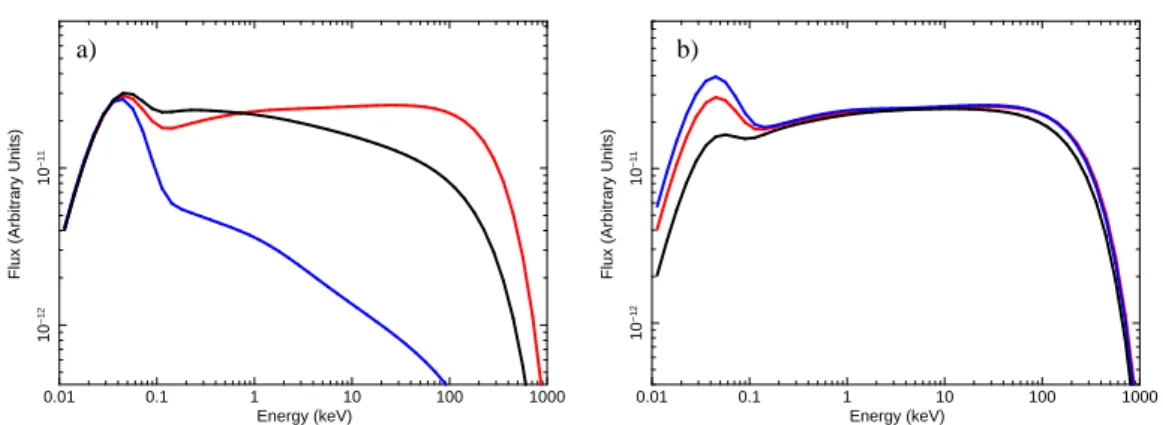
Fig. 2. a) Thermal comptonization spectra for the same plasma temperature and optical depth but
different geometry: blue: cylindrical, red: slab, black: spherical. b) We fix the plasma temperature but change its optical depth in order to have roughly the same spectral index in the 2-10 keV band. This exemplifies the ”geometrical” degeneracy of the thermal comptonization spectrum.
(Rybicki & Lightman, 1979)):
∆E E ≃ 4kTe mec2 ! + 16 kTe mec2 !2 for E ≪ kTe and N ≃ (τ + τ2) (1)
Then we define the Compton parameter
y = ∆E
E N. Large values of y means that the
Comptonization process is efficient and modi-fies noticeably the seed spectrum.
1.1.1. Thermal Comptonization spectrum
While thermal comptonization spectra have been computed since more than two decades, important effects like the anisotropy of the soft photon field were precisely taken into account in the beginning of the 90’s by the pioneering works of Haardt (1993); Stern et al. (1995) and Poutanen & Svensson (1996). These effects appear far from being negligible. Noticeably, for a given set of plasma temperature and opti-cal depth, the spectral shape is significantly dif-ferent for difdif-ferent disk-corona geometries (cf. Fig. 2a) but also for different viewing angle,
this last dependence being crucial for a cor-rect interpretation of X-ray spectra. These ef-fects underline the differences between realis-tic thermal comptonization spectra and the cut-off power law approximation generally used to mimic them. Moreover, the relation between the photon index Γ and the plasma tempera-ture and optical depth can be strongly degener-ated (”spectral” degeneracy) , different couples (τ, Te) giving, for the same disk-corona
geom-etry, the same Γ. A ”geometrical” degeneracy also exists and is exemplifies in Fig. 2b where the same high energy spectrum is reproduced with different set of parameters and with dif-ferent geometries. These degeneracies compli-cate the fitting procedure and high S/N data over broad band energy intervals are required to break them.
1.1.2. Radiative Balance
In a disk-corona system, the Comptonizing re-gion and the source of soft photons are
cou-pled, as the optically thick disk necessarily
re-processes and reemits part of the Comptonized flux as soft photons which are the seeds for Comptonization. The system must then satisfy equilibrium energy balance equations, which depend on geometry and on the ratio of di-rect heating of the disk to that of the corona.
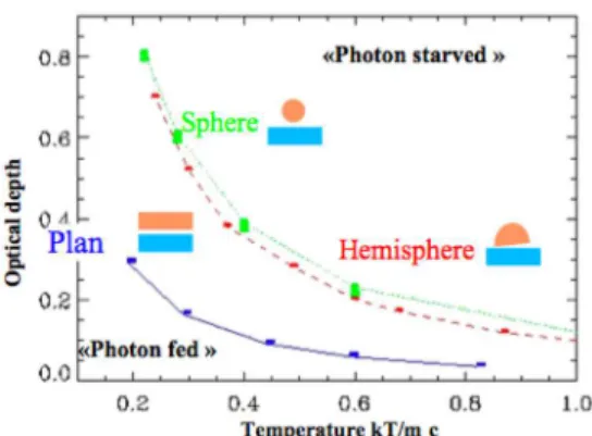
In the limiting case of a ”passive” disk (i.e. non intrinsically radiative, it radiates what it absorbs from the hot phase), the amplification of the Comptonization process, determined by the Compton parameter y, is fixed by geometry only (Haardt & Maraschi, 1991; Stern et al., 1995). Therefore, if the corona is in energy bal-ance, the temperature and optical depth must satisfy a relation which can be computed for different geometries of the disk+corona config-uration (cf. Fig. 3). It is then theoretically pos-sible to constrain the geometry of the system and verify the selfconsistency of the model, provided that the plasma temperature and op-tical depth Teand τ are known with sufficient
precision.
1.2. Non-thermal Comptonization In the case of non-thermal particles the energy transfert between the elctron and the photon is very efficient. For an electron with a Lorentz factor γ it is of the order:
∆E ≃ γ2E (2) Consequently the comptonization of a mo-noenergetic seed photon field by a non-thermal distribution of electrons n(γ) ∝ γ−s produces
Fig. 3. Different theoretical relationship,
cor-responding to different disk-corona geometry, between the corona temperature and optical depth in the case of energy balance between the hot and cold phases.
a non-thermal spectrum F(ν) ∝ ν− 2 (e.g.
Rybicki & Lightman 1979).
2. What can we expect with SIMBOL-X?
The comptonization process play a role in all SIMBOL-X science cases,
– AGNs (thermal comptonization in Seyfert
galaxies, non-thermal comptonization in Blazars)
– X-ray binaries (thermal comptonization in
the hard state, non-thermal(?) comptoniza-tion in the Intermediate and Soft states)
– X-ray background – Galaxy clusters – Supernovae remnants – GRBs
We detailed below some simulations of comp-tonization spectra showing the advances that we can expect with Simbol-X.
Fig. 4. Contour plots τ-kTefor simulations of different exposures (red: 1ks, blue: 5 ks and black: 50 ks). The simulated data correspond to a thermal comptonization spectrum with
L2−10keV = 10−11 erg.s−1.cm−2, kTe = 250
keV, τ = 0. Only the long exposure simulation enable to break the τ-kTedegeneracy
Petrucci: Models of Comptonization 285
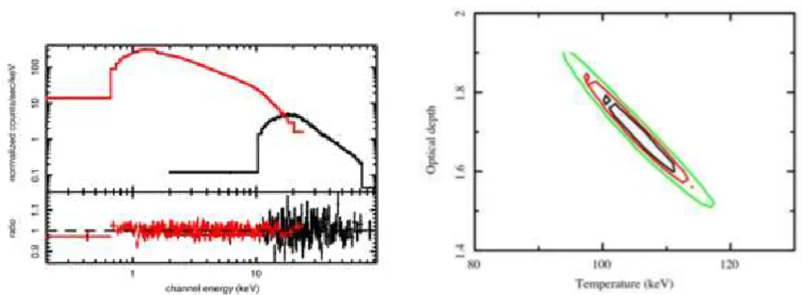
Fig. 5. Left: 500 sec. simulated Simbol-X data of Cyg X-1 assuming L2−10keV= 10−9erg.s−1.cm−2
kTe= 100 keV, τ = 1.7 and R = 0.3. Right: the corresponding τ-kTecontour plot.
2.1. Simu. N◦1: the case of a Seyfert galaxy
We simulate the spectrum of a Seyfert galaxy (NGC 5548) with different exposure time as-suming L2−10keV = 10−11erg.s−1.cm−2, kTe=
250 keV, τ = 0.1 and R = 1. We assume a slab geometry. Then we fit the faked data with the model used for the simulations. The corre-sponding contour plots τ-kTeare plotted in Fig.
4. If, for small exposure time (1 ks, red contour plot) the contour is very elongated, this ”spec-tral” degeneracy is broken for exposures of a few tens of ks (see the black contours that cor-respond to 50 ks). However we underline the fact that the real data generally show the pres-ence of complex reflection/absorption features that can strongly limit the data analysis and the precise study of the underlying continuum.
It is worth noting that a few tens of ks corresponds to the orbiting timescale at a few Schwarzschild radii around a 108solar masses black hole. It means that it should be possible with Simbol-X to follow the time evolution of the temperature and optical deth of the corona on a dynamical timescale. However simula-tions show that breaking the geometrical de-generacy will require very long (> 100 ks) ex-posure with Simbol-X.
2.2. Simu. N◦2: the case of a microquasar
We simulate the X-ray spectrum of the mi-croquasar Cyg X-1, with L2−10keV = 10−9 erg.s−1.cm−2 kT
e = 100 keV, τ = 1.7 and
R = 0.3. Good constraints of the spectral
pa-rameters can be obtained in a few hundred of seconds (cf. Fig. 5).
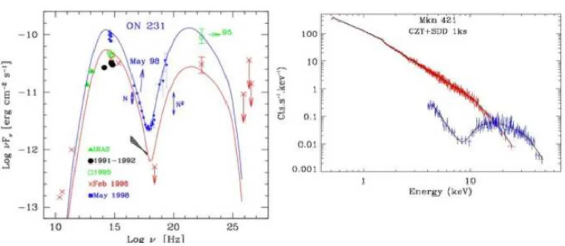
2.3. Simu. N◦3: the case of a blazar We also simulate the X-ray spectrim of the blazar Mkn 421 (cf. Fig. 6). The spectrum is very well determine in 1 ks ! But in order to have constrains on the Synchrotron Self-Compton process multi-λ observations (radio, Optical, IR, X and γ) are needed.
3. Conclusions
– Simbol-X should bring strong constrains
on comptonization spectra on dynamical time scale for AGNs, and on very short time scale in XrBs.
– However this can be complicated by the
presence of complex absorption/emission features
– The broadest energy range is needed
and multi-wavelength observations are rec-ommended (CTA, GLAST, HERSCHEL, ALMA, LOWFAR, WSO-UV, ...).
Fig. 6. Left: Typical Synchrotron Self-Compton spectrum of a blazar. Right: Simbol X simulation
of the blazar Mkn 421 in 1ks.
Acknowledgements. I am very grateful to the
CEA/DSM/DAPNIA/SAp for its financial support.
References
Haardt, F. 1993, ApJ, 413, 680
Haardt, F. & Maraschi, L. 1991, ApJ, 380, L51 Poutanen, J. & Svensson, R. 1996, ApJ, 470,
249
Rybicki, G. B. & Lightman, A. P. 1979, in A Wiley-Interscience Publication, New York: Wiley, 1979
Stern, B. E., Poutanen, J., Svensson, R., Sikora, M., & Begelman, M. C. 1995, ApJ, 449, L13+