HAL Id: hal-00679058
https://hal.archives-ouvertes.fr/hal-00679058
Submitted on 14 Mar 2012
HAL is a multi-disciplinary open access
archive for the deposit and dissemination of sci-entific research documents, whether they are pub-lished or not. The documents may come from
L’archive ouverte pluridisciplinaire HAL, est destinée au dépôt et à la diffusion de documents scientifiques de niveau recherche, publiés ou non, émanant des établissements d’enseignement et de
Non positive SVM
Gaëlle Loosli, Stephane Canu
To cite this version:
Non positive SVM
Gaëlle Loosli
1Stéphane Canu
2Research Report LIMOS/RR-10-16 1er octobre 2010
1. [email protected], LIMOS - Campus des cézeaux - 63173 Aubière
2. [email protected], LITIS - Technopôle - 76800 Saint-Etienne du Rou-vray
Abstract
Recent developments with indefinite SVM [11, 17, 5] have effectively demon-strated SVM classification with a non-positive kernel. However the question of efficiency still applies. In this paper, an efficient direct solver for SVM with non-positive kernel is proposed. The chosen approach is related to existing work on learning with kernel in Krein space. In this framework, it is shown that solving a learning problem is actually a problem of stabilization of the cost function instead of a minimization. We propose to restate SVM with non-positive kernels as a stabilization by using a new formulation of the KKT conditions. This new formulation provides a practical active set algorithm to solve the indefinite SVM problem. We also demonstrate empirically that the proposed algorithm outperforms other existing solvers.
Keywords: Non positive kernel, SVM solver
Résumé
La possibilité d’utiliser les SVM avec des noyaux non positifs a été démon-trée récemment avec les Indefinite SVM [11, 17, 5]. Toutefois la question de l’efficacité de la résolution se pose toujours. Dans cet article, nous proposons un algorithme efficace qui résout directement les SVM avec un noyaux non-positif. L’approche choisie est liée aux travaux existant sur l’apprentissage avec noyaux dans les espaces de Krein. Dans ce cadre, il est démontré que ré-soudre un problème d’apprentissage revient en fait à trouver un point stable de la fonction coût plutôt que le minimum. Nous proposons de reformuler les SVM avec noyaux non positifs comme une stabilisation en adaptant les conditions KKT. Cette nouvelle formulation permets de mettre en œuvre un algorithme de contraintes actives pour résoudre le problème des SVM indéfi-nis. Nous apportons également une preuve empirique de la supériorité de cet algorithme par rapport aux approches existantes.
Mots clés : Noyaux non positif, résolution de SVM
Acknowledgement / Remerciements
This work was supported in part by the IST Programme of the European Commu-nity, under the PASCAL2 Network of Excellence, IST-2007-216886. This publication only reflects the authors’ views. The authors also thank Ph. Mahey for helpful comments.
1
Learning with non positive kernel
From the first stages of SVM [15], non positive kernels are proposed and used, in particular the tanh kernel. In many application fields, some huge efforts are made to produce true Mercer kernels when the natural kernels turn out to be indefinite (for instance [7, 6]). Some author even study some kernels that are definite positive with high probability ([3]). However, until now, there is no adequate solver available. In [11], the authors propose to solve SVM with indefinite kernel considering that the indefinite kernel is a perturbation of a true Mercer kernel. They end up with a new optimiza-tion problem that is able to provide good soluoptimiza-tions. The major drawback however would be that the proposed algorithm requires to tune at least one more parameter, plus some different stopping criteria. Independently of the interest of this approach, it makes practical applications difficult. In [17, 5], the previous method is analyzed and improved. In [9], the author states that learning with indefinite symmetric kernels is actually consisting in finding a stationary point, which is not unique but each of those performs correct separation. Moreover, it is shown that the problem is then cannot be seen as a margin maximization although a notion of margin can be defined. We will see that similar notions appear in our formulation.
It has been shown ([13]) that learning with non positive kernel is actually solving the learning problem in a Krein space instead of a Hilbert space. It has also been shown that in this situation, the learning problem is not a minimization anymore but a stabilization problem. This means that the solution is a saddle point of the cost function. Applying this to SVM requires to interpret this stabilization setting. We first give the intuition behind the proposed method. Following [10], we start from the fact that a (unconstraint) quadratic program in a Krein space has a unique solution (if the involved matrix is non singular) which is in general a stationary point. In the case of SVM, we have to apply some box constraints that may exclude this unique solution. Moreover, the optimal constraint solution is not necessarily unique anymore.
In the definite positive case, solving the quadratic program under box constraints is a problem of projection of the unconstrained solution onto the admissible set. To do so, the gradient of the cost function gives the direction towards the minimum admissible point. In the indefinite case, this projection has to be redefined : indeed, since the optimal solution is not the minimum, we can not follow the gradient direction, which leads to the minimum. In our work, we propose another projection, in order to obtain the most stable point within the admissible set. In other words, we want the admissible point that has the lowest gradient.
In the next section, it is shown that the usual SVM problem with positive definite kernels can be directly extended to the indefinite case such that the provided solution is (one of) the most stable admissible point(s). In order to illustrate the fact that the proposed formulation is a stabilization, the original problem is modified such that any critical point becomes a local minimum. We point out that the optimal solution of the modified problem is the same as SVM with non positive kernels. Finally, the projection point of view is provided and it is shown that it also leads to the same problem. Having those three approaches, we conclude that the solution of a non positive SVM is the solution of a stabilization problem, which is also the projection of the unique unconstraint solution onto the admissible set, in the sense of the most stable point.
2
SVM and KKT conditions of optimality
Let’s consider a training set {X , Y} where xi ∈ X ∀i ∈ [1..n] are
exam-ples and yi ∈ Y are corresponding labels. In the case of binary classification,
possible values for labels are [−1; 1]. We denote K the symmetric kernel matrix, of size n × n. C is the hyper parameter, penalizing the training errors.
We recall in this section the SVM dual quadratic problem ([15]). This dual is obtained from the margin maximization formulation. A Lagrange multiplier αi is associated to each training example.
minα 12α⊤Gα− α⊤1 subject to α⊤y= 0 and 0 ≤ αi ≤ C ∀i ∈ [1..n] (1)
where G(i, j) = yiyjK(i, j).
We give the full KKT conditions for the classical SVM dual system (1). The KKT conditions of optimality are divided into stationarity condition, primal and dual admissibility and complementarity conditions. In the case of SVM dual, the stationarity condition is as follows:
α⊤G− 1⊤+ λy⊤− µ⊤+ η⊤ = 0 (2)
The primal admissibility is given by α⊤y= 0
αi ≤ C ∀i ∈ [1..n]
αi ≥ 0 ∀i ∈ [1..n]
The dual admissibility is given by
µi ≥ 0 ∀i ∈ [1..n]
ηi ≥ 0 ∀i ∈ [1..n]
(4) The complementary conditions are
αiµi = 0 ∀i ∈ [1..n]
(αi− C)ηi = 0 ∀i ∈ [1..n] (5)
Any solution respecting each of these conditions is a solution of the prob-lem. In the case the kernel matrix is definite positive, the dual SVM problem has a unique solution which is a global minimum.
2.1
Point of view 1 : the variational approach of quadratic
programming
In the case the kernel matrix is indefinite, the dual SVM problem is not well defined and the solution is not unique. Following [4] and the variational approach of quadratic programming, we can actually solve the problem using normal residuals (ie. solving Ax = b via A⊤Ax = A⊤b). Note that normal
equations could also be an option (ie. solving Ax = b via AA⊤x′ = b with
x= A⊤x′).
α⊤G = 1 − λy⊤+ µ⊤− η⊤
α⊤GG⊤ = (1 − λy⊤+ µ⊤− η⊤)G⊤ (6)
This can be seen as least squares. All the other conditions remain iden-tical.
2.2
Point of view 2 : a stabilization problem
Optimization technics provide minima and not saddle points. To that purpose, we propose to use a simple trick known as magnitude of the gradient, consisting in changing the problem such that any critical point becomes a local minimum. This is done computing the sum of the squares of the partial derivatives of the function to be stabilized. Let apply this to the following unconstrained function:
J = 1 2α
⊤Gα− α⊤1 (7)
Stabilizing J is equivalent to minimizing M:
M(α) =α⊤G− 1⊤, α⊤G− 1⊤
This provides the following system: minα α⊤G− 1⊤, α⊤G− 1⊤ subject to α⊤y= 0 and 0 ≤ αi ≤ C ∀i ∈ [1..n] (9)
Let now write the KKT condition of optimality for system (9). The stationarity condition is as follows:
(α⊤G− 1⊤+ λy⊤− µ⊤+ η⊤)G⊤= 0 (10)
The other condition are identical to eq. 3, 4 and 5. Those KKT conditions show that solving the SVM dual problem when the kernel is indefinite is actually a stabilization problem.
2.3
Point of view 3 : The projection
As already mentioned, the unconstraint problem has a unique solution. We want to project it onto the admissible set. However, this projection is not obvious : what is the closest point of the admissible set to the unconstraint optimum in the sense of the stabilization? We propose to define it as the most stable point, i.e. the admissible point minimizing the gradient of the cost function (which is α⊤G− 1⊤). Solving this minimization with the least
squares directly gives the same system as previously (eq. 9).
For illustration purpose, we draw the cost function for a sigmoid kernel of a simple 2 gaussians problem, obtained with two support vectors, for both CSVM cost and NPSVM cost. The plain area shows the admissible solutions. We can easily observe that the usual minimization technics would lead to a non optimal solution (see figure 1).
3
The solver
The proposed algorithm is derived from active set approach for SVM, sim-ilar to [16]. The sets of points are defined according to the complementarity conditions (see table 1).
By default, all training points are in the non support vector set I0 except
for a couple with opposite labels which is in Iw. Any other initial situation
Figure 1: SVM cost function with sigmoid kernel, illustrated for 2 support vectors. The plain area shows the admissible solutions. On the left, the CSVM cost function (eq. 1). On the right, the NPSVM cost function (eq. 10). The blue cross on each graph shows the solution computed by solving the usual CSVM problem. The red circle shows the solution proposed by the NPSVM.
Table 1: Definition of groups for active set depending on the dual variable values Group α η µ I0 0 0 >0 IC C >0 0 Iw 0 < α < C 0 0
3.1
Solving linear system in
I
wWe need to solve the linear system from the stationarity condition (eq. 10) only for unconstrained points, those of Iw. This leads to the following
equation :
α⊤(w)G(w,:)G(:,w) = (1(:)− λy⊤(:)− C1⊤(C)G(C,:))G(:,w)
This can be solved using QR decomposition of G, for which one can maintain a rank one update at each step of the algorithm. Computing λ can be easily done substituting α⊤
(w) in α⊤(w)y(w) = −C1⊤(C)y(C).
3.2
Activating constraints in
I
wIf any α(w)(i) does not lie in [0 C], the current solution is projected on
the admissible set such that all α(w)(i) satisfy the primal admissibility and
the violating point is transferred towards I0 or IC according to the violating
value.
3.3
Relaxing constraints in
I
0or
I
CIf the current solution is admissible, we check the stationarity conditions for I0 and IC (using eq. 10 and 5). The most violating point is transferred
from its group to Iw.
For any point j ∈ I0, µj >0 and ηj = 0. From eq. 10 :
(α⊤[w,C]G([w,C],:)− 1⊤+ λy⊤)G:,j >0
For any point k ∈ IC, µk = 0 and ηk >0. From eq. 10 :
(α⊤[w,C]G([w,C],:)− 1⊤+ λy⊤)G:,k<0
We can observe here that the notion of margin is distorted. Indeed, when using the same active set solver in the positive definite case, the margin clearly appears in the constraint relaxation (for j ∈ I0, the condition would be
α⊤
[w,C]G([w,C],j)+ λyj >1). This means that in the feature space, the solution
won’t have the same properties as the usual SVM, especially concerning the interpretation of support vectors relatively to the decision boundary.
3.4
The algorithm
1: Initialize (one random point for each class in Iw, all others in I0)
2: while solution is not optimal do 3: solve linear system (sec 3.1)
4: if primal admissibility is not satisfied then
5: project solution in the admissible domain : remove a support vector
from Iw (to I0 or IC) (sec 3.2)
6: else if stationarity condition is not satisfied then
7: add new support vector to Iw (from I0 or IC) (sec 3.3)
8: end if
9: end while
Note that the convergence after a finite number of step of the proposed algorithm can always be proved since it can be seen as an active set procedure applied to a convex QP and thus convergence proof in this case applies [12].
The code for proposed algorithm is available at ***.
3.5
Complexity
Compared to the same active set algorithm in the positive definite case, the proposed formulation increases the complexity. Let’s consider that only the original kernel is stored in memory, we list the added operations
– sec 3.1 : 2 matrix by matrix multiplication (O(n|Iw|2) and O(n2|Iw|))
– sec 3.2 : identical
– sec 3.3 : 1 matrix by matrix multiplication (O(n2(|I
0| + |IC|)))
These can be reduced by various strategies, such as caching, rank-one update, iterative search for violating example, etc.
4
Experimental results
In our experiements, we used the well known sigmoid kernel (tanh) : k(xi, xj) = tanh(scale×hxi, xji+bias) and the epanechnikov kernel (epanech)
: k(xi, xj) = max(0, 1−γ∗hxi, xji). We also used the positive gaussian kernel
4.1
UCI datasets
We tested our algorithm NPSVM on some popular UCI datasets [1] and compared the results to a usual SVM solution (refered as CSVM). For each scaled dataset (heart, sonar, breast cancer, diabetes) we provide the average test accuracy on 10 random split of the database. The statistically better results are bold and underlined (according to chi square independance test at level 2%) (see table 2).
Validation protocol
We describe here the protocol used for each dataset, inspired by [8]. The procedure is applied 10 times for each and the given results are on average.
– split randomly the dataset, 2/3 for cross validation, 1/3 for test. – perform 10 fold cross validation on the validation set
(C ∈ [0.01, 0.1, 1, 10, 100, 1000], σ ∈ [0.1, 0.5, 1, 5, 10, 15, 25, 50, 100, 250, 500]∗ √n
] for rbf kernel, scale = [pow2(−5 : 1.5 : 2), −pow2(−5 : 1.5 : 2)] and bias = [pow2(−5 : 1.5 : 2), −pow2(−5 : 1.5 : 2)] for tanh kernel). – train the svm on the full validation set with the parameters providing
the best average performance during cross validation. – test on the separate test set.
Table 2: Results on some UCI dataset.
Solver kernel Heart Sonar Breast C-SVM rbf 82.22% (23.2 sv) 84.78% (90.3 sv) 97.47% (53.8 sv) NPSVM rbf 83.44% (35.9 sv) 86.09% (94.9 sv) 97.37% (56.6 sv) NPSVM tanh 82.44% (14.8 sv) 84.06% (70.1 sv) 97.76 % (116 sv)
4.2
Usps digits
We tested the NPSVM on the well known USPS digits database. With kernel, tanh with scale = 0.004 and bias = −1.5, C = 100 we obtained 94.92% of good classification (1 vs 1 multiclass setting). With an epanech kernel (bandwidth = 0.01 and C = 1000) we obtained 94.07% of accuracy. Those experiments convinced us that this approach of non positive SVM could be applied at least to medium sized problem. However the tested non positive definite kernels did not outperform the positive definite ones on that problem.
Figure 2: Evolution of the cost function during training. Curves are scaled on vertical axis. On the left, we report the value of the usual CSVM cost function during training. On the right are curves corresponding to the modified cost function that is actually minimized. While the standard CSVM cost function decreases monotonically (rbf CSVM on the left graph), the cost function for NPSVM may increase. Note that test performance are similar for each of the reported experiment on this figure (dataset is synthetic data generated from the apple/banana setting).
4.3
Monitoring the cost function
We also observed the evolution of the cost function (eq 1) to illustrate the fact that the cost function is stabilized and not minimized (figure 2). However, we can observe that for some particular setting and datasets, the proposed algorithms may converge to a minimum.
4.4
Comparison to over solvers
libSVM
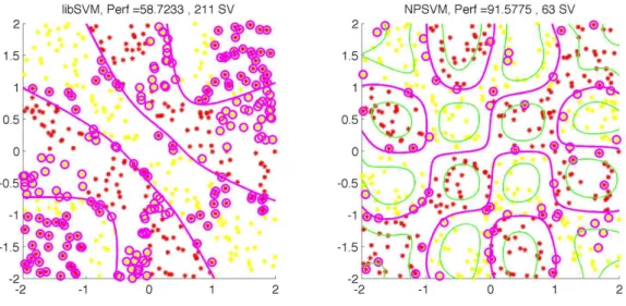
This part reports an experiment pointing out that the proposed approach can find much better solution than the widely used libSVM. Figure 3 illus-trates this on a synthetic problem of checkers. The sigmoid kernel is used, with positive scale and negative bias, as recommended in [14]. We can observe
that even though libSVM converges, the proposed solution poorly classifies the data while NPSVM converges towards a much better solution. Note that one can find some kernel parameters that works better for libSVM, but the reported result is frequent. Let us remark also that NPSVM is proposed
Figure 3: Results on checkers with NPSVM on the right and libSVM on the left, for an identical sigmoid kernel (scale = 1, bias = -1). Circles are support vectors.
here with an active set method but could also be implemented with an SMO approach.
IndefiniteSVM
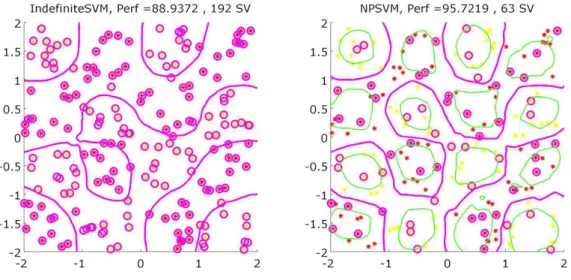
We conducted some experiments to compare our results to the Indefi-niteSVM toolbox ([11]). We show here one of the best results we manage to obtain (best in the sense of in favor of the indefiniteSVM). Note that we had difficulties to reach some good parameters for IndefiniteSVM. We can observe that even selecting favorable cases, IndefiniteSVM does not attain as good solutions as NPSVM. Moreover, those are usually less sparse.
Global comparison
From results in table 3, we can say that NPSVM clearly outperforms existing solvers handling non positive kernels. In terms of computational time, as expected the proposed implementation is slower than standard SVM solvers. However, it is much faster than IndefiniteSVM and can be used with medium size datasets.
Figure 4: Results on checkers with IndefiniteSVM on the left and NPSVM on the right, for an identical epanech kernel. Circles are support vectors.
5
Conclusion
In this article we present a new algorithm to solve SVM with non positive kernels. We base our work on the already stated fact that the solution, in this case, is a stabilized point and not a minimum, and we modified the solver according to that. We illustrate this point of view through three approaches, the variational point of view, the stabilization point of view and the projec-tion point of view. All leads to the same problem for which we provide a practical algorithm. Compared to a usual SVM solver, the NPSVM needs to take into account all training point for intermediate optimizations, thus the
Table 3: Comparison between IndefiniteSVM, libSVM and NPSVM on syn-thetic data, with the same kernel and C for all solvers . IndefiniteSVM is stopped after 2000 iterations if not converged
Solver Accuracy Training time Solution size Problem
IndefiniteSVM 58.25 % 16.34 s 48 sv Checkers 96 training points libSVM 48.56 % 0.003 s 52 sv tanh kernel NPSVM 84.82 % 0.35 s 28 sv min eig = -25.37 IndefiniteSVM 68.21% 726 s 496 sv Checkers 992 training points
libSVM 51.27% 0.01 s 232 sv tanh kernel NPSVM 90.84% 2.8 s 53 sv min eig = -136.07 IndefiniteSVM -% - s - sv Checkers 4992 training points
libSVM 53.30% 1.54 s 2369 sv tanh kernel NPSVM 92.41% 53.4 s 51 sv
-computational time is increased. To that point, we think some heuristics can be applied : a subset of points, chosen at random a priori, could be used in-stead of the whole training set to support the intermediate optimizations. An other lead consists in solving the linear program induced by the projection point of view, if we take norm 1 instead of least squares. This will be stud-ied in the near future. Let us note also recent work on projection in Krein space [2] that might be applied to the non positive kernels learning methods. Finally, we want to point out the fact that many well known technics, such as regularization paths, could easily be used for NPSVM.
References
[1] D.J. Newman A. Asuncion. UCI machine learning repository, 2007. [2] Tsuyoshi Ando. Projections in krein spaces. Linear Algebra and its
Applications, 431(12):2346 – 2358, 2009. Special Issue in honor of Shmuel Friedland.
[3] Sabri Boughorbel, Jean-Philippe Tarel, and Francois Fleuret. Non-mercer kernels for svm object recognition. In In British Machine Vision Conference (BMVC, pages 137–146, 2004.
[4] C. Brezinski. Projection methods for linear systems. J. Comput. Appl. Math., 77(1-2):35–51, 1997.
[5] Jianhui Chen and Jieping Ye. Training svm with indefinite kernels. In William W. Cohen, Andrew McCallum, and Sam T. Roweis, editors, ICML, volume 307 of ACM International Conference Proceeding Series, pages 136–143. ACM, 2008.
[6] Michael Collins and Nigel Duffy. Convolution kernels for natural lan-guage. In Thomas G. Dietterich, Suzanna Becker, and Zoubin Ghahra-mani, editors, NIPS, pages 625–632. MIT Press, 2001.
[7] Corinna Cortes, Patrick Haffner, and Mehryar Mohri. Positive definite rational kernels. In In Proceedings of The 16th Annual Conference on Computational Learning Theory (COLT 2003, pages 41–56. Springer, 2003.
[8] Tony Van Gestel, Johan A. K. Suykens, Bart Baesens, Stijn Viaene, Jan Vanthienen, Guido Dedene, Bart De, Moor, and Joos Vandewalle. Benchmarking least squares support vector machine classifiers. In Neural Processing Letters, pages 293–300.
[9] Bernard Haasdonk. Feature space interpretation of svms with indefinite kernels. IEEE Transactions on Pattern Analysis and Machine Intelli-gence, 27:482–492, 2005.
[10] Babak Hassibi and Ali H. Sayed andThomas Kailath. Indefinite-quadratic estimation and control: a unified approach to H2 and H [in-finity] theories, volume 16. 1999.
[11] R. Luss and A. d’Aspremont. Support Vector Machine Classifica-tion with Indefinite Kernels. Mathematical Programming ComputaClassifica-tions, 2009.
[12] Jorge Nocedal and Stephen J. Wright. Numerical Optimization. Springer, second edition, 2006.
[13] Cheng Soon Ong, Xavier Mary, Stéphane Canu, and Alexander J. Smola. Learning with non-positive kernels. In ICML ’04: Proceedings of the twenty-first international conference on Machine learning, page 81, New York, NY, USA, 2004. ACM.
[14] Hsuan tien Lin and Chih-Jen Lin. A study on sigmoid kernels for svm and the training of non-psd kernels by smo-type methods. Technical report, 2003.
[15] Vladimir Vapnik. The Nature of Statistical Learning Theory. Springer, N.Y, 1995.
[16] S. V. N. Vishwanathan, Alex J. Smola, and M. Narasimha Murty. Sim-plesvm. In ICML, pages 760–767, 2003.
[17] Yiming Ying, Colin Campbell, and Mark Girolami. Analysis of svm with indefinite kernels. In Y. Bengio, D. Schuurmans, J. Lafferty, C. K. I. Williams, and A. Culotta, editors, Advances in Neural Information Pro-cessing Systems 22, pages 2205–2213. 2009.