A climatology of surface ozone in the extra tropics: cluster analysis of observations and model results

(1)

HAL Id: hal-00303071

https://hal.archives-ouvertes.fr/hal-00303071

Submitted on 23 Aug 2007

HAL is a multi-disciplinary open access

archive for the deposit and dissemination of sci-entific research documents, whether they are pub-lished or not. The documents may come from teaching and research institutions in France or abroad, or from public or private research centers.

L’archive ouverte pluridisciplinaire HAL, est destinée au dépôt et à la diffusion de documents scientifiques de niveau recherche, publiés ou non, émanant des établissements d’enseignement et de recherche français ou étrangers, des laboratoires publics ou privés.

A climatology of surface ozone in the extra tropics:

cluster analysis of observations and model results

O. A. Tarasova, C. A. M. Brenninkmeijer, P. Jöckel, A. M. Zvyagintsev, G. I.

Kuznetsov

To cite this version:

O. A. Tarasova, C. A. M. Brenninkmeijer, P. Jöckel, A. M. Zvyagintsev, G. I. Kuznetsov. A climatology of surface ozone in the extra tropics: cluster analysis of observations and model results. Atmospheric Chemistry and Physics Discussions, European Geosciences Union, 2007, 7 (4), pp.12541-12572. �hal-00303071�

(2)

ACPD

7, 12541–12572, 2007

A climatology of surface ozone in the

extra tropics O. A. Tarasova et al. Title Page Abstract Introduction Conclusions References Tables Figures ◭ ◮ ◭ ◮ Back Close

Full Screen / Esc

Printer-friendly Version Interactive Discussion

Atmos. Chem. Phys. Discuss., 7, 12541–12572, 2007 www.atmos-chem-phys-discuss.net/7/12541/2007/ © Author(s) 2007. This work is licensed

under a Creative Commons License.

Atmospheric Chemistry and Physics Discussions

A climatology of surface ozone in the

extra tropics: cluster analysis of

observations and model results

O. A. Tarasova1,2, C. A. M. Brenninkmeijer1, P. J ¨ockel1, A. M. Zvyagintsev3, and G. I. Kuznetsov2

1

Max Planck Institute for Chemistry, Mainz, Germany 2

Lomonosov Moscow State University, Faculty of Physics, Moscow, Russia 3

Central Aerological Observatory, Dolgoprudny, Russia

Received: 6 July 2007 – Accepted: 22 August 2007 – Published: 23 August 2007 Correspondence to: O. A. Tarasova (tarasova@mpch-mainz.mpg.de)

(3)

ACPD

7, 12541–12572, 2007

Full Screen / Esc

EGU

Abstract

Important aspects of the seasonal variations of surface ozone are discussed. The un-derlying analysis is based on the long-term (1990–2004) ozone records of Co-operative Programme for Monitoring and Evaluation of the Long-range Transmission of Air Pol-lutants in Europe (EMEP) and the World Data Center of Greenhouse Gases which 5

do have a strong Northern Hemisphere bias. Seasonal variations are pronounced at most of the 114 locations for any time of the day. Seasonal-diurnal variability classifica-tion using hierarchical agglomeraclassifica-tion clustering reveals 5 distinct clusters: clean/rural, semi-polluted non-elevated, semi-polluted semi-elevated, elevated and polar/remote marine types. For the cluster “clean/rural” the seasonal maximum is observed in April, 10

both for night and day. For those sites with a double maximum or a wide spring-summer maximum, the one in spring appears both for day and night, while the one in summer is more pronounced for daytime and hence can be attributed to photochemical pro-cesses. For the spring maximum photochemistry is a less plausible explanation as no dependence of the maximum timing is observed. More probably the spring maximum 15

is caused by dynamical/transport processes. Using data from the 3-D atmospheric chemistry general circulation model ECHAM5/MESSy1 covering the period of 1998– 2005 a comparison has been performed for the identified clusters. For the model data four distinct classes of variability are detected. The majority of cases are covered by the regimes with a spring seasonal maximum or with a broad spring-summer maxi-20

mum (with prevailing summer). The regime with winter–early spring maximum is repro-duced by the model for southern hemispheric locations. Background and semi-polluted sites appear in the model in the same cluster. The seasonality in this model cluster is characterized by a pronounced spring (May) maximum. For the model cluster that covers partly semi-elevated semi-polluted sites the role of the photochemical produc-25

tion/destruction seems to be overestimated. Taking into consideration the differences in the data sampling procedure the carried out comparison demonstrates the ability of the model to reproduce the main regimes of surface ozone variability quite well.

(4)

ACPD

7, 12541–12572, 2007

Full Screen / Esc

1 Introduction

Ozone is a key species of tropospheric chemistry, polluted or pristine (Crutzen, 1973; Fabian and Pruchniewz, 1977), and it is a greenhouse gas (IPCC, 2006). Surface ozone is of special concern as an air pollutant. Particularly, despite the measures taken to ameliorate surface ozone increases by reducing precursor emissions (Ord ´o ˜nez et al., 5

2005; Vingarzan, 2004; Oltmans et al., 2006), its levels appear to increase. Jonson et al. (2006) suggested that reductions in regional production were annulled by increasing levels of background ozone, thus leading to the upwards trend observed at Mace Head in Ireland. Even over parts of the Atlantic Ocean ozone has been increasing (Lelieveld et al., 2004), attributed to increase in anthropogenic NO_x emissions in Africa. At the 10

same time at certain locations surface ozone trends can be negative (Tarasova et al., 2003; Vingarzan, 2004). Altogether a deeper understanding of ozone, of its spatial variability, its temporal variations, trends and ultimately its budget are still required. The diversity of the processes that control and affect tropospheric ozone combined with its variable rather short lifetime produce a most complex system. Careful analyses 15

of the many observations of this interesting gas contribute to our understanding as do increasingly model simulations. In this paper we will combine both approaches for better understanding extra-tropical ozone and first briefly review the current status.

Surface ozone over the continents has a pronounced seasonal cycle (e.g. Tropo-spheric Ozone Research, TOR-2 final report; Zvyagintsev, 2004). The shape of this 20

cycle depends primarily on the latitude (insolation), on the availability of precursors (chemistry) and also on the altitude (temperature, mixing, downward transport, pre-cursors). The maximum can occur in winter/early spring (Oltmans et al., 2004, 2006, 2007; Gros et al., 1998; Scheel et al., 1990), in spring, or in spring/summer (Scheel et al., 1997; Felipe-Soteloa et al., 2006; Scheel, 2003; Schuepbach et al., 2001; Varotsos 25

et al., 2001; Sunwoo and Carmichael, 1994; Ahammed et al., 2006, and many other papers). A complex interplay of photochemical and dynamical processes controls the main features of surface ozone variability (Lelieveld and Dentener, 2000) and the shape

(5)

ACPD

7, 12541–12572, 2007

Full Screen / Esc

EGU

of the seasonal cycle (Oltmans et al., 1992; Monks, 2000). An earlier classification of the surface ozone seasonal cycles for European sites was performed by Esser (1993) and confirmed by the results of the TOR-2 project. This classification was based on a priori information on the pollution and local meteorological conditions at the observa-tional site and hence can be considered to have some degree of subjectivity. Moreover, 5

it was noted that even for neighboring locations the shape of the seasonal variations can be different (e.g. Felipe-Soteloa et al., 2006).

A prominent feature, namely the spring maximum at Northern Hemisphere mid-latitudes that is well visible at background observatories is still subject to research (Scheel et al., 1997; EMEP Assessment, 2004; Schuepbach et al., 2001; Li et al., 10

2002). A re-analysis of historical records confirms the existence of the spring maxi-mum in earlier years (Linvill et al., 1980; Monks, 2000; Nolle et al., 2005), although clearly the shape of the cycle is sensitive to pollution conditions. For example, Zvya-ginsev (2004) analyzing the 1976–1995 Hohenpeissenberg data (for which spring and summer maxima are separated) showed that the summer maximum changes stronger 15

than the spring maximum. Scheel et al. (2003) reported that at the Zugspitze for more polluted years the seasonal maximum is observed later in the year.

Most of the aspects of the surface ozone seasonality, and its spring maximum in particular, can be found in the review of Monks (2000). He mentions a number of issues that need further work, namely the relative contributions of dynamical (STE) 20

and photo-chemical processes, the relationship between ozone and precursor cycles, and the role of long-range transport versus in-situ photochemical production.

Whereas most overview papers consider the seasonal cycle on the basis of a pri-ori information for given observation sites, our contribution to better understanding the surface ozone seasonality is solely centered on a statistical analysis of time series and 25

of model output. We use data from the extra-tropics around the globe to gain insight into average seasonal and diurnal changes, thereby trying to attribute the roles of rel-evant underlying processes. Unlike most studies we do include the diurnal cycle into our considerations. This point is very important as diurnal variability bears information

(6)

ACPD

7, 12541–12572, 2007

Full Screen / Esc

on local pollution conditions and boundary layer dynamics. In particular, the rate of the afternoon ozone growth is defined by the local precursors level, formation of the morning minimum is defined by the properties of the underlaying surface and intensity of the temperature inversion. Moreover, formation of the breeze-type (with morning di-urnal maximum) or mountain-type (with night didi-urnal maximum) shape of didi-urnal cycle 5

is defined by dynamics of the boundary layer. So, the inclusion of diurnal variations into analysis can help more clearly distinguish different regimes of the surface ozone variability and identify the processes driven by sunlight. After applying a non-biased statistical approach to observations, we do virtually the same to model output.

Our paper has the following structure. In Sect. 2 we discuss observational data 10

used for analysis and give a brief overview of the ECHAM5/MESSy1 modeling system. In Sect. 3 the analytical technique is discussed and Sect. 4 presents the results of classification of the observational data and model output, gives interpretation of the obtained results and classes intercomparison. Conclusions are presented in Sect. 5.

2 Data

15

For our climatological study we use surface ozone records of at least 10 years duration from non-tropical latitudes (excluded is the belt between 25◦_{S and 25}◦_{N). The hourly}

data were downloaded from the EMEP project (http://www.emep.int) and the World Data Center for Greenhouse Gases websites (http://gaw.kishou.go.jp). A total of 114 time series is used. Because the majority of the datasets is obtained from EMEP the 20

total data set has a geographical bias to Europe. For the Southern Hemisphere where the measurement coverage is very poor, some 8 year records had to be used. The data are presented in nmol/mol. The entire set of sites is listed in Table 1 including site coordinates, altitude, identifier and cluster membership defined as described below. All of the used datasets have confirmed quality (ex., Hjellbrekke and Solberg, 2003). 25

Variability of the monthly mean mixing ratio calculations (annual standard deviation of the monthly means for each hour of the day) is estimated to be between 2% and 7%

(7)

ACPD

7, 12541–12572, 2007

Full Screen / Esc

EGU

(Zvyagintsev, 2004) for each particular location.

The comparison with model output is performed using the results of the 3-D atmospheric chemistry general circulation model ECHAM5/MESSy1 (http://www.

messy-interface.org), which – in the applied setup – simulates consistently the chem-istry and dynamics of the atmosphere between the Earth’s surface and the upper 5

stratosphere/lower mesosphere (approx. 80 km). The data used here are the results of the S1 simulation presented by J ¨ockel et al. (2006). In this simulation the model dynamics has been weakly nudged in the free troposphere/lower stratosphere (up to 100 hPa) towards ECMWF operational analysis data, in order to follow the actual me-teorology. For our analysis it is important to mention that most of the ozone precursors 10

emissions have been prescribed for each year as monthly average fluxes using the year 2000.

The provided model output has a time resolution of 5 h, yielding an hourly resolved diurnal cycle every 5 days. From the 2.8◦

×2.8◦gridded model output ozone time series at the position of the observational sites have been sub-sampled. Due to the rather 15

coarse model grid, some neighboring sites are located in the same model grid box. They are taken into consideration once only. Thus, the number of the used model time series (72) is smaller than the actual number of sites (114) which are used for the analysis. The model output covers the period from 1998 to 2005 and does not overlap completely with the measurement period. In addition to the ozone time series, also 20

the simulated stratospheric ozone tracer (O(s)₃ ) has been sampled (available from 2000 onward) in the same way. This tracer indicates the ozone content that originates from the stratosphere. In the analysis this information is used to estimate the contribution of the STE to the observed seasonal-diurnal variations of the surface ozone. At the same time it should be kept in mind that the periods of averaging are different and obtained 25

(8)

ACPD

7, 12541–12572, 2007

Full Screen / Esc

3 Statistical analysis

Long-term trends of surface ozone mixing ratios can differ from site to site (e.g. in the range from +2.6±0.6%/year to −1.4±0.7%/year as reported by Virgarzan, 2004), which increases the uncertainty in the estimated means. To reduce possible biases and to unify the datasets all original time series were first de-trended by subtracting the 5

incline of a time linear regression. This provides statistical uniformity of the seasonal variations, i.e. the averaging for each yearly period should gives the same mean within the range of uncertainties. The trend correction was between −0.8 nmol/mol a year and +1.4 nmol/mol a year. The question of the trends signature is a topic of another paper.

10

For each particular location (measurement site or corresponding model grid cell) 24 averaged over measurement period seasonal cycles were derived representing each hour of the day for the whole measurements/simulation period. The result is a matrix giving the average seasonal variation for a given time and the diurnal cycle for each month simultaneously, O_3,i (h, m). Here i is the index of the measurement/simulated 15

data location, h is local time in hours and m is month of a year. For obtaining temporal uniformity, data for the Southern Hemisphere were shifted by 6 months.

The term “cluster analysis” (first used by Tryon, 1939) comprises a number of differ-ent algorithms and methods for grouping objects with similar properties into respective groups in a way that the degree of association between two objects is maximal if they 20

belong to the same group and minimal otherwise. Given the above, cluster analysis can be used to discover structures in data without a priori information on the data properties (Hill and Lewicki, 2006).

Basically there are two different algorithms applied in the clustering (Everitt, 1993), namely hierarchical and non-hierarchical. The difference can be found in various text 25

books, and a brief description in Beaver and Palazoglu (2006). The purpose of the hierarchical clustering is to join objects into successively larger clusters, using some measure of similarity or distance. A detailed overview of hierarchical classification

(9)

(in-ACPD

7, 12541–12572, 2007

Full Screen / Esc

EGU

cluding agglomeration and discrimination techniques) can be found in Gordon (1987). Hierarchical clustering is for instance often used in air transport classification (Cape et al., 2000; Colette et al., 2005).

The agglomeration hierarchical procedure begins by initializing N singleton clusters (in our case one seasonal-diurnal matrix). Then the two closest clusters are merged to 5

form a single cluster. This process is repeated until one cluster remains. Results of the agglomeration process can be different depending on the methods used to evaluate the dissimilarities (similarities) or distances between objects when forming the clusters and the measures of these distances.

In this paper a squared Euclidean distance is used as a measure of distance between 10

the objects:

dist2(O_3,i,O_3,j) =X h,m

(O_3,i(h, m) − O3,j(h, m))2. (1)

As an agglomeration rule the average linkage within groups is used. It takes into con-sideration the mean distance between all possible inter- or intra-cluster pairs, unlike the average linkage method (Beaver and Palazoglu, 2006), where only the distance 15

between clusters is taken into consideration. The average distance between all pairs in the resulting cluster is made to be as small as possible, min(d_{i i}, d_{j j}), while the average distance between all the pairs in two different clusters should be maximized, max(di j):

d(i , j ) = _n1 inj ni P s=1 nj P m=1 dist2(O_3,s,O_3,m), (2)

where n_i and n_j are the number of the objects in the clusters i and j . As far as we 20

have a rather small number of objects, the application of this agglomeration method allows us obtaining the most homogeneity within clusters. In spite of the fact that the best results can be obtained with the Ward method, it is not applicable in our case as it tends to force the clusters to have similar sizes, which is unlikely in the case of spatially non homogeneous information.

(10)

ACPD

7, 12541–12572, 2007

Full Screen / Esc

In the agglomeration process the total distance between cluster centers and cluster members is determined at each step, representing a total dispersion S of the system

S(n_i) = ni X i =1 nj X j =1 dist2(O_3,j,O_3,i), (3)

where O_3,i is a center of the cluster i , O_3,j are the members of the cluster i , nj is a number of the elements in the cluster i and n_i is a number of clusters. The dispersion 5

S rises monotonously and reaches its maximum if all the vectors are unified in a single cluster. The choice of the appropriate number of clusters is determined by the point of the extreme growth rate of S. At the same time there is still freedom in the choice of the cluster numbers and the agglomeration procedure can be interrupted at any step.

Unlike the hierarchical clustering procedure, applied here, non-hierarchical clustering 10

(e.g., the k-means algorithm) supposes that the number of clusters is already known and that the objects are distributed between the discrete numbers of the groups (Moody et al., 1991). This algorithm is widely used in those cases where a priori information on the nature of the measurements is available. An example is the classification of aerosol types (Omar et al., 2005). Since we have no a priori information on the number of the 15

particular patterns in our data this method is not applicable here.

As stated we apply hierarchical agglomeration clustering to the seasonal-diurnal ma-trices of the measurements and of the model output. The optimal number of observa-tional clusters (OC) was found to be 5 and the optimal number of model clusters (MC) appeared to be 4. The cluster membership was defined at the corresponding step 20

and the average mixing ratios (cluster centers) and their standard deviation for the seasonal-diurnal cycle in each cluster were calculated. The procedure was applied to the measurements and to the simulated data independently.

(11)

ACPD

7, 12541–12572, 2007

Full Screen / Esc

EGU

4 Results

4.1 Classes of measured surface ozone seasonal-diurnal cycles

The 5 typical classes identified by cluster analysis of the average seasonal-diurnal ma-trices of 114 sites are visualized in Fig. 1. The characteristics of the obtained clusters as well as their comparison with the model output classification are summarized in 5

Table 2.

Cluster 1 (Fig. 1a) referred to as OC1 (Observational Cluster 1) is characterized by a pronounced spring maximum (April). The timing of the seasonal maximum does not depend on the time of the day (Fig. 2). The maximum amplitude (difference between daily maximum and daily minimum) of the diurnal cycle is observed in August (up to 10

7.0 nmol/mol), which is rather small and may be explained by a combination of late summer chemistry (decaying plant material, higher temperatures, still high insolation) and boundary layer dynamics (colder nights with stronger inversions and hence en-hanced deposition at the surface). It can be seen (Fig. 1a) that in OC1 night/early morning mixing ratios in August are the lowest. The maximum amplitude of the sea-15

sonal variations is observed close to the time of the diurnal minimum (17 nmol/mol). It should be mentioned that the variability of the seasonal amplitude for the different hours is less than 20% of its maximal magnitude. Such a regime of surface ozone variability is often reported for non-polluted/rural sites not only in the extra tropics (e.g. Scheel et al., 1997; EMEP Assessment, 2004; Oltmans et al., 2006; Sunwoo et al., 1994) but 20

also at some tropical locations (Ahammed et al., 2006). A comparison of the properties of OC1 with literature data indicates that sites in this cluster are unpolluted/remote and could be considered as representative for background conditions. Indeed, plotting the sites of this cluster on the map (Fig. 3) and consulting the sites coordinates in Table 1 confirm this result.

25

A more complex shape of the cluster averaged seasonal-diurnal variability is ob-served in OC2 (Fig. 1b). At night the seasonal cycle is characterized by a pronounced spring maximum in April, which is shifted to May for daytime hours (Fig. 2). A

(12)

sec-ACPD

7, 12541–12572, 2007

Full Screen / Esc

ondary seasonal maximum is formed in August during a day. The spring maximum of OC2 is lower than that for the unpolluted OC1 at night (up to 9.0 nmol/mol) while during daytime the value of the spring maximum for OC2 (for example at 16 h) even exceeds the value of the spring maximum in OC1 (up to 2.0 nmol/mol). This probably points to higher photo-chemical ozone production in OC2 in comparison with OC1 as 5

far as higher values are observed in OC2 only during daytime. Assuming that OC2 is more polluted than OC1, the lower seasonal maximum at night may be also explained by ozone destruction through reaction with NO_x. This is supported by the highest differences between the clusters which are observed for the winter months. Seasonal variations similar to the ones in OC2 have been reported for non-elevated semi-polluted 10

and even for urban sites (e.g. Varotsos et al., 2001). The maximum amplitude of the diurnal cycle of OC2 is observed in August (up to 21 nmol/mol) and that of the seasonal cycle is observed at 16:00 h local time (26 nmol/mol). These characteristics of the OC2 seasonal-diurnal variability in comparison with literature information (TOR-2 Final Re-port, 2003; Fiore et al., 2003; Felipe-Soteloa et al., 2006; Monks, 2000) suggest that 15

the surface ozone regime presented by this cluster is characteristic for semi-polluted non-elevated sites. It should be mentioned that for some sites included in this cluster (e.g. IT0004R, KPS646N00, and some others) the value of the summer maximum can exceed the spring maximum especially for daytime hours, confirming the photochem-ical nature of the summer maximum. The locations of the sites of OC2 on the map 20

(Fig. 3) show that they may be affected by a variety of pollution sources.

OC3 (Fig. 1c) is characterized by a pronounced winter seasonal maximum (December–January). This corresponds to June–July in the Southern Hemisphere, which is a winter season. Southern hemispheric data were 6 months shifted prior to analysis. Winter seasonal maximum is observed at any time of the day and in absence 25

of diurnal variations (Fig. 2). Such a shape of the seasonal cycle is reported for the majority of the mid- and high-latitude locations of the Southern Hemisphere, in partic-ular for Cape Point, Cape Grim, South Pole and others (Oltmans et al., 2006, 2007; Scheel et al., 1990; Gros et al., 1998). The diurnal variability in this cluster is very

(13)

ACPD

7, 12541–12572, 2007

Full Screen / Esc

EGU

weak and does not exceed 1 nmol/mol. The absence of the diurnal variability for this cluster indicates that the surface ozone variations are controlled by the processes with time-scales longer than a day. The maximum amplitude of the seasonal cycle in OC3 reaches 14.0 nmol/mol. The high stability of OC3 probably shows that the main mech-anism affecting local surface ozone variability is atmospheric transport. The regime 5

of the surface ozone variability, characteristic for OC3, can take place at the locations where photochemical activity is weak because of low precursor levels and/or because of the low levels of sunlight and/or because chemical destruction does not play a role in winter (like in polar regions or on remote islands). Consulting the map of the site dis-tribution in the different clusters (Fig. 3) we can see that OC3 is represented by only 4 10

sites, situated in the polar (or close to polar) coastal zones of Antarctica, New Zeeland and Alaska. The seasonal maximum at these locations can be explained by transport process, both vertical motion (STE) and horizontal advection with weaken chemical ozone production/destruction.

The mean seasonal-diurnal cycle in the observational cluster 4 (OC4, Fig. 1d) is 15

characterized by a broad spring-summer maximum with higher night values. At night the maxima are not distinguishable (Fig. 2), while during the day it is possible to ob-serve the double peak structure. The mixing ratios obob-served in OC4 exceed those in the other clusters at any season and any time of the day. The maximum amplitude of the diurnal cycle is observed in June–July in the period of the highest insolation 20

and it reaches 6.0 nmol/mol. This value is substantially lower than in the other clusters except for OC3, where the diurnal cycle is absent. Since the maximum is formed at night, the diurnal cycle can be driven by boundary layer dynamics, while photochemi-cal production only plays a minor role. The maximum amplitude of the seasonal cycle is observed between 09:00 p.m. and 12:00 p.m. (up to 18.0 nmol/mol). Rather stable 25

high mixing ratios, nearly insensitive to the time of the day with a slight growth at night can correspond to the surface ozone regime observed at mountain sites (Oltmans at al., 2006; Fiore et al., 2003; Scheel et al., 2003; Schuepbach et al., 2001; Tarasova et al., 2003). Presenting OC4 on the map indeed shows elevated locations (Fig. 3). The

(14)

ACPD

7, 12541–12572, 2007

Full Screen / Esc

summary in Table 2 shows that there are 6 locations included in OC4 and all of them are above 1700 m a.s.l. (Table 1).

OC5 (Fig. 1d) has a structure of the seasonal-diurnal cycles similar to that of OC2. Notwithstanding, the ozone levels in OC5 are higher than in OC2 during any season and during any time of the day (Fig. 2). Since this holds in winter and at night, it is 5

plausible that the sites of this cluster are either less polluted (with less chemical de-struction of ozone) or more elevated. In OC5 the spring maximum is dominating at night, while during the day the summer maximum is pronounced and comparable to the spring one (Fig. 2). The spring maximum in OC5 is one month delayed in compar-ison with the background OC1, pointing to the higher pollution level for OC5. Similar 10

effect was reported by Scheel et al. (2003), who showed that at the Zugspitze for more polluted years the seasonal maximum is shifting to later months. The maximum am-plitude of the diurnal cycle in OC5 is observed in August and reaches 11.0 nmol/mol, which is nearly by a factor of 2 lower than in OC2. This means that either daily ozone production plays a less important role in OC5 in comparison to OC2 or that the diurnal 15

variability in OC5 is less sensitive to the diurnal changes of the vertical mixing. The comparison of the altitude ranges of sites represented in OC2 and OC5, respectively, shows that the first group (1 m–1302 m a.s.l., average 225 m a.s.l.) is less elevated than the second group (105–2008 m, average of 952 m a.s.l.). The maximum ampli-tude of the seasonal variations in OC5 is observed at 04:00 p.m. and reaches the 20

value of 28.0 nmol/mol. Summarizing the discussed features of OC5 and comparing them with the properties of the seasonal cycles in various publications (Oltmans at al., 2006; Fiore et al., 2003; Scheel et al., 2003) it is possible to conclude that OC5 should represent the semi-polluted semi-elevated sites. This is confirmed inspecting Fig. 3. 4.2 Classes of model simulated surface ozone seasonal-diurnal cycles

25

To compare the features of the clusters obtained for the measurement sites with the results from the global model simulation, we applied the same technique to the sampled model output at the grids covering the measurements locations. For the model results,

(15)

ACPD

7, 12541–12572, 2007

Full Screen / Esc

EGU

the hierarchical clustering procedure carried out as described before revealed only 4 distinct clusters unlike the 5 for the observations. It should be noted (see Table 2 for details) that the majority of the grid cells are covered by 2 big clusters, while one of the regimes is represented by two grid cells only.

Similar to the measurements, the mean seasonal-diurnal cycles of the model clus-5

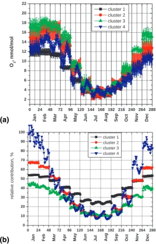
ters (MC) are presented in Fig. 4. As additional information used for the interpretation of the variability, the mean stratospheric contribution calculated for each model cluster is presented (Fig. 5). This parameter is used to indicate the role of stratosphere-to-troposphere transport and its changes throughout the year for the seasonal-diurnal cycles represented by the model clusters. Figure 5a gives stratospheric contribution 10

in absolute values, while Fig. 5b shows it as a relative contribution (in percent of the average simulated mixing ratios). As expected the maximum of the stratospheric con-tribution in absolute values is observed in spring (Fig. 5a).

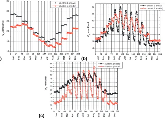
Comparison of the main properties of the observational clusters and the ECHAM5/MESSy1 model clusters respectively (Figs. 1 and 4), shows that the model 15

reproduces the main classes of the observed variability reasonably well. The follow-ing classes are represented by the model: a cluster with winter-early sprfollow-ing seasonal maximum and less pronounced diurnal cycle (analogous to OC3), a cluster with spring maximum and developed diurnal cycle (analogous to OC1 and OC2), a cluster with elevated mixing ratios (throughout the year), pronounced seasonal spring maximum 20

and slight night concentration increase, and a fourth cluster with a developed seasonal maximum in summer and a strong diurnal cycle.

The model cluster MC1 (Fig. 4a) by its properties looks rather similar to OC3. Pre-senting OC3 and MC1 together (Fig. 6a) highlights that for the period from May till August the difference between the mixing ratios in these two clusters is less that 25

5 nmol/mol. The strongest difference is observed in autumn and winter, but still the model exceeds the observations by less than 8 nmol/mol. It is interesting to note that for the time of the strongest discrepancy the stratospheric relative contribution in the model is up to 55% (Fig. 5b). Analyzing the geographical distribution of the grid cells

(16)

ACPD

7, 12541–12572, 2007

Full Screen / Esc

with this particular regime we find only Southern Hemispheric locations. In total there are only 6 grid-boxes included in MC1 covering 3 locations (of 4) representative for the similar regime in the measurements. Thus, it can be concluded that the variability of the surface ozone at remote locations, taking into consideration the limitations of the model setup, is captured by the model reasonably well. A possible reason for the 5

observed discrepancy can be an overestimated stratospheric contribution in the model. MC2 covers the majority of the grid cells taken into consideration (43 of 72). The average seasonal-diurnal cycle in this cluster presented in Fig. 4b is characterized by the pronounced spring maximum in May. This coincides with the timing of the sea-sonal maximum in OC2 (Fig. 6b). The average levels of the mixing ratios are in a good 10

agreement between OC2 and MC2, but the diurnal variability represented by the model is much smaller in MC2 compared to the observations, reaching 10 nmol/mol in June. This value is close to the amplitude of the diurnal variability in OC1, which represents background conditions. It is likely that MC2 represents an average regime between semi-polluted (less diurnal variability) and background (less average concentrations) 15

conditions. In MC2 the maximum relative stratospheric contribution is observed for winter months reaching about 68%, while this value does not exceed 15% for summer months (Fig. 5b). As far as there is no seasonality in the observed difference between MC2 and OC2 the stratospheric contribution for this model cluster appears to be cor-rect. Taking into account the rather coarse model resolution, the obtained agreement 20

can be considered as reasonable. Figure 3 shows, that MC2 covers most of the loca-tions in the mid latitudes of the USA including the elevated site Niwot Ridge, Northern and Central Europe and Japan. As it was discussed above for the measurements, these sites are mostly represented by OC1 and OC2.

The model cluster 3 (MC3) is represented by two grid-boxes only. The average 25

seasonal-diurnal variability in this cluster is presented in Fig. 4c and it is characterized by high (higher in average than all the other model clusters) mixing ratios with a rather broad spring maximum while the seasonal minimum is observed in July. The diurnal cycle in MC3 is rather weak reaching its maximum in August (3.7 nmol/mol). It is likely

(17)

ACPD

7, 12541–12572, 2007

Full Screen / Esc

EGU

that in this cluster the surface ozone is controlled by the processes with time-scales longer than a day. As far as a slight increase in the concentration occurs for evening hours and seasonality is characterized by the spring maximum only, this regime is characteristic for unpolluted locations with weak boundary layer photochemistry and dynamics. Figure 3 shows that the two locations representing MC3 are islands and 5

hence, cluster MC3 represents the seasonal-diurnal cycle of the surface ozone over the ocean. It should be noted that the stratospheric relative contribution in MC3 is never exceeding 45% (Fig. 5b) and hence the elevated concentrations in comparison with the other clusters are due to the lower deposition over the water surface instead of a stronger flux from the stratosphere.

10

The most complex shape of the average seasonal-diurnal cycle is observed in MC4 (Fig. 4d). The seasonality in MC4 strongly depends on the time of the day (Fig. 4e). In general it is characterized by the presence of a broad double spring-summer max-imum with strongly elevated summer values (August). For night and especially for early morning hours when photochemical production is not active, the spring maxi-15

mum is comparable to a summer one. For night-morning hours the spring maximum is observed in April, which is one month earlier than for the MC2 and corresponds to the timing of the seasonal maximum in the background cluster OC1. With increasing sunlight the spring maximum becomes less pronounced and a strong photochemical maximum is formed in August. The peak summer values in MC4 are comparable with 20

the mixing ratios observed in OC4 (Fig. 6c), which is representative for elevated sites and they reach 61 nmol/mol. In comparison with the other observational or model clus-ter MC4 is characclus-terized by the strongest diurnal variability. The maximum amplitude of the diurnal cycle is observed in MC4 in August and it reaches 42.9 nmol/mol. The relative contribution of stratospheric air observed in MC4 is rather low in summer and 25

it does not exceed 18% (Fig. 5b). At the same time for winter mixing ratios the relative contribution of the stratospheric source is reaching 100% in MC4, but the absolute val-ues are rather low. This strongly indicates that for the cold period the role of chemistry is also overestimated. The low winter values are reached due to ozone destruction in

(18)

ACPD

7, 12541–12572, 2007

Full Screen / Esc

the reaction with NO. Analyzing the geographical position of the grid cells representing MC4 (Fig. 3) we see that they cover mainly the regions of Central and Southern Europe and overlap mostly with the observational cluster OC5. The features described above on MC4 indicate that the role of photochemistry in this cluster is strongly overestimated (up to 10–15 nmol/mol additional production or destruction).

5

5 Conclusions

In this paper the main features of the surface ozone seasonal-diurnal variability are dis-cussed. A statistical approach was applied to classify the main types of the seasonal-diurnal cycles based on the measurement data of 114 sites and output from an atmo-spheric chemistry general circulation model. Some limitations in the analysis arose 10

from the non-uniform spatial data coverage which makes the results more represen-tative of the Northern Hemisphere. Nevertheless the obtained features represent the main global features of the surface ozone variability.

Our approach revealed 5 typical classes of the seasonal-diurnal cycles in the mea-surements. The background locations are characterized by the pronounced spring 15

maximum which appears independently of the time of the day. We conclude that it is probably not closely connected to photochemical processes, but is of rather a dynam-ical origin. Two measurement clusters are characterized by a broad spring-summer maximum, where the summer part is more pronounced for daily hours and plausibly with stronger photochemical production. A strong difference is seen between semi-20

polluted non-elevated and semi-polluted semi-elevated sites with a more stable struc-ture (less variability) and enhanced concentrations throughout the year for the latter. Remote locations are also localized in one cluster and they are characterized by a pro-nounced winter maximum and the absence of diurnal variations. It should be noted that both northern and southern hemispheric locations have such a regime of the surface 25

ozone variability.

(19)

ACPD

7, 12541–12572, 2007

Full Screen / Esc

EGU

output. While making the comparison between the observational and the simulated seasonal-diurnal cycles, it should be kept in mind that the model data have different temporal and spatial coverage, and that identical monthly emissions have been pre-scribed each year. Nevertheless, the agreement between the model clusters and the observation clusters is rather good. The model output classification reveals only 4 5

classes of the seasonal-diurnal variability. The regime with winter-early spring maxi-mum is reproduced by the model for southern hemispheric locations covering 3 of 4 sites included in the corresponding cluster of observations. Background and semi-polluted sites are included in one model cluster, characterized by a maximum in May. For the model cluster that covers partly semi-elevated semi-polluted sites the role of 10

the photochemical production/destruction is strongly overestimated, resulting in too low winter values and too high summer production. The amplitude of the diurnal cycle for summer months in this cluster exceed 40 nmol/mol. Taking into consideration the dif-ferences in the data sampling procedure (initial temporal resolution, the coarse spatial model resolution and the difference in the covered period), the obtained comparison 15

demonstrates the ability of the model to reproduce the major regimes of the surface ozone variability quite well.

Acknowledgements. The work has been financially supported by the European Commission

(Marie-Curie IIF project N 039905 – FP6-2005-Mobility-7) and Russian Foundation for Basic Research (project 06-05-64427).

20

References

Ahammed, Y. N., Reddy, R. R., Gopal, K. R., Narasimhulu, K., Basha, D. B., Siva, L., Reddy, S., and Rao, T. V. R.: Seasonal variation of the surface ozone and its precursor gases during 2001–2003, measured at Anantapur (14.628 N), a semi-arid site in India, Atmos. Res., 80, 151–164, 2006.

25

Beaver, S. and Palazoglu, A.: A cluster aggregation scheme for ozone episode selection in the San Francisco, CA Bay Area, Atmos. Environ., 40(4), 713–725, 2006.

Cape, J. N., Methven, J., and Hudson, L. E.: The use of trajectory cluster analysis to interpret trace gas measurements at Mace Head, Ireland, Atmos. Environ., 34(22), 3651–3663, 2000.

(20)

ACPD

7, 12541–12572, 2007

Full Screen / Esc

Printer-friendly Version Interactive Discussion Colette, A., Ancellet, G., and Borchi, F.: Impact of vertical transport processes on the

tro-pospheric ozone layering above Europe. Part I: Study of air mass origin using multivariate analysis, clustering and trajectories, Atmos. Environ., 39(29), 5409–5422, 2005.

Crutzen, P. J.: A discussion of the chemistry of some minor constituents in the stratosphere and troposphere, Pure Appl. Geophys., 106, 1385–1399, 1973.

5

EMEP Assessment: Part I, European Perspective, edited by: L ¨ovblad, G., Tarras ´on, L., Tørseth, K., Dutchak, S., ISBN 82-7144-032-2, Oslo, October 2004.

Esser, P. J.: The effect of local and regional influences on ground level ozone concentrations under north European conditions, IMW-TNO Report R93/098, Delft, The Netherlands, 1993. Everitt, B. S.: Cluster Analysis, third ed., Heinemann Education, London, 1993.

10

Fabian, P. and Pruchniewz, P. G.: Meridional distribution of ozone in the troposphere and its seasonal variations, J. Geophys. Res., 82, 2063–2073, 1977.

Felipe-Sotelo, M., Gustems, L., Hern ´andez, I., Terrado, M., and Tauler, R.: Investigation of geographical and temporal distribution of tropospheric ozone in Catalonia (North-East Spain) during the period 2000–2004 using multivariate data analysis methods, Atmos. Environ., 40,

15

7421–7436, 2006.

Fiore, A., Jacob, D. J., Liu, H., Yantosca, R. M., Fairlie, T. D., and Li, Q.: Variability in surface ozone background over the United States: Implications for air quality policy, J. Geophys. Res., 108(D24), 4787, doi:10.1029/2003JD003855, 2003.

Gordon, A. D.: A Review of Hierarchical Classification, J. Roy. Stat. Soc., Series A (General),

20

150(2), 119–137, 1987.

Gros, V., Poisson, N., Martin, D., Kanakidou, M., and Bonsang, B.: Observations and modeling of the seasonal variation of surface ozone at Amsterdam Island: 1994–1996, J. Geophys. Res., 103, 28 103–28 109, 1998.

Hill, T. and Lewicki, P.: STATISTICS: Methods and Applications, StatSoft, Tulsa, OK, 2006.

25

IPCC 2006: 2006 IPCC Guidelines for National Greenhouse Gas Inventories, edited by: Eggle-ston, H. S., Buendia, L., Miwa, K., Ngara, T., and Tanabe, K., IGES, Japan, 2006.

Hjellbrekke A.-G. and Solberg, S.: Ozone measurements 2001, EMEP/CCC-Report, 4/2003, 2003.

J ¨ockel, P., Tost, H., Pozzer, A., Br ¨uhl, C., Buchholz, J., Ganzeveld, L., Hoor, P.,

Kerk-30

weg, A., Lawrence, M. G., Sander, R., Steil, B., Stiller, G., Tanarhte, M., Taraborrelli, D., van Aardenne, J., and Lelieveld, J.: The atmospheric chemistry general circulation model ECHAM5/MESSy1: consistent simulation of ozone from the surface to the mesosphere,

(21)

At-ACPD

7, 12541–12572, 2007

Full Screen / Esc

EGU

mos. Chem. Phys., 6, 5067–5104, 2006,http://www.atmos-chem-phys.net/6/5067/2006/.

Jonson J. E., Simpson, D., Fagerli, H., and Solberg, S.: Can we explain the trends in European ozone levels?, Atmos. Chem. Phys., 6, 51–66, 2006,

http://www.atmos-chem-phys.net/6/51/2006/.

Lelieveld, J. and Dentener, F. J.: What controls tropospheric ozone?, J. Geophys. Res.,

5

105(D3), 3531–3551, 2000.

Lelieveld, J., van Aardenne, J., Fischer, H., de Reus, M., Williams, J., and Winkler, P.: Increas-ing Ozone over the Atlantic Ocean, Science, 304, 1483–1487, 2004.

Li, Q., Jacob, D. J., Fairlie, T. D., Liu, H., Martin, R. V., and Yantosca, R. M.: Stratospheric versus pollution influences on ozone at Bermuda: Reconciling past analyses, J. Geophys.

10

Res., 107(D22), 4611, doi:10.1029/2002JD002138, 2002.

Linvill, D. E., Hooker, W. J., and Olson, B.: Ozone in Michigan’s Environment 1876–1880, Mon.y Weather Rev., 108, 1883–1891, 1980.

Monks, P. S.: A review of the observations and origins of the spring ozone maximum, Atmos. Environ., 34, 3545–3561, 2000.

15

Moody, J. L., Pszenny, A. P., Gaudry, A., Keene, W. C., Galloway, J. N., and Polian, G.: Pre-cipitation composition and its variability in the southern Indian Ocean: Amsterdam Island. J. Geophys. Res., 96, 20 769–20 786, 1991.

Nolle, M., Ellul, R., Ventura, F., and G ¨usten, H.: A study of historical surface ozone mea-surements (1884–1900) on the island of Gozo in the central Mediterranean, Atmos.

Envi-20

ron., 39(30), 5608–5618, 2005.

Oltmans, S. J. and Levy II, H.: Seasonal cycle of surface ozone over the western North Atlantic, Nature, 358, 392–394, 1992.

Oltmans, S. J., Johnson, B. J., and Helmig, D.: Episodes of high surface ozone amounts at south pole during summer and their impact on the long-term surface ozone variation, Atmos.

25

Environ., in press, available online 1 February 2007.

Oltmans, S. J., Lefohn, A. S., Harris, J. M., Galbally, I. , Scheel, H. E., Bodeker, G., Brunke, E., Claude, H., Tarasick, D., Johnson, B. J., Simmonds, P., Shadwick, D., Anlauf, K., Hayden, K., Schmidlin, F., Fujimoto, T., Akagi, K., Meyer, C., Nichol, S., Davies, J., Redondas, A., and Cuevas, E.: Long-term changes in tropospheric ozone, Atmos. Environ., 40, 3156–3173,

30

2006.

Omar, A. H., Won, J.-G., Winker, D. M., Yoon, S.-C., Dubovik, O., and McCormick, M. P.: Development of global aerosol models using cluster analysis of Aerosol Robotic Network

(22)

ACPD

7, 12541–12572, 2007

Full Screen / Esc

Printer-friendly Version Interactive Discussion (AERONET) measurements, J. Geophys. Res., 110, D10S14, doi:10.1029/2004JD004874,

2005.

Ord ó ñez, C., Mathis, H., Furger, M., Henne, S., H üglin, C., Staehelin, J., and Pr év ôt, A. S. H.: Changes of daily surface ozone maxima in Switzerland in all seasons from 1992 to 2002 and discussion of summer 2003, Atmos. Chem. Phys., 5, 1187–1203, 2005,

5

http://www.atmos-chem-phys.net/5/1187/2005/.

Scheel, H. E., Areskoug, H., Geiß, H., Gomiscek, B., Granby, K., Haszpra, L., Klasinc, L., Kley, D., Laurila, T., Lindskog, A., Roemer, M., Schmitt, R., Simmonds, P., Solberg, S., and Toupance, G.: On the Spatial Distribution and Seasonal Variation of Lower-Troposphere Ozone over Europe, J. Atmos. Chem., 28, 11–28, 1997.

10

Scheel, H. E., Brunke, E.-G., and Seiler, W.: Trace Gas Measurements at the Monitoring Station Cape Point, South Africa, between 1978 and 1988, J. Atmos. Chem., 11, 197–210, 1990. Scheel, H. E.: Ozone Climatology Studies for the Zugspitze and Neighbouring Sites in the

German Alps, TOR-2 Final Report, 134–139, 2003.

Schuepbach, E., Friedli, T. K., Zanis, P., Monks, P. S., and Penkett, S. A.: State space analysis

15

of changing seasonal ozone cycles (1988-1997) at Jungfraujoch (3580 m above sea level) in Switzerland, J. Geophys. Res., 106(D17), 20 413, doi:2000JD900591, 2001.

Tarasova, O. A., Elansky, N. F., Kuznetsov, G. I., Kuznetsova, I. N., and Senik, I. A.: Impact of air transport on seasonal variations and trends of surface ozone at Kislovodsk High Mountain stations, J. Atmos. Chem., 45, 245–259, 2003.

20

Tropospheric Ozone Research (TOR-2): in: Towards Cleaner Air for Europe – Science, Tools and Applications, Part 2. Overviews from the Final Reports of the EUROTRAC-2 Subpro-jects, edited by: Midgley, P. M. and Reuther, M., Margraf Verlag, Weikersheim, 2003. Tryon, R. C.: Cluster Analysis, Ann Arbor, MI, Edwards Brothers, 1939.

Varotsos, C., Kondratyev, K. Ya., and Efstathiou, M.: On the seasonal variation of the surface

25

ozone in Athens, Greece, Atmos. Environ., 35(2), 315–320, 2001.

Sunwoo, Y. and Carmichael, G. R.: Characteristics of background surface ozone in Japan, Atmos. Environ., 28(1), 25–37, 1994.

Vingarzan, R.: A review of surface ozone background levels and trends, Atmos. Environ., 38, 3431–3442, 2004.

30

Zvyagintsev, A. M.: Main periodicities of the temporal variability of the surface ozone in Europe, Meteorology and Hydrology, 10, 46–55, 2004.

(23)

ACPD

7, 12541–12572, 2007

Full Screen / Esc

EGU

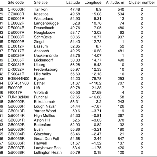
Table 1.List of the sites used for analysis. Negative values in latitude denote to the Southern

Hemisphere, negative values in longitude denote to western longitudes.

Site code Site title Latitude Longitude Altitude, m Cluster number

1 ALG447N00 Algoma 47.03 −84.38 411 1

2 BMW432N40 Tudor Hill 32.37 −64.65 30 1

3 CHA446N00 Chalk River 46.07 −77.4 184 1

4 ELA449N00 Experimental Lakes Area 49.67 −93.72 369 1

5 FI0022R Oulanka 66.32 29.4 310 1

6 GB0015R Strath Vaich Dam 57.73 −4.77 270 1

7 IE0031R Mace Head 53.17 −9.5 15 1

8 MCM777S40 McMurdo/Arrival Height −77.8 166.77 50 1

9 MNM224N00 Minamitorishima 24.3 153.97 8 1

10 NO0015R Tustervatn 65.83 13.92 439 1

11 NO0039R K ˚arvatn 62.78 8.88 210 1

12 NO0042G Spitsbergen, Zeppelinfjell 78.9 11.88 474 1

13 NO0048R Voss 60.6 6.53 500 1

14 RYO239N00 Ryori 39.03 141.82 260 1

15 SE0013R Esrange 67.88 21.07 475 1

16 SPO789S40 South Pole −89.98 −24.8 2810 1

17 AT0002R Illmitz 47.77 16.77 117 2

18 AT0030R Pillersdorf bei Retz 48.72 15.94 315 2

19 AT0033R Stolzalpe bei Murau 47.13 14.2 1302 2

20 AT0042R Heidenreichstein 48.88 15.05 570 2 21 AT0045R Dunkelsteinerwald 48.37 15.55 320 2 22 AT0046R G ¨anserndorf 48.33 16.73 161 2 23 AT0047R Stixneusiedl 48.05 16.68 240 2 24 BE0001R Offagne 49.88 5.2 430 2 25 BE0032R Eupen 50.63 6 295 2 26 BE0035R Vezin 50.5 4.99 160 2 27 CH0002R Payerne 46.82 6.95 510 2

(24)

ACPD

7, 12541–12572, 2007

Full Screen / Esc

Table 1.Continued.

28 CH0003R T ¨anikon 47.48 8.9 540 2

29 CZ0003R Kosetice 49.58 15.08 534 2

30 DE0001R Westerland 54.93 8.31 12 2

31 DE0002R Langenbr ¨ugge 52.8 10.76 74 2

32 DE0004R Deuselbach 49.76 7.05 480 2 33 DE0007R Neuglobsow 53.17 13.03 62 2 34 DE0008R Schm ¨ucke 50.65 10.77 937 2 35 DE0009R Zingst 54.43 12.73 1 2 36 DE0012R Bassum 52.85 8.7 52 2 37 DE0017R Ansbach 49.25 10.58 481 2

38 DE0026R Ueckerm ¨unde 53.75 14.07 1 2

39 DE0035R L ¨uckendorf 50.83 14.77 490 2 40 DK0031R Ulborg 56.28 8.43 10 2 41 DK0032R Frederiksborg 55.97 12.33 10 2 42 DK0041R Lille Valby 55.69 12.13 10 2 43 EGB444N00 Egbert 44.23 −79.78 253 2 44 EST451N00 Esther 51.67 −110.2 707 2 45 FI0009R Ut ¨o 59.78 21.38 7 2 46 FI0017R Virolahti 60.53 27.69 4 2 47 FUN132N00 Funchal 32.65 −16.88 58 2 48 GB0002R Eskdalemuir 55.31 −3.2 243 2 49 GB0006R Lough Navar 54.44 −7.87 126 2 50 GB0013R Yarner Wood 50.6 −3.71 119 2 51 GB0014R High Muffles 54.33 −0.81 267 2 52 GB0031R Aston Hill 52.5 −3.03 370 2 53 GB0032R Bottesford 52.93 −0.82 32 2 54 GB0033R Bush 55.86 −3.21 180 2 55 GB0034R Glazebury 53.46 −2.47 21 2

56 GB0035R Great Dun Fell 54.68 −2.44 847 2

57 GB0036R Harwell 51.57 −1.32 137 2

58 GB0037R Ladybower Res. 53.4 −1.75 420 2

(25)

ACPD

7, 12541–12572, 2007

Full Screen / Esc

EGU

60 GB0039R Sibton 52.29 1.46 46 2 61 GB0043R Narberth 51.23 −4.7 160 2 62 IT0004R Ispra 45.8 8.63 209 2 63 KEJ444N00 Kejimkujik 44.43 −65.2 127 2 64 KPS646N00 K-puszta 46.97 19.55 125 2 65 LT0015R Preila 55.35 21.07 5 2 66 LV0010R Rucava 56.22 21.22 5 2 67 NL0009R Kollumerwaard 53.33 6.28 1 2 68 NL0010R Vredepeel 51.54 5.85 28 2 69 NO0001R Birkenes 58.38 8.25 190 2 70 NO0041R Osen 61.25 11.78 440 2 71 NO0043R Prestebakke 59 11.53 160 2 72 NO0045R Jeløya 59.43 10.6 5 2 73 PL0002R Jarczew 51.82 21.98 180 2 74 PL0004R Leba 54.75 17.53 2 2 75 PL0005R Diabla Gora 54.15 22.07 157 2 76 PT0004R Monte Velho 38.08 −8.8 43 2 77 SAT448N00 Saturna 48.78 −123.13 178 2 78 SE0002R R ¨orvik 57.42 11.93 10 2 79 SE0011R Vavihill 56.02 13.15 175 2 80 SE0012R Aspvreten 58.8 17.38 20 2 81 SE0032R Norra-Kvill 57.82 15.57 261 2 82 SE0035R Vindeln 64.25 19.77 225 2

83 SK0004R Star ´a Lesn ´a 49.15 20.28 808 2

84 SK0006R Starina 49.05 22.27 345 2

85 SK0007R Topolniky 47.96 17.86 113 2

86 TKB236N30 Tsukuba 36.05 140.13 25 2

87 USI354S0 Ushuaia −54.85 −68.32 18 2

88 BAR541S00 Baring Head −41.42 174.87 85 3

89 BRW471N40 Barrow 71.32 −156.6 8 3

90 NMY770S00 Neumayer −70.65 −8.25 42 3

(26)

ACPD

7, 12541–12572, 2007

Full Screen / Esc

92 AT0034G Sonnblick 47.05 12.96 3106 4

93 AT0037R Zillertaler Alpen 47.14 11.87 1970 4

94 AT0038R Gerlitzen 46.69 13.92 1895 4 95 JFJ646N00 Jungfraujoch 46.55 7.98 3578 4 96 NWR440N40 Niwot Ridge 40.03 −105.53 3022 4 97 SI0032R Krvavec 46.3 14.54 1740 4 98 AT0004R St.Koloman 47.65 13.2 851 5 99 AT0032R Sulzberg 47.53 9.93 1020 5 100 AT0040R Masenberg 47.35 15.88 1170 5 101 AT0041R Haunsberg 47.97 13.02 730 5 102 AT0043R Forsthof 48.11 15.92 581 5

103 AT0044R Graz Platte 47.11 15.47 651 5

104 CH0004R Chaumont 47.05 6.98 1130 5 105 CH0005R Rigi 47.07 8.47 1030 5 106 CZ0001R Svratouch 49.73 16.03 737 5 107 DE0003R Schauinsland 47.91 7.91 1205 5 108 DE0005R Brotjacklriegel 48.82 13.22 1016 5 109 HPB647N00 Hohenpeissenberg 47.8 11.02 985 5

110 LIS638N00 Lisboa/Gago Coutinho 38.77 −9.13 105 5

111 PL0003R Sniezka 50.73 15.73 1603 5

112 SI0031R Zarodnje 46.43 15 770 5

113 SI0033R Kovk 46.13 15.11 600 5

(27)

ACPD

7, 12541–12572, 2007

Full Screen / Esc

EGU

Table 2. Statistical information on the observational and model clusters. One-σ shows a

stan-dard deviations range in the estimate of the clusters centers (Figs. 1, 4) as an average of N cluster members. Each range is representative for 288 values.

Observational cluster Number of sites included One-σ of OC centers: range, (average), nmol/mol Identified type (OC) Mostly over-lapping model cluster Number of the grid cells included One-σ of MC centers: range, (average), nmol/mol Comment on MC #1 16 2.5–7.9 (4.6) clean – ru-ral #2 43 3.2–11.8 (6.8) #2 71 3.7–9.4 (5.4) semi-polluted non-elevated #3 4 2.3–5.7 (4.1) polar – re-mote #1 6 1.7–5.8 (3.0) southern-hemispheric

#4 6 1.0–6.2 (2.6) elevated Included in MC #2 and #4

#5 17 1.8–5.2 (3.4)

semi-polluted semi-elevated

#4 21 1.8–12.5 (6.1)

Included in OC #1 and #2 #3 2 0–6.1 (2.0) island

(28)

ACPD

7, 12541–12572, 2007

Full Screen / Esc

Printer-friendly Version Interactive Discussion (a) 0 2 4 6 8 10 12 14 16 18 20 22 2 4 6 8 10 12 cluster 1 12,0 14,5 17,0 19,5 22,0 24,5 27,0 29,5 32,0 34,5 37,0 39,5 42,0 44,5 47,0 49,5 52,0 54,5 55,0 local time, h month (b) 0 2 4 6 8 10 12 14 16 18 20 22 2 4 6 8 10 12 cluster 2 12,0 14,5 17,0 19,5 22,0 24,5 27,0 29,5 32,0 34,5 37,0 39,5 42,0 44,5 47,0 49,5 52,0 54,5 55,0 local time, h month (c) 0 2 4 6 8 10 12 14 16 18 20 22 2 4 6 8 10 12 cluster 3 12,0 14,5 17,0 19,5 22,0 24,5 27,0 29,5 32,0 34,5 37,0 39,5 42,0 44,5 47,0 49,5 52,0 54,5 55,0 local time, h month (d) 0 2 4 6 8 10 12 14 16 18 20 22 2 4 6 8 10 12 cluster 4 12,0 14,5 17,0 19,5 22,0 24,5 27,0 29,5 32,0 34,5 37,0 39,5 42,0 44,5 47,0 49,5 52,0 54,5 57,0 59,5 60,0 local time, h month (e) 0 2 4 6 8 10 12 14 16 18 20 22 2 4 6 8 10 12 cluster 5 12,0 14,5 17,0 19,5 22,0 24,5 27,0 29,5 32,0 34,5 37,0 39,5 42,0 44,5 47,0 49,5 52,0 54,5 55,0 local time, h month

Fig. 1. Seasonal – diurnal cycles for the 5 clusters representing 114 observed time series as

described in the text. The color scale shows the mixing ratio in nmol/mol. The following clusters are identified: (a) clean/rural; (b) semi-polluted non-elevated; (c) polar/remote; (d) elevated and

(e)semi-polluted semi-elevated. The cluster memberships are listed in Table 1. For cluster 4

(29)

ACPD

7, 12541–12572, 2007

Full Screen / Esc

Printer-friendly Version Interactive Discussion EGU 0 2 4 6 8 10 12 14 10 15 20 25 30 35 40 45 50 55 60 O3 , nmol/mol month month month month month O3 , nmol/mol month

cluster 1 cluster 2 cluster 3 cluster 4 cluster 5

0 2 4 6 8 10 12 14 10 15 20 25 30 35 40 45 50 55 60 4 h local time 0 h local time 0 2 4 6 8 10 12 14 10 15 20 25 30 35 40 45 50 55 60 16 h local time 12 h local time 8 h local time 0 2 4 6 8 10 12 14 10 15 20 25 30 35 40 45 50 55 60 0 2 4 6 8 10 12 14 10 15 20 25 30 35 40 45 50 55 60 20 h local time 0 2 4 6 8 10 12 14 10 15 20 25 30 35 40 45 50 55 60

Fig. 2. _{Seasonal cycle of the surface ozone mixing ratio in different measurement clusters for}

selected time of the day (the data obtained as a subset of the full picture presented in Fig. 1). The mixing ratio scale is the same in all graphs to show the levels differences between the clusters and to reflect their diurnal changes.

(30)

ACPD

7, 12541–12572, 2007

Full Screen / Esc

Printer-friendly Version Interactive Discussion (a) -180 -150 -120 -90 -60 -30 0 30 60 90 120 150 180 -90 -60 -30 0 30 60 90 MEASUREMENTS cluster 1 cluster 2 cluster 3 cluster 4 cluster 5 La ti tude ( N ) Longitude (E) (b) -180 -150 -120 -90 -60 -30 0 30 60 90 120 150 180 -90 -60 -30 0 30 60 90 MODEL cluster 1 cluster 2 cluster 3 cluster 4 La ti tude ( N ) Longitude (E) (c) -20 -10 0 10 20 30 30 40 50 60 70 80 MEASUREMENTS cluster 1 cluster 2 cluster 3 cluster 4 cluster 5 Lat it ude ( N ) Longitude (E) _(d) -20 -10 0 10 20 30 30 40 50 60 70 80 MODEL cluster 1 cluster 2 cluster 3 cluster 4 Lat it ude ( N ) Longitude (E)

Fig. 3. _{Spatial distribution of the sites of different clusters (a). The clusters obtained for the}

ECHAM5/MESSy1 output are also presented on the maps (b). The model points are placed to the sites closest to the center of the grid. In the lower panel (c–d) Europe is shown in more details.

(31)

ACPD

7, 12541–12572, 2007

Full Screen / Esc

Printer-friendly Version Interactive Discussion EGU (a) 0 2 4 6 8 10 12 14 16 18 20 22 1 2 3 4 5 6 7 8 9 10 11 12 model cluster 1 12,0 14,5 17,0 19,5 22,0 24,5 27,0 29,5 32,0 34,5 37,0 39,5 42,0 44,5 47,0 49,5 52,0 54,5 55,0 local time, h month (b) 0 2 4 6 8 10 12 14 16 18 20 22 1 2 3 4 5 6 7 8 9 10 11 12 model cluster 2 12,0 14,5 17,0 19,5 22,0 24,5 27,0 29,5 32,0 34,5 37,0 39,5 42,0 44,5 47,0 49,5 52,0 54,5 55,0 local time, h month (c) 0 2 4 6 8 10 12 14 16 18 20 22 1 2 3 4 5 6 7 8 9 10 11 12 model cluster 3 12,0 14,5 17,0 19,5 22,0 24,5 27,0 29,5 32,0 34,5 37,0 39,5 42,0 44,5 47,0 49,5 52,0 54,5 55,0 local time, h month (d) 0 2 4 6 8 10 12 14 16 18 20 22 1 2 3 4 5 6 7 8 9 10 11 12 model cluster 4 10,0 12,5 15,0 17,5 20,0 22,5 25,0 27,5 30,0 32,5 35,0 37,5 40,0 42,5 45,0 47,5 50,0 52,5 55,0 57,5 60,0 62,5 65,0 local time, h month (e) 0 2 4 6 8 10 12 10 15 20 25 30 35 40 45 50 55 60 65 O3 , nmol/mol month 0 h local time 4 h local time 8 h local time 12 h local time 16 h local time 20 h local time

Fig. 4.Seasonal-diurnal ozone cycles for the 4 clusters of the ECHAM5/MESSy1 model output

sub-sampled at the measurement sites locations. Colors and units are as in Fig. 1. The scale for cluster 4 is extended to lower and higher values in comparison with the other clusters. Panels (a–d) present the cluster averages, panel (e) shows seasonal cycles for the model cluster 4 at the selected hours as a subset of the panel (d).