Enhancing the reusability and interoperability of artificial neural networks with DEVS modeling and simulation

HAL Id: hal-01719242

https://hal.uca.fr/hal-01719242

Submitted on 21 Oct 2020

HAL is a multi-disciplinary open access archive for the deposit and dissemination of sci-entific research documents, whether they are pub-lished or not. The documents may come from teaching and research institutions in France or

L’archive ouverte pluridisciplinaire HAL, est destinée au dépôt et à la diffusion de documents scientifiques de niveau recherche, publiés ou non, émanant des établissements d’enseignement et de recherche français ou étrangers, des laboratoires

Enhancing the reusability and interoperability of

artificial neural networks with DEVS modeling and

simulation

David Ifeoluwa Adelani, Mamadou Kaba Traoré

To cite this version:

David Ifeoluwa Adelani, Mamadou Kaba Traoré. Enhancing the reusability and interoperability of artificial neural networks with DEVS modeling and simulation. International Journal of Model-ing, Simulation, and Scientific ComputModel-ing, World Scientific PublishModel-ing, 2016, 07 (02), pp.1650005. �10.1142/S1793962316500057�. �hal-01719242�

1

ENHANCING THE REUSABILITY AND INTEROPERABILITY

OF ARTIFICIAL NEURAL NETWORKS WITH DEVS

MODELING AND SIMULATION

David Ifeoluwa Adelani Department of Computer Science African University of Science and Technology,

Abuja, Nigeria Email: davlanade@gmail.com

Mamadou Kaba Traore LIMOS, CNRS UMR 6158

Université Blaise Pascal, Clermont-Ferrand 2 Campus des Cezeaux, 63173 Aubiere,

E-mail: traore@isima.fr

ABSTRACT

Artificial Neural Networks (ANNs), a branch of Artificial Intelligence has become a very interesting domain since the eighties when back-propagation learning algorithm for multi-layer feed-forward architecture was introduced to solve non-linear problems. It is used extensively to solve complex non-algorithmic problems such as prediction, pattern recognition, and clustering. However, in the context of a holistic study, there may be a need to integrate ANN with other models developed in various paradigms to solve a problem. In this paper, we suggest Discrete Event System Specification (DEVS) be used as a Model of Computation (MoC) to make ANN models interoperable with other models (since all discrete event models can be expressed in DEVS, and continuous models can be approximated by DEVS). By combining ANN and DEVS, we can model the complex configuration of ANNs and express its internal workings. Therefore, we are extending the DEVS-Based ANN proposed by Toma et al [1] for comparing multiple configuration parameters and learning algorithms and also to do prediction. The DEVS models are described using the High Level Language for System Specification (HiLLS)[2], a graphical modeling language for clarity. The developed platform is a tool to transform ANN models into DEVS computational models, making them more reusable and more interoperable in the context of larger multi-perspective modeling and simulation.

Keywords: Artificial Neural Networks, DEVS, Z-Schema, reusability, interoperability, HiLLS,

Learning Algorithm, Modeling and Simulation.

1. INTRODUCTION

Modeling and Simulation (M&S), the third pillar of science is a paradigm that provides a way of obtaining the behavior of the representation of an object in real life without doing physical experiments. Modeling complex systems requires a robust formalism. The Discrete Event System Specification (DEVS) formalism [3] which was introduced in the early 70’s is a theoretically well-defined formalism for modeling discrete event systems in a hierarchical and modular manner. It allows the behavior modeling of complex systems.

Artificial Neural Networks (ANN) is a branch of artificial intelligence that became popular in the eighties when the back-propagation algorithm [4] for multilayer feed-forward architectures was introduced. Moreover, it is widely known that classical neural networks, even with one hidden

layer, are universal function approximators [5]. ANNs became widely applicable for real applications when it had the capabilities to solve non-linear problems. It is used for modeling of complex optimization problems such as classification, prediction and pattern recognition.

In the context of a holistic approach in modeling a complex system, there may be need to integrate ANN with other models developed in various paradigms (like continuous systems and discrete systems). Reusability and Interoperability are two important concepts in holistic modeling approach. The reuse of simulation models should reduce the time and cost for model development. Hence, a trained ANN can be reused severally to predict new results required by other models when provided with new set of inputs. On the other hand, interoperability is the ability of two or more systems to exchange information and to use the information that has been exchanged [6]. Generally, the communicating systems may be of different paradigms; for interoperability to be achieved, some degree of compatibility must exists among all elements that must cooperate in some purpose [7]. Therefore, a robust modeling formalism is needed to integrate ANN models with models of different paradigms to achieve interoperability.

DEVS formalism has been shown to be robust for modeling hybrid systems [8] since all discrete event models can be expressed in DEVS and continuous models can be approximated [9] by DEVS. The benefit of using ANNs is its capability of modeling complex non-linear systems using adaptive learning mechanism to derive meaning from complicated or imprecise data with a high degree of accuracy. By modeling ANNs in DEVS, we can have a hybrid model composed of ANN models, discrete models and continuous models. Without this, it will not be convenient to efficiently interoperate this dynamic model with other models. Combining DEVS and ANN is possible because ANNs are by default using discrete events i.e., the network is always waiting to an input event to generate an output one. Toma et al [1] proposed an approach for describing the structure of ANN with DEVS known as DEVS-Based ANN. This approach was said to be able to facilitate the network configuration that depends a lot on ANN. Our focus is to present DEVS as a Model of Computation (MoC) to make ANN models interoperable with other models.

We propose to extend the work in [1] for comparing multiple configuration parameters and learning algorithms. The approach makes it flexible to do prediction after training by disconnecting the DEVS models associated with learning. This will help users and developers test and compare different algorithm implementations and parameter configurations. HiLLS, a graphical modeling language will be used to describe the approach for a clear understanding. Also, we will describe the benefits (reusability and interoperability) of transforming ANN models into DEVS computational models in the context of larger multi-perspective modeling and simulation.

This paper is structured as follows. In section 2, we describe DEVS and ANN learning algorithms and configuration parameters. In section 3, we review some related works. In section 4, we present the extended DEVS-Based ANN approach. In section 5, we describe the benefits of DEVS-Based ANN and section 6 concludes the paper.

3 2. BACKGROUND

2.1. Artificial Neural Networks (ANN)

ANN models the way biological neurons process information to solve complex non-algorithmic problems like recognizing patterns, classifying into groups, series prediction. An artificial neuron is composed of set of inputs, connection weights, activation function and outputs. ANN has been a subject of active research from as early as 1943 when McCulloch and Pitt[10] designed the first neural network. Donald Hebb [11] in 1949 designed the first learning rule for ANN since they learn by example to solve problems. In the 1950 and 60’s, many researchers (Block, Minsky, Papert and Frank Rosenblatt [12]) introduced and developed a large class of artificial neural networks called perceptrons that proved to converge to the correct weights. However, the perceptron could not learn non-linear separable functions, this cause a decline in research in neural networks until back propagation algorithm [13] was discovered to solve the problem.

2.1.1. Architecture of ANN

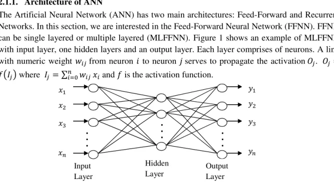
The Artificial Neural Network (ANN) has two main architectures: Feed-Forward and Recurrent Networks. In this section, we are interested in the Feed-Forward Neural Network (FFNN). FFNN can be single layered or multiple layered (MLFFNN). Figure 1 shows an example of MLFFNN with input layer, one hidden layers and an output layer. Each layer comprises of neurons. A link with numeric weight from neuron to neuron serves to propagate the activation . =

where = ∑ and is the activation function.

The basic operation of an artificial neuron involves summing its weighted input signal an activation function to produce a calculated output. The input layer makes use of identity function ( ( = . For hidden and output layers, a non-linear activation function (see figure 2) is used. The activation function is expected to be continuous, differentiable and monotonically non-decreasing. For computational efficiency, its derivative be easy to compute [14].

.

.

.

.

.

.

.

.

.

Figure 1: A Multilayer Feed-Forward Neural Architecture

Figure 2: Activation Functions

2.1.2. Learning Algorithm

The power of ANN comes from the learning process. It needs to be trained to map an input vector to the targeted output. Depending on the learning algorithm used to train them, they can learn either very fast or very slow. There are two major types of learning algorithms – supervised and unsupervised learning. In this paper, we are interested in supervised learning – neural networks learn from a set of sample data. Typically, supervised learning uses gradient descent for the minimization of errors between the desired output and calculated output.

The Back Propagation (BP) algorithm is the most popular learning rule for supervised learning. It uses a gradient-based technique to minimize the error function equivalent to the Mean Square Error (MSE) between the desired and actual network outputs. The BP algorithm propagates backward the error between the desired signal and the network output through the network. The new error is used to update the weights for a feed-forward process. The steps of BP are:

1. Configuration and Input of Parameters: set of training samples each with input and output vectors (x, t), a multilayer network with L layers, learning rate ( ), minimum error, epoch.

2. Weight initialization: set a small random number for for layer to layer connection.

While termination condition is not met do For each sample (x, t) in the training set do

3. Feed-Forward Calculation: The input layer activation is identity ( = ∀

for l=2 to L do

= ∑

=

4. Error Correction (or Learning)

The error for the output layer is ! = "_{( − $ (2.1)}

for l=L-1 to 1 do

! = "_{( (∑ ! (2.2)} Δ = _&(&'

)* = ! (2.3)

($ + 1 = ($ + Δ (2.4)

One of the drawbacks of using the error gradient function to calculate the error is being trapped in a local minima and never getting the global minima. To solve this problem, a momentum term was introduced in the BP algorithm [4] by Rumelhart. The weight change is in a direction that is a combination of the current gradient and the previous gradient. Equation 2.3 becomes Δ ($ = _&(&'

)* + - Δ ($ − 1

We considered some other algorithms that tries to optimize equation 2.3 : Silva & Almeida [15] , Delta-Bar-Delta [16], QuickProp [17] and Resilient Propagation [18] (RPROP). Schiffmann et al [18] gives a very good description of these algorithms

5 2.2. Discrete Event System Specification (DEVS)

The Discrete event system specification (DEVS) is a formalism introduced by Zeigler in 1976 to describe discrete event system in a hierarchical and modular manner. It is theoretically well-defined system formalism [20]. The DEVS models are seen as black boxes with input and output ports used to describe system structure as well as system behavior. As a result, DEVS offers a platform for modeling and simulation (M&S) of complex systems in different domains.

2.2.1. Atomic Model

An atomic model is defined as a 7-tuple ./ =< 1, 3, 4, ! 5, !675, 8, $9 > where 1 = set of input events

3 = set of output events 4 is the set of state variables

! 5: 4 → 4 is the internal transition function $9: 4 → ℝ>_{,>? is the time advance function}

!675: @ × 1 → 4 is the external transition function.

where @ = B( , | ∈ 4, ∈ E0, $9( GHis the set of total states and e is the time elapsed since the last transition

8: 4 → 3 is the output function

A DEVS model is always in a state ∈ 4 at a given time. The model can transit from one state to another using transition functions ! ₅ and !₆₇₅. In the absence of external events, it remains in the state for a lifetime of $9( . When ta(s) is reached, the model outputs value ∈ 3 through its port using the output function 8( , then it changes to a new state defined by ! ₅( . In the case of an external events triggered by external inputs, the external transition function determines the new state given by !₆₇₅( , , , where is the current state, is the time elapsed since the last transition, and ∈ 1 is the external event received.

22.2.2. Coupled Model

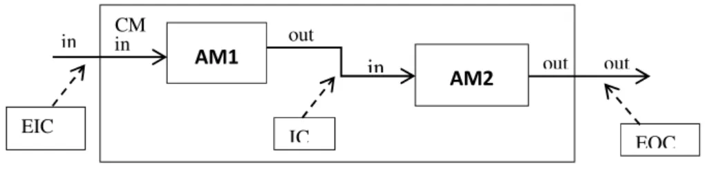
A DEVS coupled model is composed of several atomic or coupled sub-models with three possible kinds of coupling: Internal coupling (IC), input coupling (EIC) and external-output coupling (EOC) as shown in the diagram below.

There are many implementation of DEVS formalism [21]. However, for this paper, we made use of SimStudio Simulation Package (a component of SimStudio[21]) – an Object-Oriented implementation of simulation algorithm for C-DEVS and P-DEVS written in Java.

Figure 3: Example of a Coupled Model

CM _out AM1 AM2 out in in out in IC _EOC EIC

2.3. High Level Language for System Specification (HiLLS)

HiLLS evolved from the DEVS-Driven Modeling Language (DDML)[22], a graphical modeling language built on DEVS to facilitate the use of the latter by domain experts via user-friendly graphical concrete syntax to describe system models. The goal of HiLLS is to be able to create multi-semantic models that can be used for simulation, formal analysis and enactment. HiLLS' syntax combines system-theoretic and Software Engineering concepts adopted from the DEVS and Object-Z [23] (to express functional and behavioral properties) respectively.

The concrete notations to express HiLLS' concepts are described in Figure 4(a-h). HClass (a) and HSystem (b) are similar to the UML class symbol but with Object-Z notations for state schema and axiomatic schema. It uses DDML borrowed concepts for the state configurations (Fig. c-e) and state transitions (g-h). For more details, see [2]. The choice of HiLLS is its ability to model dynamic structure systems (DSS) and ANN is a good example. Moreover, HiLLS was shown to be able to model Dynamic Structure DEVS (DSDEVS) using its rich concrete syntax [2]. However, HiLLS does not support input and output interfaces structural changes. This is not a challenge since the DEVS-Based ANN parameters are defined before simulation starts.

7 3. RELATED WORKS

Neural networks have been used extensively to determine the behavior of discrete event systems because it can learn from empirical data but little research is focused on using discrete event modeling to specify the structure and components of a neural network. Sung Hoon Jung and Tag Gon Kim in [24] made use of neural network as an interface between continuous system and discrete event system. The trained neural network provided the state transition rules (and can also predict new rules) for the DEVS model abstracted from the continuous system. Si Jong Choi and Tag Gon Kim [25] were able to extract a DEVS model after the behavior learning of a Compound Recurrent ANN (CRNN). They showed that a trained CRNN is behaviorally equivalent to FM-DEVS model. Jean-Baptiste Filipi et al [26] proposed Neuro-DEVS by extending the DEVS atomic model with functions like activation function, learning function and connection links. Neuro-DEVS hybrid system offers comparative, concurrent and adaptive simulation since DEVS and ANN are in the same box although of different paradigms.

In modeling the complex structures of ANN, S. Vahie [27] made use of discrete event modeling formalism to model the neurobiological components(dendrite, cell body and axon) of the neural network in order to increase the computational power, adaptability and dynamic response of ANNs. He proposed a DEVS model called Dynamic Neuronal Ensembles (DNE). The DNE is a coupled model of components that are themselves coupled models called dynamic neurons (DN). However, the huge number of messages transferred among DNE will cause a slow simulation.

S. Toma et al [1] described the structure of ANN with DEVS atomic and coupled models. Each layer of ANN is an atomic model which was categorized into non-calculation (input layer) and calculation layer (hidden and output layer). Two additional atomic DEVS models were added for the learning phase: Error-Generator and Delta-Weight Model. Their approach offers a good visual representation of ANN, easy network configuration and also the clear separation of the feed-forward calculation models and learning models which makes it possible to do prediction when the Delta-Weight Models are disconnected. However, prediction was not implemented. The platform is known as DEVS-Based ANN and Momentum BP was the only learning algorithm used.

In this paper, we present DEVS as Model of Computation (MoC) for ANNs to make them more reusable and interoperable. From the works of Tag Gon Kim [23] [24], the ability of ANNs to derive meaning from imprecise data using adaptive learning mechanism was useful for providing transition rules for DEVS. In holistic approach, if the ANNs were modeled with DEVS, the trained ANN sub-model will be more reusable since new predicted outputs generated can serve as inputs for other sub-model(s). Also, having various models from different paradigms modeled in a single robust modeling paradigm enhances efficiency and interoperability among sub-models.

We validated and extended the DEVS-Based ANN by incorporating 6 learning algorithms and 4 activation functions described in section 2. This will help modelers to test, compare and choose

the best algorithm and parameter configuration suitable for solving a non-linear problem. Also, we have added prediction feature to the DEVS-Based ANN platform. For a clear understanding of the DEVS Model, we will make uses of HiLLS, a graphical modeling language to describe the models taking into consideration the parameter configurations such as number of hidden layers, output neurons for each layer and stopping condition (minimum error or maximum number of iterations). This allows for more expressible models of DEVS-Based ANN.

4. DEVS-Based ANN APPROACH

4.1. DEVS-Based ANN Modeling

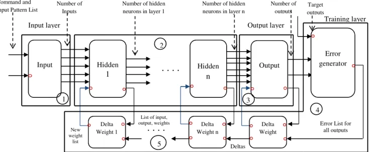
In this section, we will describe the four atomic models in the DEVS-Based ANN [28] representing the ANN layers and the separate learning models. The first model is the non-calculation (or input) layer that forwards inputs to the first non-calculation (hidden) layer. The calculation layer model describes the structure of the hidden and output layers. Error-Generator and Delta-Weight are the two models that are used by the ANN learning phase. After the neural network has been trained, one can do prediction by simply removing the learning models.

All the ports with circle are ports used only in training phase. As shown in the Figure 5, the connections between the training layer and the calculation models are basically for learning purposes. The Input atomic model forwards data to the hidden layer (shown in step 1 in the figure), and then each hidden layer (including the Output layer) computes the weighted sum and activation functions. In steps 2 and 3, each hidden or output layer sends output data to the next layer and learning data (inputs, outputs and weights) to the delta-weights. As soon as the output layer sends its output (ANN calculated outputs) to the error-generator model, it sends error (difference between the target output and calculated output) to the Delta-Weight models (step 4).

Figure 5: DEVS-Based Neural Networks Architecture

Training layer

Input layer Output layer

Command and Input Pattern List

Number of Inputs Number of hidden neurons in layer 1 Number of hidden neurons in layer n Number of outputs Target outputs Input Hidden 1 Hidden n Output

. . . .

. . . .

Error List for all outputs Deltas

4 4

9

The Delta-Weight model calculates the new error (delta) from the learning data and the weight change from any of the gradient descent algorithms specified. After that, the delta-weight model will back-propagate error to another delta-weight model if it exist and weight list will be sent to the corresponding calculation layer (step 5). The entire cycle explained above is considered as one learning iteration (or epoch) that is repeated (steps from 1 to 5) depending on the stopping condition.

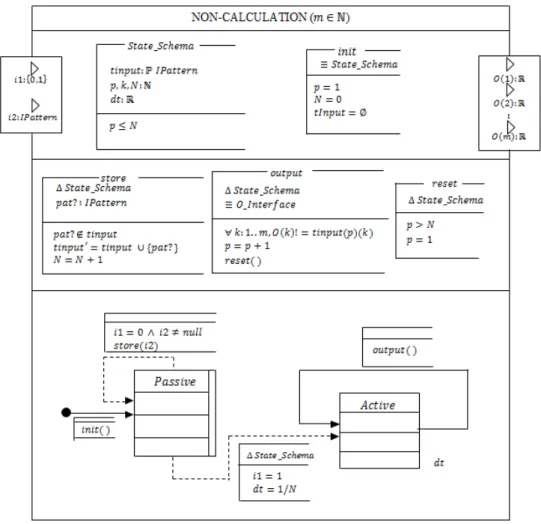
4.1.1. Non-Calculation Layer Atomic Model (NC)

IPattern: is a list of inputs or outputs in a single pattern (usually many patterns are used for

training a neural network). IJKLMI: is the list of all training patterns. N O$ 1 is added to signal to the NC model that all training patterns have been sent. is the number of inputs

Figure 6: Non-Calculation Model

The DEVS atomic model is in a passive state with $9 = +∞. When an event is received from port 2 (input pattern), the input pattern is stored and a counter Q is incremented. However, on receiving a ‘1’ message from the first port, the model computes $ = 1/Q, and transits to an

active state. The model remains active with a life time of 1/Q, it forwards each value in the input pattern list through different output ports to the calculation layer.

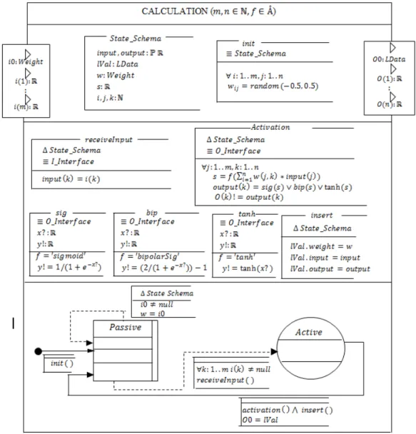
4.1.2. Calculation Layer Model

STUVWI: is a data type expressed as to shows connection between i input and j output. XYZIZ: is expressed as a record that has weights, input and output. The values are needed by the DELTA-WEIGHT model. [ is the number of input neurons and K is the number of output neurons.

Figure 7: Calculation Model

The calculation layer model represents any hidden or output layer, as both layers have the same behavior. The calculation layer has two special ports reserved for learning: one among the input ports (port a) and the other among the output ports (port b) as shown in Figure 7.

11

The model is in a passive state with $9 = +∞. When messages are received through the input ports (except port a), it transits to an active state with $9 = 0. Immediately, it computes the calculated outputs through the activation function; after which it sends the calculated outputs through its output ports and the learning data through port b before returning to passive state. If message is received from port a, the weights of the layer are updated.

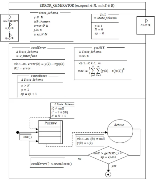
4.1.3. Error Generator Model

[ is the number of calculated outputs. [UK\ is the minimum error.

Figure 8: Error Generator Model

The model receives calculated output from the last calculation layer (output layer) and also target outputs. It compares the two outputs by computing the difference known as error. In an ideal situation, the error between the target output and calculated output should be zero. Unfortunately,

there is always a percentage error. The error list is forwarded to the delta-weight atomic model of the corresponding output layer to re-calibrate the network for better performance.

In figure 8, the model has one special input port for target output list (port a). The model is in a passive state with $9 = +∞. When a message is received from port a, the model stores the output pattern and increment a variable (Q = Q + 1 ; but it remains in the passive state. However, if there are inputs from other ports, the model transit to an active state with $9 = 0 where the error ]_^ is computed.

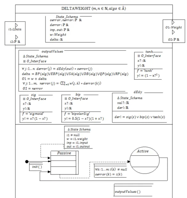
4.1.4. Delta-Weight Model

Figure 9: Delta-Weight Model

The Delta-Weight model has two input ports and two output ports. It receives learning data from the calculation layer through the first input port. The learning data consist of the input, output

13

and weight list of the corresponding calculation layer. On the other hand, the second port receives the error list from another weight model or error generator (for the last delta-weight). The Delta-Weight model has two states (passive and active).

In figure 9, the model is in a passive state with $9 = +∞. When it receives a message from the first port, it stores the learning data required for weight update and remains in the passive state. On receiving a message from the second port, it transits to active state with $9 = 0; then, it computes the new error and the new weights. The new error is sent to another delta-weight model if available while the new weights are sent to the corresponding calculation model.

4.2. Implementation and Results

The DEVS model described in section 4.1 is implemented with the SimStudio DEVS framework in JAVA programming language. It is a coupled model with 6 atomic models namely:

InputGenerator, TargetGenerator, InputLayer, CalculationLayer, ErrorGenerator and

DeltaWeight. For each run, we need to specify the learning rate, momentum, activation function,

learning algorithm, training input pattern list, training target pattern list, number of hidden

neurons for each hidden layer and the minimum error.

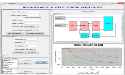
A Graphical user friendly platform has been developed to facilitate the modeling and simulation approach of the DEVS-Based ANN system. When the configuration parameters are set, weights are randomly generated into initWeights.txt before training. The platform has the ability to build a neural network model with several activation functions and learning algorithms for a multi-layer neural network. It can also do prediction for a trained network using an updated weight list stored in a text file. The platform has 3 sections: Parameter configuration and execution, DEVS model design and graph results. Figure 10 shows an example of algorithm comparison in XOR.

Figure 10: Algorithm Comparison for XOR function

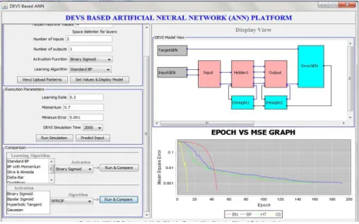
Figure 11 shows an XOR function result with multiple activation functions (Binary sigmoid, Bipolar sigmoid, Hyperbolic tangent and Gaussian) and Resilient propagation algorithm. The

learning rate of 0.3 and momentum of 0.7 was used. Also, a minimum error of 0.001 was used to compare the activation functions.

Figure 11: Comparison of Activation Functions in XOR

A practical example is gotten from UCI Machine Learning Repository [29] to classify wine samples into 3 different types represented as 1 0 0, 0 1 0, and 0 0 1 respectively. The data set consists of 178 input patterns and each one is described with 13 characteristics However, we will be using 27 input patterns for the training of the neural networks and 3 for test inputs. (see figure 12 and 13)

15 Figure 13: Test Input for Wine Samples

5. BENEFITS OF DEVS-BASED ANN IN HOLISTIC MODELING APPROACH

For the analysis and design of such complex systems, it is convenient to transform all models to the same modeling formalism as in Figure 13. We suggested DEVS because all discrete event models can be expressed in DEVS, and continuous models can be approximated [30] by DEVS.

Non-linear dynamical systems (e.g. ANN) DEVS MODEL M1 Discrete Event Systems (e.g DEVS,

State charts, Petri-nets, cellular Automata, FSA) Continuous systems (e.g ODE, PDE) DEVS MODEL M3 DEVS MODEL M2 DEVS MODEL M5 DEVS MODEL M4 Stochastic systems (e.g markov Chains) Transformed by DEVS-Based ANN

DES can be easily

transformed Transformed by

quantization (GDEVS)

Transformed by STDEVS

Figure 13: Holistic Modeling Approach

Coupled DEVS Model

Also, DEVS has been shown to model stochastic systems [31] using stochastic DEVS (STDEVS). The new platform DEV-Based ANN (described in section 4) can be used to transform ANN to DEVS Models of computation. In figure 13, the ANN MoCs (M1) can be more interoperable with other systems modeled in DEVS (M2, M3, M4 and M5). Without transforming other systems from different paradigms to DEVS, ANN will not be able to interoperate with them. With the resurgence in neural networks research (deep learning), models that incorporate ANNs have better chances of being used for solving more complicated data-driven problems.

For the ANN MoCs to be reusable, the ANN must be trained with high degree of accuracy (i.e. small mean square error). Then, the trained ANN can send outputs to other DEVS models. With this connection in place, new set of inputs can be used to generate predicted outputs useful for the simulation of other models.

The goal of HiLLS is to create multi-semantic models that can be used for simulation, formal analysis and enactment. However, to make models more reusable and more interoperable in the context of in larger multi-perspective M&S, we need an implementation that provides model interoperability among DEVS models located at remote locations. A good example is DEVSML[32] built on XML where various DEVS models are expressed in XML schema.

6. CONCLUSION

Toma et al [1] presented a DEVS-Based ANN Approach to facilitate the network configuration of ANN using back propagation with Momentum with two groups of model: feed-forward calculations (non-calculation and calculation atomic models) and learning models (error-generator and delta-weight). This separation makes it easy to do only prediction through the feed-forward calculations (with optimized weights) immediately after the training process.

We developed a platform to transform ANN models into DEVS computational models, making them more reusable and more interoperable in the context of larger multi-perspective modeling and simulation. Also, we validated and extended the DEVS-Based ANN to test several learning algorithms and activation functions. The approach shows the power of DEVS formalism in modeling nonlinear dynamical systems such as ANNs. The HiLLS visual modeling language used in describing DEVS-Based ANN models enables us to express all the arithmetic and logical expressions because of the rich mathematical language of Z-Schema. This approach will help users and algorithm developers to test and compare different algorithm implementations and parameter configurations of ANN

However, the simulation speed is largely dependent on the number of patterns used for training and the number of hidden layers. As the number of patterns used for training increases, the simulation tends to be slower because of message passing from one model to another.

17

The DEVS-Based ANN platform built is using the classic DEVS and gradient descent based algorithms. Further work might include using different DEVS extension like PDEVS. Also, other supervised learning algorithm approach that is not gradient-descent based could be considered. It will also be interesting to build a DEVS-Based model that can handle unsupervised learning.

ACKNOWLEDGEMENTS

This research received no specific grant from any funding agency in the public, commercial or not-for-profit sectors.

REFERENCES

[1] S. Toma, L. Capocchi, and D. Federici, “A NEW DEVS-BASED GENERIC ARTFICIAL NEURAL NETWORK MODELING APPROACH,” in The 23rd European Modeling &

Simulation Symposium (Simulation in Industry), 2011.

[2] O. Maïga, H. O. Aliyu, and M. K. Traoré, “A New Approach to Modeling Dynamic

Structure Systems,” in The 29th European Modeling & Simulation Symposium (Simulation in

Industry), Leicester, United Kingdom, 2015.

[3] B. P. Zeigler, H. Praehofer, and T. G. Kim, Theory of modeling and simulation: integrating

discrete event and continuous complex dynamic systems. Academic press, 2000.

[4] D. R. G. H. R. Williams and G. E. Hinton, “Learning representations by back-propagating errors,” Nature, pp. 323–533, 1986.

[5] K. Hornik, M. Stinchcombe, and H. White, “Multilayer feedforward networks are universal approximators,” Neural Netw., vol. 2, no. 5, pp. 359–366, 1989.

[6] I. of Electrical and E. Engineers, The authoritative dictionary of IEEE standards terms. Standards Information Network, IEEE Press, 2000.

[7] D. Carney and P. Oberndorf, “Integration and interoperability models for systems of systems,” in Proc. System and Software Technology Conf, 2004, pp. 1–35.

[8] H. L. Vangheluwe, “DEVS as a common denominator for multi-formalism hybrid systems modelling,” in Computer-Aided Control System Design, 2000. CACSD 2000. IEEE

International Symposium on, 2000, pp. 129–134.

[9] B. P. Zeigler and J. S. Lee, “Theory of quantized systems: formal basis for DEVS/HLA distributed simulation environment,” in Aerospace/Defense Sensing and Controls, 1998, pp. 49–58.

[10] W. S. McCulloch and W. Pitts, “A logical calculus of the ideas immanent in nervous activity,” Bull. Math. Biophys., vol. 5, no. 4, pp. 115–133, 1943.

[11] D. O. Hebb, The organization of behavior: A neuropsychological theory. Psychology Press, 2005.

[12] F. Rosenblatt, “The perceptron: a probabilistic model for information storage and organization in the brain.,” Psychol. Rev., vol. 65, no. 6, p. 386, 1958.

[13] P. Werbos, “Beyond regression: New tools for prediction and analysis in the behavioral sciences,” 1974.

[14] L. Fausett, Fundamentals of neural networks: architectures, algorithms, and

applications. Prentice-Hall, Inc., 1994.

[15] L. Almeida and F. Silva, “Speeding up backpropagation,” Adv Neural Comput, pp. 151– 158, 1990.

[16] R. A. Jacobs, “Increased rates of convergence through learning rate adaptation,” Neural

Netw., vol. 1, no. 4, pp. 295–307, 1988.

[17] S. E. Fahlman, “Faster-learning variations on back-propagation: An empirical study,” 1988.

[18] M. Riedmiller and H. Braun, “A direct adaptive method for faster backpropagation learning: The RPROP algorithm,” in Neural Networks, 1993., IEEE International

Conference on, 1993, pp. 586–591.

[19] W. Schiffmann, M. Joost, and R. Werner, Optimization of the backpropagation algorithm

for training multilayer perceptrons. Univ., Inst. of Physics, 1993.

[20] C. Seo and B. P. Zeigler, “Interoperability between DEVS simulators using service oriented architecture and DEVS namespace,” in Proceedings of the 2009 Spring Simulation

Multiconference, 2009, p. 157.

[21] R. Franceschini, P.-A. Bisgambiglia, L. Touraille, P. Bisgambiglia, D. Hill, R. Neykova, and N. Ng, “A survey of modelling and simulation software frameworks using Discrete Event System Specification,” in 2014 Imperial College Computing Student Workshop, 2014, p. 40.

[22] U. B. Ighoroje, O. Maïga, and M. K. Traoré, “The DEVS-driven modeling language: syntax and semantics definition by meta-modeling and graph transformation,” in

Proceedings of the 2012 Symposium on Theory of Modeling and Simulation-DEVS

Integrative M&S Symposium, 2012, p. 49.

[23] G. Smith, “The Object-Z specification language,” Adv. Form. Methods Kluwer Acad.

Publ. Dordr., 2000.

[24] S. H. Jung and T. G. Kim, “Abstraction of continuous system to discrete event system using neural network,” in AeroSense’97, 1997, pp. 42–51.

[25] S. J. Choi and T. G. Kim, “Identification of discrete event systems using the compound recurrent neural network: extracting DEVS from trained network,” Simulation, vol. 78, no. 2, pp. 90–104, 2002.

[26] J. Filippi, P. Bisgambiglia, and M. Delhom, “Neuro-devs, an hybrid methodology to describe complex systems,” in Proceedings of the SCS ESS 2002 conference on simulation in

industry, 2002, vol. 1, pp. 647–652.

[27] S. Vahie, “Dynamic neuronal ensembles: neurobiologically inspired discrete event neural networks,” in Discrete Event Modeling and Simulation Technologies, Springer, 2001, pp. 229–262.

[28] S. Toma, “Detection and identication methodology for multiple faults in complex systems using discrete-events and neural networks: applied to the wind turbines diagnosis,” University of Corsica, 2014.

[29] “UCI Machine Learning Repository: Wine Data Set.” [Online]. Available: https://archive.ics.uci.edu/ml/datasets/Wine. [Accessed: 18-Oct-2015].

[30] N. Giambiasi, B. Escude, and S. Ghosh, “GDEVS: A generalized discrete event specification for accurate modeling of dynamic systems,” in Autonomous Decentralized

Systems, 2001. Proceedings. 5th International Symposium on, 2001, pp. 464–469.

[31] R. Castro, E. Kofman, and G. Wainer, “A formal framework for stochastic DEVS modeling and simulation,” in Proceedings of the 2008 Spring Simulation Multiconference, pp. 421–428.

[32] S. Mittal, J. L. Risco-Martín, and B. P. Zeigler, “DEVSML: automating DEVS execution over SOA towards transparent simulators,” in Proceedings of the 2007 spring simulation