Gravitational oscillations of a liquid column in a pipe

HAL Id: hal-01123705

https://hal-enpc.archives-ouvertes.fr/hal-01123705

Submitted on 3 Oct 2017

HAL is a multi-disciplinary open access

archive for the deposit and dissemination of

sci-entific research documents, whether they are

pub-lished or not. The documents may come from

teaching and research institutions in France or

abroad, or from public or private research centers.

L’archive ouverte pluridisciplinaire HAL, est

destinée au dépôt et à la diffusion de documents

scientifiques de niveau recherche, publiés ou non,

émanant des établissements d’enseignement et de

recherche français ou étrangers, des laboratoires

publics ou privés.

Gravitational oscillations of a liquid column in a pipe

Elise Lorenceau, David Quere, Jean-Yves Ollitrault, Christophe Clanet

To cite this version:

Elise Lorenceau, David Quere, Jean-Yves Ollitrault, Christophe Clanet. Gravitational oscillations of a

liquid column in a pipe. Physics of Fluids, American Institute of Physics, 2002, 14 (6), pp.1985-1992.

�10.1063/1.1476670�. �hal-01123705�

Gravitational oscillations of a liquid column in a pipe

E´ lise Lorenceau and David Que´re´a)

Laboratoire de Physique de la Matie`re Condense´e, URA 792 du CNRS, Colle`ge de France, 75231 Paris Cedex 05, France

Jean-Yves Ollitrault

Service de Physique The´orique, CE Saclay, 91191 Gif-sur-Yvette Cedex, France

Christophe Clanet

Institut de Recherche sur les Phe´nome`nes Hors Equilibre, UMR 6594 du CNRS, 49 rue F. Joliot-Curie, BP 146, 13384 Marseille, France

共Received 29 June 2001; accepted 18 March 2002; published 3 May 2002兲

We report gravity oscillations of a liquid column partially immersed in a bath of liquid. We stress some peculiarities of this system, namely 共i兲 the fact that the mass of this oscillator constantly changes with time;共ii兲 the singular character of the beginning of the rise, for which the mass of the oscillator is zero;共iii兲 the sources of dissipation in this system, which is found to be dominated at low viscosity by the entrance共or exit兲 effects, leading to a long-range damping of the oscillations. We conclude with some qualitative descriptions of a second-order phenomenon, which is the eruption of a jet at the beginning of the rise. © 2002 American Institute of Physics.

关DOI: 10.1063/1.1476670兴

I. EXPERIMENT

A vertical cylindrical glass pipe, closed at its top, is par-tially immersed in a large bath of liquid. The experiment consists of opening the pipe, and recording the height Z of the liquid column as a function of time T共Fig. 1兲. The pipe has a centimetric radius R 共which makes capillary effects negligible兲, and a total length of about 1 m. We denote H the depth of immersion, and h the level of liquid inside the tube before opening. This parameter can be adjusted by adding with a syringe either liquid or air at the bottom of the column before opening the top. We are interested here in liquids of low viscosity␩共such as water or hexane兲, so that the motion of the liquid is dominated by inertia and gravity, leading to numerous oscillations of the liquid column.

Figure 2 shows typical observations of the column height as a function of time, obtained thanks to a high speed camera共⬃125 frames per second兲. For this particular experi-ment, the immersion depth was H⫽30 cm, the tube radius R⫽1 cm, and the initial height of liquid inside the column h⫽3 mm. The liquid was hexane, of density␳⫽660 kg/m3 and viscosity ␩⫽0.39 mPa s. Both the height and the time are made dimensionless in Fig. 2, using the natural length and time scales, namely H and

冑

H/g, where g is the accel-eration of gravity. We denote z and t as these reduced quan-tities. We can observe in Fig. 2 several features, on which we shall base our discussions: 共i兲 the height first quickly in-creases 共the typical velocity at the beginning is 170 cm/s兲, and reaches a maximum zM⫽1.52⫾0.01 for t⫽3.0⫾0.5; 共ii兲 then, many oscillations are observed, before approaching the final equilibrium height z⫽1; the damping is not exponen-tial, since the ratio between two successive maxima of the

function (z⫺1) is not a constant 共the four first ratios are, respectively, 0.61, 0.68, 0.73, and 0.77, and increase with time兲; 共iii兲 a pseudoperiod can be deduced from the data, which is 6.3⫾0.5; this period is quite well defined for the first oscillations, but slightly increases共of typically less than 5%兲 at longer times.

We shall first describe the principal characteristics of a model recently proposed to analyze the nonlinear oscillations of a liquid column. Then, we shall discuss different effects such as the speed of invasion, the initial acceleration of the fluid, and the damping. We shall conclude with qualitative observations related to local properties of the flow.

II. MODEL

A model was recently proposed to describe the capillary motion of a wetting liquid inside a small vertical tube ini-tially empty (H⫽h⫽0), in the inertial regime.1 Then, the forces acting on the liquid column write 2␲R␥⫺␳g␲R2Z

共denoting ␥ as the liquid surface tension兲. Here, the tube radius is much larger than the 共millimetric兲 capillary length, so that capillary forces can be neglected and replaced by the hydrostatic pressure as a driving force. Hence, the total force F acting on the liquid column is found to exhibit a structure very similar to the one in the capillary problem:

F⫽␳g␲R2共H⫺Z兲. 共1兲

It is very instructive to consider first a situation without any source of dissipation. Then, the total energy E of the column is the sum of the kinetic energy and the potential energy U which can be integrated from F 共taking U⫽0 for Z⫽0兲. Hence it is expressed as

E⫽12␳␲R

2_ZZ˙2_⫹1 2␳g␲R

2_Z2_⫺␳gH␲R2_{Z. 共2兲}

a兲_{Electronic mail: quere@ext.jussieu.fr}

1985

In dimensionless variables 共and scaling the mass by ␳␲R2_{H兲, it reads} e⫽12zz˙ 2_⫹1 2z 2_{⫺z. 共3兲}

Considering e as a constant with time, Eq. 共3兲 can be integrated, which leads to parabolic oscillations of the equa-tion: z(t)⫽&t(1⫺t/4&), supposing z(0)⫽0. The maxi-mum, reached at t⫽2&, is z⫽2, far above the maximum observed in the experiment in Fig. 2. Assuming energy con-servation makes this parabolic behavior periodic共with a pe-culiarity: when z comes back to zero, the velocity is maxi-mum but the mass is zero: there is no inertia and the liquid column can bounce兲—but observations clearly reveal a damping of the oscillations.

The second step consists of analyzing the possible causes of dissipation in the system. We could try to incorpo-rate the viscous dissipation along the wall of the tube, but this should be negligible at short time, i.e., at a time scale smaller than␳R2_/␩_{, the characteristic time for setting a}

Poi-seuille profile in the tube. This time in these experiments is very large, typically 102– 103in our dimensionless units. The negligible influence of viscosity at short time was confirmed by doing the same experiment with water 共three times as viscous as hexane兲, for which we found exactly the same positions for the five first maxima and five first minima 共within 1% in error兲.

In classical textbooks,2one can find that a second cause of dissipation for a liquid of very small viscosity is the

sin-gular pressure loss at the tube entrance共if the liquid rises兲 or exit共if the liquid goes down兲. This pressure loss is due to the difference of radii between the tank共of huge radius兲 and the tube共of much smaller radius兲: because of the abrupt contrac-tion between both, some eddies appear at the entrance of the tube, dissipating a certain amount of energy. This pressure loss is classically evaluated by applying the Bernoulli equa-tion 共based on the conservation of energy兲 and the Euler equation 共based on the momentum equation兲 to the liquid column, which does not lead to the same result.2The differ-ence between these results is the pressure loss. When the ratio of the tube area to the tank area is close to zero共in our experiment, this ratio is of the order of 10⫺2兲, the singular pressure loss ⌬P has a very simple expression:2

⌬P⫽1 2␳Z˙

2_{. 共4兲}

This pressure loss is positive and is simply equal to the kinetics energy per unit volume of the column. The associ-ated energy loss is negative, and has a different sign depend-ing on whether the liquid is godepend-ing up (dZ⬎0) or down (dZ⬍0). In dimensionless quantities, the energy loss is thus expressed as

de⫽12z˙

2_{dz 共5a兲}

when the liquid falls (dz⬍0), and de⫽⫺12z˙

2_{dz 共5b兲}

when it rises (dz⬎0). If the situation is quite clear at the descent 关Eq. 共5a兲 just expresses the loss of kinetic energy associated with the loss of a fluid jet entering an infinite pool of the same fluid兴, it is not the case for the rise, and it has been proposed to introduce a numerical empirical coefficient K for the energy loss in this case:

de⫽⫺12Kz˙

2_{dz, 共5c兲}

where K should be in the interval关0, 1兴. We shall see that our experiments are well described by taking K⫽1, but we shall discuss how the results should be modified for smaller values of this coefficient.

We first consider the case where the singular pressure loss at the tube entrance is the main cause of dissipation and thus neglect the viscous dissipation along the pipe wall. Dif-ferentiating Eq.共3兲 with respect to t, and equating the result-ing expression with either Eq.共5a兲 or 共5b兲, we find two dif-ferent equations, depending on the direction of the motion:

zz¨⫹z˙2_{⫽1⫺z for dz⬎0, 共6a兲}

zz¨⫽1⫺z for dz⬍0. 共6b兲

It is worth noting that Eq. 共6a兲 just expresses Newton’s law of dynamics, for a system of mass M and velocity V driven by a force F:

d

dtM V⫽F⫺Mg. 共7a兲

For the descent, a similar law can be written, taking into account the thrust associated with the emission of a jet com-ing out of the pipe at a velocity V. Thus, Eq. 共7a兲 must be corrected in

FIG. 1. Sketch of the experiment:共a兲 before opening the top (T⬍0); 共b兲 when the motion takes place (T⬎0).

FIG. 2. Height of the liquid column vs time, for a glass tube (R⫽1 cm) partially immersed at a depth H⫽30 cm in hexane. Initially (t⫽0), the tube is empty. The height is normalized by H, and the time by (H/g)1/2_{. The dots} correspond to experimental data and the full line to a numerical integration of Eq.共9兲.

d

dtM V⫽F⫺Mg⫹M˙V, 共7b兲

which is just Eq.共6b兲, with dimensions. Note that we did not consider a term of the form M˙ V in Eq.共6a兲 because the mass radiates from all the directions in the reservoir to enter the tube, while the jet is directional at the exit: the thrust at the entrance implies a nearly zero velocity, and thus is itself nearly zero. This defines the case K⫽1 stated in Eqs. 共5b兲 and共5c兲—and this result should depend on the shape of the pipe. For example, K should decrease for funnel-shaped pipes, which would drive more smoothly the current lines. Note also that Bernoulli, considering in his book on Hydraulics3the question of a pipe emptying in a bath, pro-posed Eq. 共6b兲 by writing directly Newton’s law with the form: M dV/dt⫽F⫺Mg—a straightforward derivation, in-deed, but quite hazardous since M is changing with time.

The energy loss associated with Eqs.共7a兲 and 共7b兲 can be calculated in a general way. The energy E is 1/2M V2 ⫹U, denoting U as the potential from which the forces can be derived. Using Eq. 共7兲, the way the energy varies as a function of time can be deduced, and a unique expression is found for both the rise ( M˙ ⬎0) and the descent (M˙⬍0):

dE dt ⫽⫺

1 2兩M˙兩V

2_{. 共8兲}

Equation共8兲 is found to be identical to Eqs. 共5a兲 and 共5b兲. It expresses more generally the energy loss related with an en-trained mass 共dE/dt⫽0 if M˙⫽0兲. It thus concerns similar questions such as the bursting of a soap film4 or even the academic problem of a rope wound on a pulley and drawn by a constant weight.

Equations 共6a兲 and 共6b兲 can eventually be integrated once, introducing two constants A and B:

1 2z 2_z˙2_⫹1 3z 3_⫺1 2z 2_{⫽A, 共9a兲} 1 2z˙ 2_{⫹z⫺ln z⫽B. 共9b兲}

If z⫽0 at t⫽0, the constant A is zero, and Eq. 共9a兲 can be integrated once again, which provides the trajectory of the liquid column:

z共t兲⫽t

冉

1⫺t

6

冊

. 共10兲

Thus, the beginning of the rise should be linear共z⬃t, for t Ⰶ6兲, before the weight makes the velocity smaller and the trajectory parabolic. The maximum is reached for t⫽3, and is found to be zM⫽1.5. The latter point is in close agreement with the data displayed in Fig. 2, which stresses that indeed energy loss is present in the system, even at short time.

Note that if we take as an expression for the energy loss at the rise the more general expression 共5c兲, the maximum height can also be calculated analytically. We find: zM⫽(K

⫹2)/(K⫹1), which varies between 2 and 3/2 when K varies between 0 and 1. The first value corresponds to energy con-servation关Eq. 共3兲 and below兴, while the second to the maxi-mum of singular pressure loss. Our experimental data exhibit

a maximum very close to 1.5共but slightly larger, as expected since K⫽1 is the maximum possible value兲, so that we shall take K⫽1 in all the rest of this study.

We now focus on different peculiarities of this system in order to discuss more carefully some details of the model. III. DISCUSSION

A. Constant velocity regime

Initially, the beginning of the rise is linear, which can be explained by balancing inertia with the pressure force (␳gH␲R2_{) exerted on the liquid column. This behavior is}

reminiscent of similar systems with a mass varying linearly with z, and driven by a constant force and resisting inertially. This indeed leads to a constant velocity, as observed for the retraction of a liquid sheet,5the bursting of a soap film,4,6the dewetting of a film of small viscosity7and the first steps of capillary rise.8,9Note that in all these problems, conservation of energy also leads to a constant velocity, but similarly over-estimates the numerical coefficient of this velocity.10

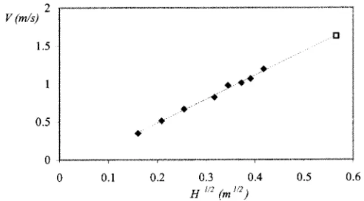
We measured the initial velocity of the liquid column as a function of the depth of immersion H. Since the dimension-less law at short time (tⰆ6) just reads z⫽t, introducing dimensional quantities implies a quick variation of the col-umn velocity with H. Then, Eq.共10兲 just is expressed as

Z共T兲⫽

冑

gHT. 共11兲

We did experiments with hexane, and found that indeed the height Z of the liquid column increases linearly with time at short time 共practically for t⬍1.5, which corresponds to 10 data points兲. Thus, we could report its velocity V as a func-tion of the square root of the depth height共Fig. 3兲, varying H from 2 to 35 cm, and indeed found a linear relation with a slope

冑

g, as predicted by Eq. 共11兲. Conservation of energy in Eq. 共3兲 for a system starting from z⫽0 also predicts a regime of constant velocity, but with a higher slope 共

冑

2g instead of

冑

g兲. Thus this regime of constant velocity also allows us to stress the existence of an energy loss in this system. Note also that the observed curve does not intercept the origin, which will be shown to be due to an entrance effect, characterized by a length of order R. Thus, our model only holds in the limit HⰇR.

FIG. 3. Rise velocity V of the liquid column at short time (t⬍1.5), as a function of the square root of H, the depth of immersion in water共closed diamonds兲 or in hexane 共open square兲. The full line has a slope冑g, as

More generally, Eqs.共6a兲 and 共6b兲 indicate that a solu-tion of constant velocity can only be found at the rise and if gravity can be neglected 共dz⬎0 and zⰆ1兲, or in the case where a horizontal pipe is connected with the bottom of a very large tank, which only generates an entrance flow. On the other hand, Eq. 共6b兲 shows that the velocity is never constant during the descent, and the only analytical regime in this case is a regime of constant acceleration: leaving a liquid column flow downwards from a very large height (z0Ⰷ1)

yields z¨⫽⫺1.

B. Oscillations, and their two regimes of damping At longer times, gravity cannot be neglected and Eqs. 共9a兲 and 共9b兲 can be integrated numerically. This solution is drawn in full line in Fig. 2, and compared with data obtained with hexane共for H⫽30 cm and R⫽1 cm兲.

The agreement between the theory and the experiment is excellent during the first oscillations: both the positions of the extrema and the periodicity are well predicted by the model. In particular, the first half-oscillation is the parabola derived in Eq. 共10兲. After typically ten oscillations, a slight shift appears, and the damping is observed to be quicker than predicted. We interpret this ‘‘overdamping’’ as due to the usual viscous friction along the tube, which must be taken into account as soon as a parabolic Poiseuille–Hagen profile has been established. This is achieved after the time neces-sary for the boundary layer to diffuse on a length R, which scales as␳R2/␩, with a numerical coefficient of order 0.11, as shown in Ref. 11. This time mainly depends on the tube radius, which can be easily checked by doing the same ex-periment in a thinner tube. Figure 4 shows the data obtained using a tube twice thinner (R⫽5 mm).

While the first oscillations remain quite well described by Eq.共9兲, it is indeed observed that the overdamping takes place much earlier: deviations toward Eq. 共9兲 are observed around t⫽15, instead of t⫽60 共in agreement with the scaling for the time of diffusion of the viscous boundary layer, in R2兲.

One of the remarkable features of this system is the per-sistence of the oscillations 共typically, more than 20 oscilla-tions can be observed兲. This is due to the particular source of

dissipation in Eq.共9兲. If the damping were just caused by the viscous dissipation along the pipe, this would provide a de-creasing exponential law for the maxima. In the case we are mainly interested in 共short time behavior兲, the damping is due to the singular pressure loss at the entrance 共or exit兲 of the pipe. The following argument allows us to understand why it is so low. From Eqs. 共3兲 and 共5兲, we can derive an equation for the energy loss:

d dt

共

zz˙

2_{⫹共z⫺1兲}2

兲

_{⫽⫺兩z˙兩z˙}2_{. 共12兲}

We set z(t)⫽1⫹␣(t)sin t, with ␣Ⰶ1, and suppose a slow variation for␣. During a period, the mean value of the quantities 兩z˙兩z˙2 and (zz˙2⫹(z⫺1)2) are 4兩␣3兩/3␲ and ␣2, respectively. Thus, an equation for the oscillation amplitude ␣ is obtained from Eq.共12兲:

d␣2 dt ⫽⫺ 4兩␣3兩 3␲ , 共13兲 which yields ␣共t兲⫽⫾3_2t␲. 共14兲

Even if this linear approximation should mainly concern the oscillations of small amplitude, it helps to understand that the damping is unusually long, due to this hyperbolic behavior. Furthermore, a hyperbolic damping is in fair agree-ment with our data even for oscillations of non-negligible amplitude, as shown in Fig. 5 where the maxima and minima corresponding to Fig. 2 are displayed versus time in a log– log plot.

It is observed that共apart from the first maximum兲, the damping is close to being hyperbolic in time 共the full line indicates the slope ⫺1兲, before accelerating 共the two last points兲, because of the additional dissipation due to the liq-uid viscosity. The latter can of course be evaluated by incor-porating in the model a viscous Poiseuille friction along the pipe. If the liquid front progresses by a length dz, the corre-sponding energy loss writes共in the same dimensionless vari-ables as previously兲

de⫽⫺⍀zz˙ dz, 共15兲

FIG. 4. Same experiment as in Fig. 2, in a thinner tube (R⫽5 mm). The dots are experimental data obtained with hexane. The full line corresponds to a numerical integration of Eq.共9兲, and the thin one to an integration of Eq.共17兲.

FIG. 5. Successive maxima␣M共triangles兲 and minima␣m共circles兲 of the

oscillation amplitude as a function of time. The data are taken from Fig. 2 and the full line has a slope⫺1.

where the number⍀ compares viscosity with inertia: ⍀⫽16␩H

1/2

␳R2g1/2. 共16兲

A difference with the energy loss due to pressure en-trance is that de共energy variation associated with a motion dz of the column兲 has the same expression whatever the di-rection of the motion, since z˙ and dz always have the same sign. Taking into account this viscous friction modifies Eq. 共6兲, which becomes

zz¨⫹z˙2⫽1⫺z⫺⍀zz˙ for dz⬎0, 共17a兲

zz¨⫽1⫺z⫺⍀zz˙ for dz⬍0. 共17b兲

Unlike Eq. 共6兲, Eq. 共17兲 cannot be integrated analyti-cally, but only numerically: such an integration is performed in Fig. 4共in thin line兲. The resulting curve fits quite well the extrema of the oscillations, but a shift in time appears, which remains unexplained. The use of a simple Poiseuille friction law for this oscillatory behavior could be questioned. The dissipation in the menisci could also become non-negligible in these regimes of approach of the equilibrium.

In the particular case of very large ⍀, inertia can be neglected, and the equation for the column motion simply is expressed as

⍀zz˙⫽1⫺z, 共18兲

which is often referred to, in the context of dynamic capillary rise, as the Washburn equation.12 At short time 共but large enough so that inertia can be neglected兲, z is small (zⰆ1), and integration of Eq. 共18兲 shows that the rise follows a diffusion-type law: z(t)⫽

冑

t/⍀. Then, when approaching equilibrium (z→1), we find an exponential relaxation: z(t) ⫽1⫺exp(⫺t/⍀).

An interesting feature of Eq.共17兲 is that it allows us to predict if the system will exhibit oscillations, or not. We saw that at large viscosities 共⍀Ⰷ1兲, the system just relaxes to-ward equilibrium, without any overshoot of the equilibrium height. Thus, a critical number ⍀_c does exist, below which oscillations develop. Close to ⍀_c, we can linearize Eqs. 共17a兲 and 共17b兲, which both reduce to

␨¨_⫹⍀␨˙_{⫹␨⫽0, 共19兲}

where we have set: z⫽1⫹␨, with␨Ⰶ1. This equation only leads to oscillations if⍀⬍⍀c⫽2, i.e., for small enough vis-cosities. Written dimensionally on the depth of immersion, this criterion reads

H⬍Hc⫽ ␳2_gR4

64␩2 . 共20兲

This criterion is largely fulfilled in the series of experiments presented previously: with water and centimetric tubes, Hc is of order 1 km! But this height rapidly decreases when making the tube thinner: for a tube of radius 3 mm and a liquid 10 times more viscous than water, Hc becomes of order 10 cm.

C. Very short time behavior

1. Starting of the liquid column

Let us come back to the beginning of the rise, starting from z⫽0. We showed that it obeys a very simple law, since the height of the column increases linearly with time 关Eq. 共11兲 and Fig. 2兴. An interesting question is the way the sys-tem finds its constant velocity V. At t⫽0, the system is at rest and there is a regime of transition during which the velocity quickly increases from 0 to V. Then, the column weight is negligible, and Eq. 共6a兲 can be written as

zz¨⫹z˙2⫽1. 共21兲

This equation has no solution which verifies both z⫽0 and z˙⫽0 for t⫽0, because of the singularity at z⫽0 关then, a zero velocity implies an infinite acceleration for Eq. 共21兲 to be obeyed兴. But physically, this singularity does not exist, be-cause of the mass of liquid entrained below the pipe. Thus, Eq.共21兲 can be rewritten, taking into account this additional mass from the beginning:

共z⫹z0兲z¨⫹z˙2⫽1, 共22兲

where z0 is the height below the pipe where the liquid is

entrained. Because the velocity field in the bath quickly van-ishes as a function of the distance to the entrance, we expect Z₀ 共the dimensional version of z₀兲 to be of order R, the radius of the tube. More precisely, by integrating the velocity profile from the entrance of the tube to infinity, Szekeley et al. 共in the context of capillarity兲13 calculated an entrance length Z₀⫽7/6R.

The general solution of Eq.共22兲 can be written as

z共t兲⫹z0⫽

冑

共a⫹z0兲2⫹t2 共23兲

denoting a⫽h/H as the height of liquid initially present in the tube 关as sketched in Fig. 1共a兲兴. At very short time, Eq. 共23兲 leads to a parabolic behavior 共acceleration stage兲:

z共t兲⬇a⫹ t

2

2共a⫹z₀兲. 共24兲

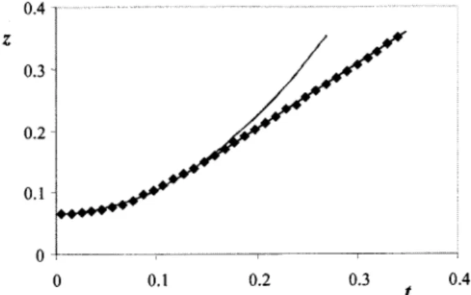
FIG. 6. Height z vs time t, in the very first steps of the rise共R⫽20 mm,

H⫽30 cm, and h⫽1.9 cm兲. The data, obtained with water, are successively

fitted by a parabola of equation z(t)⫽a⫹t2_/2(a⫹z

0) 关Eq. 共24兲兴, from which the coefficient z0can be deduced, and by a straight line of equation

Later (tⰇa⫹z₀), it matches the solution of constant velocity z⫽t analyzed previously 共Fig. 3兲.

By taking pictures at a high rate共typically 1000 frames per second兲, we could record the very beginning of the rise. Such data are reported in Fig. 6. It is observed that the be-havior at a very short time (t⬍0.15) can indeed be fitted by a parabola 关Eq. 共24兲兴, from which two coefficients can be deduced. One共a⫽0.064, in Fig. 6兲 is indeed found to be the initial height of liquid in the tube, while the second 共a⫹z0 ⫽0.126, in Fig. 6兲 provides the value of z0. Note that at

larger time, the parabolic regime meets the linear one dis-cussed in Sec. III A关Eq. 共11兲兴.

We plotted in Fig. 7 the value of Z0 共deduced from fits

such as the one in Fig. 6兲, as a function of R, the pipe radius. The results are found to agree closely with Szekeley’s predictions:13 Z0 varies linearly with R, with a numerical

coefficient of order 1.

We also considered the influence of h on Z0, and

fo-cused on the case of an empty tube (h→0). Then, as stressed previously, the problem should become singular. Practically, it is not; Fig. 8 shows that Z0does not depend on

h, which is consistent with the hypothesis of an added mass below the tube entrance. Even in the limit of a tube initially empty (h→0), the mass of accelerated fluid is not zero and the acceleration remains finite.

Since the flow inside the tube perturbs the reservoir on a length of order R, all the conclusions and interpretations pre-sented previously 共Secs. III A and III B兲, for which we had

ZⰇR, remain unchanged. The corrections mainly concern the very first steps of the trajectory, in the accelerating re-gime illustrated in Fig. 6. Other modifications are quite neg-ligible: for example, the position zM of the first maximum is found to be slightly modified by taking into account the en-trance length, from 1.5 to 1.5⫹z0/2共i.e., about 1.53 for the

data in Fig. 2, very close to the observed value兲. 2. Jet eruption

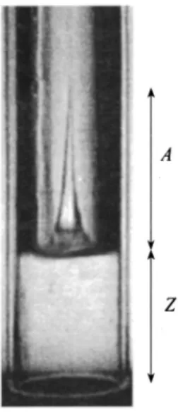
We have up to now focused our discussion on the motion of the whole column, but local deformations of the free sur-face were also observed at short time. Figure 9 shows a side view of the tube for Z of about 2R, where it can be seen that a liquid finger develops at the center of the tube. This finger rises during the first oscillation and collapses before z reaches its maximum value zM; this structure is local and does not impact the more macroscopic observations reported earlier.

The maximum size A of the finger depends on the height h of liquid initially in the tube, as shown in Fig. 10. Note that

FIG. 7. Entrance length Z0vs R, the radius of the tube共H⫽20 cm and h

⬇1 cm兲. The data are obtained with water.

FIG. 8. Entrance length Z0vs h the height of water initially present at the bottom of the pipe共R⫽1.2 cm and H⫽30 cm兲.

FIG. 9. Early stage of the rise共R⫽20 mm, H⫽30 cm, and h⫽0 mm兲. The front is flat, except at the tube center where a liquid共here, water兲 finger develops.

FIG. 10. Maximum amplitude of the water finger vs the initial height of liquid h. The experiment was carried out in a tube of radius R⫽20 mm and for H⫽30 cm.

h can even been made negative, by injecting air bubbles inside the empty pipe, before the rise takes place.

For large h共⬎6 mm兲, the size of the liquid finger does not depend on h. In this regime, we still observe some oscil-lations of the interface due to the abrupt contraction between the reservoir and the tube. Such oscillations were described by Taylor,14in the case of a tank with an oscillating wall. He showed that free standing waves could set up in the tank, with a shape very close to the one observed in the tube. For smaller h, a strong dependence can be observed: the smaller the height, the longer the finger. We were interested in the dynamics of the finger growth. Figure 11 reports different series of experiments.

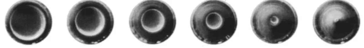
Besides the h dependence of A stressed previously, Fig. 11 shows that the finger grows after some delay 共typically 0.02 s兲, whatever h. This implies that a simple scenario 共ei-ther a convergence of the flow lines, or a kind of Rayleigh– Taylor instability due to the pulse of acceleration at the be-ginning of the rise兲 cannot explain the phenomenon. To go further, we took detailed films of the very beginning of the rise, focusing on the shape of the front interface. A series of snapshots taken at short time from above the tube is dis-played in Fig. 12.

These pictures show the existence of a circular rim, which sets near the wall of the tube, and closes as time goes on. The collapse of this surface wave produces a jet 共last picture of the series兲, as observed in similar situations.15The speed at which the liquid crater closes could be deduced from series similar to Fig. 12. Figure 13 shows how the diameter D of the liquid crater varies versus time.

The liquid crater closes at a constant velocity, which is 1.3 m/s in the abogiven example, of the order of the ve-locity

冑

gH of the rising column 共1.4 m/s, in the same ex-periment兲. Note that this wave starts propagating during the acceleration phase of the column. We saw that in this phase, the acceleration is of the order of gH/R 共for h⫽0兲,

signifi-cantly larger than g. Hence, for a wave vector k, a typical wave velocity should scale as

冑

gH/kR, of the order of

冑

gH for k⬃1/R. The time needed for shutting down the crater in a pipe of radius 20 mm is 26 ms, of the order of the delay measured in Fig. 11.

The origin of the crater can also be questioned, and re-lated to local flows at the pipe entrance. An effervescent drug placed below the tube provides indications on the flow: the gas bubbles reveal the existence of a circular vortex which remains close to the entrance as fluid sinks into the tube共Fig. 14兲. This vortex is related to the contraction of the flow lines entering the tube jet 共the so-called vena contracta phenom-enon兲, which traps some fluid at this place.

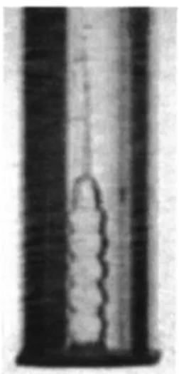
If h is negative, the initial conditions are different. Then, some air can be trapped in the tube creating a vortex ring of air rather than a liquid one 共as seen in the preceding para-graph兲. This phenomenon could be enhanced by placing a diaphragm at the tube entrance, as seen in Fig. 15. The col-umn then adopts the diameter of the diaphragm, with a modulation of frequency 184 Hz.共In addition, the finger pre-viously described is still here, above the main column, as observed in Fig. 15.兲 The column modulation is probably due to the stationary pressure waves of the air trapped into the tube. The frequency of such a resonant tube共open at one end and closed at the other兲 is

fn⫽nC/4Y, 共25兲

where C is the sound speed, Y the total length of the tube共1.6 m in the experiment兲, and n the mode of oscillation. For n ⫽1, we find f1⫽187 Hz, in very good agreement with the

measured frequency. This agreement remains excellent if the tube length is changed. Another cause of modulation of this cylindrical column of liquid could be the liquid surface ten-sion 共Plateau–Rayleigh instability兲, but it would lead to a FIG. 11. Amplitude of the water finger as a function of time共H⫽30 cm and

R⫽20 mm兲. The liquid column starts rising at T⫽0 and the finger starts

developing at the arrow.

FIG. 12. Set of pictures taken from above each 2.7 ms共R⫽20 mm, H⫽20 cm, and h⫽3 mm兲. These pictures correspond to the first points 共before the arrow兲 in Fig. 11. It can be observed that a cavity forms and closes, producing a water jet共last picture兲.

totally different wavelength 共higher than the column perim-eter, i.e., of the order of 10 cm instead of the observed cen-timeter in Fig. 15兲.

IV. CONCLUSION

We have studied the gravitational oscillations of a liquid column initially empty 共or nearly empty兲 and partially im-mersed inside a large reservoir. We have stressed that this problem has different analytical solutions, depending on the liquid viscosity. For very viscous liquids, the rise should obey the classical laws of impregnation共height proportional to the square root of time, followed by an exponential relax-ation toward equilibrium兲. But the interesting case is the low viscosity limit, for which different features were observed and analyzed, focusing in particular on the first steps of the rise共inertial regimes兲: after an accelerating phase 共where the

liquid entrained was mainly the one below the tube兲, the velocity of rise was found to be a constant fixed by the depth of immersion. Then, the rise was observed to slow down 共because of the column weight兲; we have shown that the trajectory is parabolic, reaching as a first maximum 1.5 times the depth of immersion. This value confirms that energy is indeed dissipated in this inertial phase, because of the sudden contraction endured by the moving liquid which passes from a large reservoir to a finite pipe. After this first maximum, many rebounds were observed, which was understood by evaluating the long range damping associated with this en-ergy loss: the envelope of the height/time dependence was found to be hyperbolic 共instead of exponential, as it is the case for usual viscous damping兲. At long time, viscosity must of course also be considered, which provides a quicker damping of the oscillations. We finally described qualita-tively an instability of the liquid/air interface during the first steps of the rise: then, a liquid jet is emitted while the col-umn develops. A complete study of this jet remains to be done.

ACKNOWLEDGMENTS

We thank Marc Rabaud, E´ lie Raphael, Konstantin Ko-rnev, and Alexander Neimark for very useful discussions.

1

D. Que´re´, E´ . Raphae¨l, and J. Y. Ollitrault, ‘‘Rebounds in a capillary tube,’’ Langmuir 15, 3679共1999兲.

2_{G. K. Batchelor, An Introduction to Fluid Dynamics共Cambridge}

Univer-sity Press, Cambridge, 1967兲.

3_{D. Bernoulli, Hydraulics共Dover, New York, 1968兲.} 4

A. B. Pandit and J. F. Davidson, ‘‘Hydrodynamics of the rupture of thin liquid films,’’ J. Fluid Mech. 212, 11共1990兲.

5_{G. I. Taylor, ‘‘The dynamics of thin sheets of fluid,’’ Proc. R. Soc. London,}

Ser. A 253, 313共1959兲.

6

F. E. C. Culick, ‘‘Comments on a ruptured soap film,’’ J. Appl. Phys. 31, 1128共1960兲.

7_{A. Buguin, L. Vovelle, and F. Brochard-Wyart, ‘‘Shocks in inertial}

dewet-ting,’’ Phys. Rev. Lett. 83, 1183共1999兲.

8_{D. Que´re´, ‘‘Inertial capillarity,’’ Europhys. Lett. 39, 533共1997兲.} 9

K. G. Kornev and A. V. Neimark, ‘‘Spontaneous penetration of liquids into capillaries and porous membranes revisited,’’ J. Colloid Interface Sci. 235, 101共2001兲.

10_{P. G. de Gennes, ‘‘Mechanics of soft interfaces,’’ Faraday Discuss. 104, 1}

共1996兲.

11

H. Schlichting, Boundary Layer Theory共McGraw–Hill, New York, 1968兲.

12_{E. W. Washburn, ‘‘The dynamics of capillary flow,’’ Phys. Rev. 17, 273}

共1921兲.

13_{J. Szekeley, A. W. Neumann, and Y. K. Chuang, ‘‘The rate of capillary}

penetration and the applicability of the Washburn equation,’’ J. Colloid Interface Sci. 35, 273共1971兲.

14_{G. I. Taylor, ‘‘An experimental study of standing waves,’’ Proc. R. Soc.}

London 218, 44共1953兲.

15_{B. W. Zeff, B. Kleber, J. Fineberg, and D. P. Lathrop, ‘‘Singularity}

dynam-ics in curvature collapse and jet eruption on a fluid surface,’’ Nature 共Lon-don兲 403, 401 共2000兲.

FIG. 14. Visualization of eddies using small bubbles as a tracer for the flow of water共R⫽20 mm and h⫽7 mm兲. The pictures are taken before the erup-tion of the jet.

FIG. 15. Water column rising in a tube (R⫽20 mm) where a diaphragm 共of radius 10 mm兲 partially closes the bottom.