Testing for parameter constancy in general causal time series models

HAL Id: hal-00561015

https://hal.archives-ouvertes.fr/hal-00561015v2

Submitted on 2 Jul 2011

HAL is a multi-disciplinary open access

archive for the deposit and dissemination of

sci-entific research documents, whether they are

pub-lished or not. The documents may come from

teaching and research institutions in France or

abroad, or from public or private research centers.

L’archive ouverte pluridisciplinaire HAL, est

destinée au dépôt et à la diffusion de documents

scientifiques de niveau recherche, publiés ou non,

émanant des établissements d’enseignement et de

recherche français ou étrangers, des laboratoires

publics ou privés.

series models

William Charky Kengne

To cite this version:

William Charky Kengne.

Testing for parameter constancy in general causal time series

mod-els.

Journal of Time Series Analysis, Wiley-Blackwell, 2012, 33, pp.503-518.

�10.1111/j.1467-9892.2012.00785.x�. �hal-00561015v2�

series models

July 2, 2011

by William Charky KENGNE1

SAMM, Universit´e Paris 1 Panth´eon-Sorbonne, 90 rue de Tolbiac 75634-Paris Cedex 13, France. E-mail: [email protected]

Abstract : We consider a process X = (Xt)t∈Z belonging to a large class of causal models including

AR(∞), ARCH(∞), TARCH(∞),... models. We assume that the model depends on a parameter θ0∈ IRdand consider the problem of testing for change in the parameter. Two statistics bQ(1)n and bQ(2)n are constructed using

quasi-likelihood estimator (QLME) of the parameter. Under the null hypothesis that there is no change, it is shown that each of these two statistics weakly converges to the supremum of the sum of the squares of inde-pendent Brownian bridges. Under the local alternative that there is one change, we show that the test statistic

b

Qn = max( bQ

(1)

n , bQ(2)n

)

diverges to infinity. Some simulation results for AR(1), ARCH(1) and GARCH(1,1) models are reported to show the applicability and the performance of our procedure with comparisons to some other approaches.

Keywords: Semi-parametric test; Change of parameters; Causal processes; Quasi-maximum likelihood

estimator; Weak convergence.

1

Introduction

Many statistical data can be represented by models which may change over time, for instance hydraulic flow, climate data. Before any inference on these data, it is crucial to test whether a change has not occurred in the model.

Since Page [23] in 1955, real advances have been done about tests for change detection. Horvath [11] pro-posed a test for detecting a change in the parameter of autoregressive processes based on weighted supremum and Lp-functionals of the residual sums. The CUSUM statistic which was introduced by Brown et al. [9] in

1975, was modified by Inclan and Tiao [13] for testing change in variance of independent random variables. Their test has asymptotically correct size but the asymptotic power is unknown. Numerous works devoted to the CUSUM-type procedure, for instance Kim et al. [15] for testing change in parameters of GARCH(1,1), Kokoszka and Leipus [17] in the specific case of ARCH(∞) or Aue et al. [1] for testing breaks in covariance.

1_{Supported by AUF (Agence Universitaire de la Francophonie) and Edulink ACP-EU project.}

Kulperger and Yu [18] studied the high moment partial sum process based on residuals and applied it to residual CUSUM test in GARCH model. Horv´ath et al. [12] suggested to compute the ratio of the CUSUM functionals instead of the differences for testing change in the mean of a time series. Berkes et al. [6] used a test based on approximate likelihood scores for testing parameter constancy in GARCH(p,q) models. These procedures are mostly developed in a parametric framework and their asymptotic powers are unknown. The present work is a new contribution to the challenging problem of test for change detection.

In this paper, we consider a general classMT(M, f ) of causal (non-anticipative) time series. Let M, f :

IRIN _{→ IR be measurable functions, (ξ}

t)t∈Z be a sequence of centered independent and identically distributed

(iid) random variables called the innovations and satisfying var(ξ0) = σ2 and Θ a compact subset of IRd. Let

T ⊂ Z, and for any θ ∈ Θ, define

ClassMT(Mθ, fθ): The process X = (Xt)t_∈Z belongs toMT(Mθ, fθ) if it satisfies the relation:

Xt+1= Mθ ( (Xt−i)i∈IN ) ξt+ fθ ( (Xt−i)i∈IN ) for all t∈ T . (1)

The existence and properties of this general class of affine processes were studied in Bardet and Wintenberger [2]. Numerous classical time series are included inMZ(M, f ): for instance AR(∞), ARCH(∞), TARCH(∞),

ARMA-GARCH or bilinear processes.

Now, assume that a trajectory (X1,· · · , Xn) of X = (Xt)t∈Z is observed and consider the following

hy-pothesis:

H0: there exists θ0∈ Θ such that (X1,· · · , Xn) belongs to the class M_{{1,··· ,n}}(Mθ0, fθ0) ;

H1 : there exist K ≥ 2, θ1,· · · , θK ∈ Θ such that (X1,· · · , Xn) belongs to K ∩ j=1 MTn j (Mθj, fθj) where Tn j ={tj−1+ 1, tj−1+ 2,· · · , tj} with 0 = t0< t1<· · · < tK−1< tK = n .

Thus, it is easy to see that under H1 the property of stationary is lost after the first change. This is not the case in many existing works (for instance Kouamo et al. [16] ) where the stationarity or the K-th order stationarity after the change is an essential assumption.

In this paper we study a new test for change detection (see Bardet et al. [3] for the procedure of the estimation of the instants of change). We consider a semi-parametric test statistic based on the QLME which is a modification of the statistic introduced by Lee et al. [19]. For k, k′ ∈ {2, · · · , n − 1} (with k ≤ k′) let bθn(Xk,· · · , Xk′) be the QLME of the parameter computed on {k, · · · , k′}. The basic idea of our procedure

is that : under H0, bθn(X1,· · · , Xk) and bθn(Xk+1,· · · , Xn) are close to bθn(X1,· · · , Xn) and the distances

∥bθn(X1,· · · , Xk)− bθn(X1,· · · , Xn)∥ and ∥bθn(Xk+1,· · · , Xn)− bθn(X1,· · · , Xn)∥ are not too large. Therefore,

we show that the test statistic is finite under the null hypothesis and diverges to infinity under the alternative of one change. Simulation results compared to some other procedures show that our procedure is more powerful. In Section 2 we present assumptions, some examples and construct the test statistic. In Section 3 we give some asymptotic results. The empirical studies of AR(1), ARCH(1) and GARCH(1,1) are detailed in Section 4 and the proofs of the main results are presented in Section 5.

2

Assumptions and test statistics

2.1

Assumptions on the class of models

M

(f

, M

)

Let θ ∈ IRd and Mθ and fθ be numerical functions such that for all (xi)i∈IN ∈ IRIN, Mθ

( (xi)i∈IN ) ̸= 0 and fθ ( (xi)i∈IN )

∈ IR. We will use the following norms:

1. ∥ · ∥ applied to a vector denotes the Euclidean norm of the vector; 2. for any compact set Θ⊆ IRd_{and for any g : Θ−→ IR}d′_,∥g∥

Θ= supθ∈Θ(∥g(θ)∥).

Let Ψθ= fθ, Mθ and i = 0, 1, 2, then for any compact set Θ⊆ IRd, define

Assumption Ai(Ψθ, Θ): Assume that ∥∂iΨθ(0)/∂θi∥Θ < ∞ and there exists a sequence of non-negative

real number (α(k)_i (Ψθ, Θ))i≥1 such that ∞ ∑ k=1 α(i)_k (Ψθ, Θ) <∞ satisfying ∂ i_Ψ θ(x) ∂θi − ∂iΨθ(y) ∂θi Θ≤ ∞ ∑ k=1

α_k(i)(Ψθ, Θ)|xk− yk| for all x, y ∈ IRIN.

In the sequel we refer to the particular case called ”ARCH-type process” if fθ = 0 and if the following

as-sumption holds with hθ:= Mθ2:

Assumption Ai(hθ, Θ): Assume that ∥∂ihθ(0)/∂θi∥Θ <∞ and there exists a sequence of non-negative real

number (α(k)_i (hθ, Θ))i≥1 such as ∞ ∑ k=1 α(i)_k (hθ, Θ) <∞ satisfying ∂ i_h θ(x) ∂θi − ∂ihθ(y) ∂θi Θ≤ ∞ ∑ k=1 α(i)_k (hθ, Θ)|x2k− y 2 k| for all x, y ∈ IR IN_.

Then define the set:

Θ(r) :={θ ∈ Θ, A0(fθ,{θ}) and A0(Mθ,{θ}) hold with

∑ k≥1 α(0)_k (fθ, θ) + (E|ξ0|r)1/r ∑ k≥1 α(0)_k (Mθ, θ) < 1}

∪ {θ ∈ Θ, fθ= 0 and A0(hθ,{θ}) hold with (E |ξ0|r)2/r ∑

k≥1

α(0)_k (hθ, θ) < 1}.

The Lipschitz-type hypothesis Ai(Ψθ, Θ) are classical when studying the existence of solutions of the general

model. If θ∈ Θ(r) the existence of a unique causal, stationary and ergodic solution X = (Xt)t_∈Z∈ MZ(fθ, Mθ)

is assured (see [2]). The subset Θ(r) is defined as a reunion to consider accurately general causal models and ARCH-type models simultaneously.

The following assumptions are needed to study QLME property.

Assumption D(Θ): ∃h > 0 such that inf

θ_∈Θ(|hθ(x)|) ≥ h for all x ∈ IR IN_.

Assumption Id(Θ): For all θ, θ′∈ Θ2_, (

fθ(X0, X−1,· · · ) = fθ′(X0, X−1,· · · ) and hθ(X0, X−1,· · · ) = hθ′(X0, X−1,· · · ) a.s. )

Assumption Var(Θ): For all θ∈ Θ, one of the families(∂fθ ∂θi(X0, X−1,· · · ) ) 1≤i≤d or (∂hθ ∂θi(X0, X−1,· · · ) ) 1≤i≤d is a.s. linearly independent.

As in [2], we will make the convention that if Ai(Mθ, Θ) holds then α

(i)

ℓ (hθ, Θ) = 0 and if Ai(hθ, Θ) holds

then α(i)_ℓ (Mθ, Θ) = 0. Denote :

Assumption K(fθ, Mθ, Θ) : for i= 0, 1, 2, Ai(fθ, Θ) and Ai(Mθ, Θ) (or Ai(hθ, Θ)) hold and there exists

l > 2 such that α(i)_j (fθ, Θ) + α

(i)

j (Mθ, Θ) + α

(i)

j (hθ, Θ) =O(j−l), for i= 0, 1.

Throughout the sequel, we will assume that the functions θ 7→ Mθ and θ 7→ fθ are twice continuously

differentiable on Θ.

2.2

Examples

Consider the AR(∞) process defined by :

Xt=

∑

k≥1

ϕk(θ∗0)Xt−k+ ξt , t∈ Z

with θ∗₀∈ Θ, where Θ is a compact subset of IRd _{such that}∑

k≥1∥ϕk(θ)∥Θ< 1. The process belongs to

the classMZ(Mθ∗₀, fθ∗₀) where fθ(x1,· · · ) = ∑

k≥1ϕk(θ)xk and Mθ≡ 1 for all θ ∈ Θ. Then Assumptions

D(Θ) and A0(fθ, Θ) hold with h = 1 and α

(0)

k (fθ, Θ) =∥ϕk(θ)∥Θ. If there exists ℓ > 2 and ϕk twice

differentiable such as ∥ϕk(θ)∥Θ = ∥ϕ′k(θ)∥Θ = ∥ϕ′′k(θ)∥Θ = O(k−ℓ), then Assumptions K(fθ, Mθ, Θ)

holds. Moreover, if ξ0 is a nondegenerate random variable, Id(Θ) and Var(Θ) hold. For any r≥ 1 such that E|ξ0|r<∞, Θ(r) = Θ.

2. GARCH(p,q) models.

Consider the GARCH(p,q) process defined by :

Xt= σtξt, σt2= α∗0+ q ∑ k=1 α∗_kX_t2_−k+ p ∑ k=1 β∗_kσ2_t−k , t∈ Z with E (ξ2

0) = 1 and θ∗0:= (α∗0,· · · , αq∗, β∗1,· · · , βp∗)∈ Θ where Θ is a compact subset of ]0, ∞[×[0, ∞[p+q

such that ∑q_k=1αk +

∑p

k=1βk < 1 for all θ ∈ Θ. Then there exists (see Bollerslev [8] or Nelson

and Cao [22]) a nonnegative sequence (ψk(θ∗0))k≥0 such that σ2t = ψ0(θ∗0) + ∑ k_≥1ψk(θ∗0)X 2 t−k with ψ0(θ∗0) = α∗0/(1− ∑p

k=1β∗k). This process belongs to a class MZ(Mθ₀∗, fθ∗₀) where Mθ(x1,· · · ) = √

ψ0(θ) + ∑

k≥1ψk(θ)xk and fθ ≡ 0 ∀θ ∈ Θ. Assumptions D(Θ) holds with h = inf

θ∈Θ(α0). If there

exists 0 < ρ0< 1 such that for any θ∈ Θ, ∑q

k=1αk+

∑p

k=1βk ≤ ρ0 then the sequences (∥ψk(θ)∥Θ)k≥1,

(∥ψ′_k(θ)∥Θ)k≥1 and (∥ψk′′(θ)∥Θ)k≥1 decay exponentially fast (see Berkes et al. [5]), thus Assumption

K(fθ, Mθ, Θ) holds. Moreover, if ξ20 is a nondegenerate random variable, Id(Θ) and Var(Θ) hold. For

r≥ 2 denote Θ(r) ={θ∈ Θ ; (E |ξ0|r)2/r q ∑ k=1 αk+ p ∑ k=1 βk < 1 } .

2.3

Test statistics

Assume that a trajectory (X1,· · · , Xn) is observed. It is clear that if (X1,· · · , Xn)∈ M{1,··· ,n}(Mθ, fθ), then

for T ⊂ {1, · · · , n}, the conditional quasi-(log)likelihood computed on T is given by :

Ln(T, θ) :=− 1 2 ∑ t_∈T qt(θ) with qt(θ) = (Xt− fθt) 2 ht θ + log(ht_θ) where ft θ = fθ ( Xt₋₁, Xt₋₂. . . ) , Mt θ = Mθ ( Xt₋₁, Xt₋₂. . . ) and ht θ = Mθt 2

. Therefore, we approximate the conditional log-likelihood with :

bLn(T, θ) :=− 1 2 ∑ t_∈T bqt(θ) where bqt(θ) := ( Xt− bfθt )2 bht θ + log(bht_θ) with bft θ= fθ ( Xt−1, . . . , X1, 0, 0,· · · ) , cMt θ= Mθ ( Xt−1, . . . , X1, 0, 0,· · · ) and bht θ= ( cM t θ) 2_. For T ⊂ {1, · · · , n}, define the estimator bθn(T ) := argmax

θ∈Θ

( bLn(T, θ)). Moreover, for 1 ≤ k ≤ n, denote

Tk={1, · · · , k} and Tk ={k + 1, · · · , n}. Now, define b Gn(T ) := 1 Card(T ) ∑ t∈T (_∂bq t(bθn(T )) ∂θ )(_∂bq t(bθn(T )) ∂θ )_′ and bFn(T ) :=− 2 Card(T ) (_∂2bL n(T, bθn(T )) ∂θ∂θ′ ) . For k = 1,· · · , n − 1, denote : bΣn,k:= k nFbn(Tk) bGn(Tk) −1_Fb n(Tk)1_{det( bGn(Tk))̸=0}+ n− k n Fbn(Tk) bGn(Tk) −1_Fb n(Tk)1_{det( bGn(Tk))̸=0}.

Let (vn)n_∈IN be a sequence satisfying vn → ∞ and vn/n→ 0 (as n → ∞). Denote Πn= [vn, n− vn]∩ IN and

define the statistics: b Q(1)n := max k_∈Πn b Q(1)_n,k where bQ(1)_n,k := k 2 n(bθn(Tk)− bθn(Tn) )_′bΣ n,k(bθn(Tk)− bθn(Tn) ) ; b Q(2)n := max k∈Πn b Q(2)_n,k where bQ(2)_n,k := (n− k) 2 n (bθn(Tk)− bθn(Tn) )_′bΣ n,k(bθn(Tk)− bθn(Tn) ) ; b Qn := max( bQ (1) n , bQ(2)n )

which is the test statistic.

Remark 2.1 Note that, the choice of (vn) is crucial in practice. We evaluated the procedure with vn =

[log n], [(log n)2_{], [(log n)}3_{] and recommend to use v}

n = [(log n)2] for linear model and vn = [(log n)5/2] for

GARCH-type model.

Lee and Song [21] constructed a test for detecting changes in parameters of ARMA-GARCH models. Their test statistic uses a matrix bΣn which depends on the estimator bθn(Tn). Under the null hypothesis (the

pa-rameter θ0does not change), bΣn is a consistent estimator of F G−1F where G = E [(∂q0(θ0)/∂θ)(∂q0(θ0)/∂θ)′] and F = E [∂2_q

0(θ0)/∂θ∂θ′]. Under the alternative, the model depends on several parameters and bθn(Tn) may

not be a consistent estimator of one of them. Therefore, the convergence of the matrix bΣn is not assured.

introduce the family of matrices{bΣn,k, k∈ Πn}. It is easy to see that under the null hypothesis, any sequence

(bΣn,kn)n>1,kn∈Πn is consistent. We show (see proof of Theorem 3.2) that under the local alternative where

there is one change in the model, there exists a sequence (bΣn,k∗_n)n>1,k_n∗_∈Πn which converges.

3

Asymptotic results

3.1

Asymptotic under the null hypothesis

Theorem 3.1 Assume D(Θ), Id(Θ), Var and K(fθ, Mθ, Θ). Under the null hypothesis H0, if θ0 ∈

◦ Θ(4), then for j = 1, 2, b Q(j)n −→D n→∞ sup 0_≤τ≤1∥W d(τ )∥2

where Wd is a d-dimensional Brownian bridge.

For any α∈ (0, 1), let Cαdenote the (1− α/2)-quantile of the distribution of sup

0≤τ≤1

∥Wd(τ )∥2. Then, the

following corollary is a direct application of Theorem 3.1.

Corollary 3.1 Under assumptions of Theorem 3.1 :

∀α ∈ (0, 1) lim sup

n→∞

P( bQn > Cα

)

≤ α.

Remark 3.1 Quantile values of the distribution of sup

0≤τ≤1∥W

d(τ )∥2 are known (see for instance Kieffer [14]

for d∈ {1, · · · , 5} or Lee et al. [19] for d ∈ {1, · · · , 10}).

Theorem 3.1 and Corollary 3.1 imply that a large value of bQn means there is a change in the model. At a

nominal level α, the critical region of the test is ( bQn > Cα).

Figure 1 is an illustration of the test procedure for AR(1) process. At a level α = 0.05, for d = 1, Cα≃ 2.20.

Figure 1 a-) and b-) show that, the values of bQ(1)_n,k and bQ(2)_n,k are all below the red line which represents the limit of the critical region. Figure 1 c-) and d-) show that bQ(1)_n,k and bQ(2)_n,k are larger and increase around the point where the change occurs.

As it can be observed on the Figure 1 and Figure 2 , the statistics bQ(1)n and bQ

(1)

n are not clearly equal.

Figure 2 shows the typical example for ARCH(1) with one change where bQ(1)n < Cα and bQ

(2)

n > Cα. In

general, we don’t know if under the alternative hypothesis each of statistics bQ(1)n and bQ(2)n take large values.

But, under the local alternative of one change, the maximum of these two statistics diverges to infinity (see Theorem 3.2). This is the reason why we define the critical region as{max( bQ(1)n , bQ(2)n ) > Cα}.

3.2

The asymptotic under a local alternative

In this subsection, we consider a local alternative that there is one change in the model. More precisely, define

H₁(loc): there exist τ∗∈ (0, 1) and θ∗1, θ∗2∈ Θ with θ∗1̸= θ∗2 such that X1,· · · X[nτ∗]∈ MT[nτ ∗ ](Mθ∗1, fθ∗1) and X[nτ∗]+1,· · · , Xn∈ MT[nτ ∗ ](Mθ∗2, fθ∗2).

Theorem 3.2 Assume D(Θ), Id(Θ), Var and K(fθ, Mθ, Θ). Under H (loc) 1 , if θ1∗, θ2∗∈ ◦ Θ(4), then b Qn a.s. −→ n→∞ ∞.

Remark 3.2 1-) Theorem 3.2 shows that the test with the local alternative H₁(loc) is consistent in power. 2-) This procedure can also be used to test multiple changes using ICSS type algorithm developed by Incl´an and Tiao [13].

a−) Qn,k(

1)

for AR(1) with no change

Time 0 200 400 600 800 1000 0.0 0.5 1.0 1.5 2.0 b−) Qn,k( 2)

for AR(1) with no change

Time 0 200 400 600 800 1000 0.0 0.5 1.0 1.5 2.0 c−) Qn,k (1)

for AR(1) with one change at k* = 400

Time 0 200 400 600 800 1000 0 1 2 3 4 5 d−) Qn,k (2)

for AR(1) with one change at k* = 400

Time 0 200 400 600 800 1000 0 1 2 3 4

Figure 1 : Typical realization of the statistics bQ(1)_n,k and bQ(2)_n,k for 1000 sample of AR(1) with vn = [log n]. a-)

and b-) are the case of AR(1) where parameter ϕ1= 0.3 remains constant. c-) and d-) are the case of AR(1) with parameter ϕ1= 0.3 changing to 0.5 at k∗= 400.

a−) Qn,k( 1)

for ARCH(1) with one change at k* = 400

Time 0 200 400 600 800 1000 0 1 2 3 4 b−) Qn,k( 2)

for ARCH(1) with one change at k* = 400

Time 0 200 400 600 800 1000 0 1 2 3 4

Figure 2 : Typical realization of the statistics bQ(1)_n,kand bQ(2)_n,kfor 1000 sample of ARCH(1) with vn= [(log n)2].

a-) and b-) are the case of ARCH(1) with parameter θ1= (1, 0.3) changing to (1, 0.15) at k∗= 400.

4

Some simulations results

In this section, we evaluate the performance of the procedure through empirical study. We compare our results with those obtained by Kouamo et al. [16], Lee and Na [20] and the results obtained from the residual CUSUM test by using the statistics defined by Kulperger and Yu [18]. For a sample size n, bQn is computed

with vn= [(ln n)2] for AR model and vn= [(ln n)5/2] for GARCH model and is compared to the critical value

of the test. In the following models, (ξt)t∈Z are iid standard Gaussian random variables.

4.1

Test for parameter change in AR(p) models

p

∑

k=1

ϕ∗_kXt−k+ ξtwith p∈ IN∗. The true parameter of the model is

de-noted by θ∗0 = (ϕ∗1,· · · , ϕ∗p)∈ Θ where Θ = {θ = (ϕ1,· · · , ϕp)∈ IRp / p

∑

i=1

|ϕi| < 1}. Since Mθ≡ 1, Θ(r) = Θ

for any r ≥ 1. Assume (X1,· · · , Xn) is observed, we have for any θ ∈ Θ, bqt(θ) =

( Xt− p ∑ k=1 ϕkXt−k )2 , ∂bqt(θ) ∂θ =−2 ( Xt− p ∑ k=1 ϕkXt−k ) · (Xt−1, Xt−2,· · · , Xt−p) and for 1≤ i, j ≤ n ∂2_bq t(θ) ∂ϕi∂ϕj = 2Xt−iXt−j.

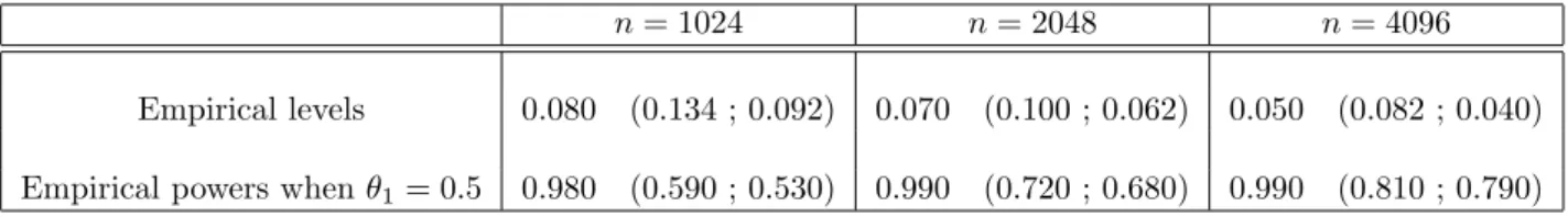
We consider a AR(1) process with one parameter. At level α = 0.05, the critical value is Cα≃ 2.20. For

n = 1024, 2048, 4096 ; we generate a sample (X1,· · · , Xn) in the following situations : (i) there is no change

θ1= 0.5 at n/2. The following table indicates the proportion of the number of rejections of the null hypothesis out of 100 repetitions.

n = 1024 n = 2048 n = 4096

Empirical levels 0.080 (0.134 ; 0.092) 0.070 (0.100 ; 0.062) 0.050 (0.082 ; 0.040) Empirical powers when θ1= 0.5 0.980 (0.590 ; 0.530) 0.990 (0.720 ; 0.680) 0.990 (0.810 ; 0.790) Table 1: Empirical levels and powers at nominal level 0.05 of the test for parameter change in AR(1) model. The empirical

levels are computed when θ0= 0.9 ; the empirical powers are computed when θ0changes to θ1= 0.5 at n/2. Figures in brackets

are the results obtained by Kouamo et al. [16] at the scale J=4 with KSM and CVM statistic in wavelet domain.

Table 1 shows that the empirical level of the test decreases as n increases and equals to 0.05 when n = 4096. These levels are close to those obtained by Kouamo et al. with CVM (Cram´er-Von Mises) test statistic. The results obtained with our test statistic bQn are clearly more accurate.

4.2

Test for parameter change in GARCH(1,1) models

∀t ∈ Z, Xt= σtξt with σt2= α∗0+ α∗1X 2

t−1+ β1∗σ 2

t−1

with θ∗₀ = (α₀∗, α∗₁, β₁∗) ∈ Θ ⊂]0, ∞[×[0, ∞[2 and satisfying α∗₁+ β₁∗ < 1. The ARCH(∞) representation is σ2

t = α0∗/(1− β1∗) + α∗1 ∑

k≥1

(β₁∗)k−1_X2

t−k. For any θ∈ Θ and t = 2, · · · , n , we have

bht θ= α0/(1− β1) + α1Xt2₋₁+ α1 t ∑ k=2 β₁k−1Xt2_−k and bqt(θ) = Xt2/ bhtθ+ log(bhtθ).

Therefore, it follows that ∂bqt(θ)

∂θ = 1 bht θ ( 1− X 2 t bht θ )(_∂bht θ ∂α0 ,∂bh t θ ∂α1 ,∂bh t θ ∂β1 ) with ∂bht_θ/∂α1 = Xt2−1 + t ∑ k=2 βk₁−1X_t2_−k ∂bht θ/∂α0= 1/(1− β1), and ∂bhtθ/∂β1= α0/(1− β1)2+ α1Xt2−2+ α1 t ∑ k=3 (k− 1)β₁k−2X2 t_−k.

Let θ = (α0, α1, β1) = (θ1, θ2, θ3)∈ Θ, for 1 ≤ i, j ≤ 3, we have

∂2_bq t(θ) ∂θi∂θj = 1 (bht θ)2 (_2X2 t bht θ − 1)∂bhtθ ∂θi ∂bht θ ∂θj + 1 bht θ ( 1−X 2 t bht θ ) _∂2bht θ ∂θi∂θj with ∂2bht_θ/∂α02 = 0, ∂2bhtθ/∂α0∂α1 = 0, ∂2bhtθ/∂α 2 1 = 0, ∂2bhtθ/∂α1∂β1 = Xt2₋₂ + t ∑ k=3 (k− 1)β₁k−2X_t2_−k, ∂2bht θ/∂α0∂β1= 1/(1− β1)2 and ∂bhtθ/∂β 2 1 = 2α0/(1− β1)3+ 2α1Xt2−3+ α1 t ∑ k=4 (k− 1)(k − 2)βk₁−3X2 t−k.

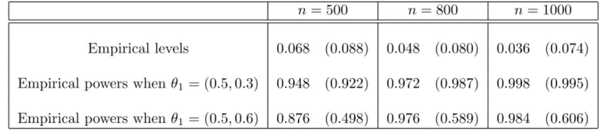
1. Case of ARCH(1). Assume β1= 0 and θ = (α0, α1). At level α = 0.05, the critical value is Cα ≃ 3.02.

For n = 500, 800, 1000 ; we generate a sample (X1,· · · , Xn) in the following situations : (i) there is

no change, the parameter of the model is θ0 = (1, 0.3) and (ii) there is one change, the parameter

θ0= (1, 0.3) changes to two different values of θ1= (0.5, 0.3) and θ1= (0.5, 0.6) at n/2. The following table indicates the proportion of the number of rejections of the null hypothesis out of 500 repetitions.

n = 500 n = 800 n = 1000

Empirical levels 0.068 (0.088) 0.048 (0.080) 0.036 (0.074) Empirical powers when θ1= (0.5, 0.3) 0.948 (0.922) 0.972 (0.987) 0.998 (0.995) Empirical powers when θ1= (0.5, 0.6) 0.876 (0.498) 0.976 (0.589) 0.984 (0.606)

Table 2: Empirical levels and powers at nominal level 0.05 of the test for parameter change in ARCH(1) model. The empirical

levels are computed when θ0= (1, 0.3) ; the empirical powers are computed when θ0changes to θ1 at n/2. Figures in brackets

are the results obtained by Lee and Na [20].

2. Case of GARCH(1,1). Now θ = (α0, α1, β1). At level α = 0.05, the critical value is Cα ≃ 3.47. For

n = 500, 1000, 1500 ; we generate a sample (X1,· · · , Xn) in the following situations : (i) there is no

change, the parameter of the model is θ0 = (1, 0.4, 0.1) and (ii) there is one change, the parameter

θ0 = (1, 0.4, 0.1) changes two different values of θ1 = (0.7, 0.4, 0.1) and θ1 = (1, 0.4, 0.3) at n/2. The following table indicates the proportion of the number of rejections of the null hypothesis out of 500 repetitions.

n = 500 n = 1000 n = 1500

Empirical levels 0.100 (0.030) 0.078 (0.032) 0.052 (0.042) Empirical powers when θ1= (0.7, 0.4, 0.1) 0.498 (0.334) 0.752 (0.658) 0.934 (0.848) Empirical powers when θ1= (1, 0.4, 0.3) 0.654 (0.404) 0.968 (0.772) 0.976 (0.922)

Table 3: Empirical levels and powers at nominal level 0.05 of test the for parameter change in GARCH(1,1) model. The empirical

levels are computed when θ0= (1, 0.4, 0.1) ; the empirical powers are computed when θ0changes to θ1at n/2. Figures in brackets

are the results of the residual CUSUM test using CU SU M(2)_{statistic defined by Kulperger and Yu [18].}

Table 2 and Table 3 show that the empirical level of the test decreases and the empirical power increases as n increases. For ARCH model, we can see that the empirical level is less than 0.05 when n = 800. It is not very surprising because the asymptotic size of the test is less than α = 0.05. This is not the case for GARCH model. It is explained by the fact that the application of the procedure to GARCH model requires ARCH(∞) representation. Thus, the information contained in all the past of the process is not used because it is not observed. In Table 2, figures in brackets are the results obtained by Lee and Na [20] using the CUSUM test based on conditional least-squares estimator. In Table 3, figures in brackets are the results of the residual CUSUM test that we obtained by using CU SU M(2) _{statistic studied by Kulperger and Yu [18]. Once again,} our test statistic bQn provides best results.

5

Proofs of the main results

Let (ψn)n and (rn)n be sequences of random variables. Throughout this section, we use the notation ψn =

oP(rn) to mean : for all ε > 0, P (|ψn| ≥ ε|rn|) → 0 as n → ∞. Write ψn = OP(rn) to mean : for all ε > 0,

5.1

Some preliminary results

Under the null hypothesis H0 the observations (X1,· · · , Xn) belong in the classM_{{1,··· ,n}}(Mθ0, fθ0), de-fine the matrix G := E

[_∂q 0(θ0) ∂θ ∂q0(θ0) ∂θ ′]

( where ′ denotes the transpose) and F := E [_∂2_q

0(θ0)

∂θ∂θ′

]

. Under

assumption Var, F is a non-singular matrix (see [2]).

Lemma 5.1 Assume the functions θ7→ Mθ and θ7→ fθ are 2-times continuously differentiable on Θ. Under

the null hypothesis D(Θ) and Var, G is a symmetric, positive definite matrix.

Proof. It is clear that G is symmetric. Moreover, for 1≤ i ≤ d, we have :

∂q0(θ0) ∂θi =−2√ξ0 h0 θ0 ∂f0 θ0 ∂θi − ξ20 h0 θ0 ∂h0 θ0 ∂θi + 1 h0 θ0 ∂h0 θ0 ∂θi

. Thus, using independence of ξ0and X₋₁, X₋₂,· · · we obtain : E [_∂q0(θ0) ∂θ ′_∂q 0(θ0) ∂θ ] = 4E [ ₁ h0 θ0 ∂f0 θ0 ∂θ ′_∂f0 θ0 ∂θ ] + E ( (ξ2₀− 1)2 ) E [ ₁ (h0 θ0) 2 ∂h0 θ0 ∂θ ′_∂h0 θ0 ∂θ ] . (2) Since E ξ2

0 = 1, it is easy to see that E (

(ξ2 0− 1)2

)

> 0.

Under Var, one of the two matrix of the right-hand side of relation (2) is positive definite and the other is semi-positive definite. Thus, G is positive definite.

Now, recall that F := E [_∂2_q

0(θ0)

∂θ∂θ′

]

. Let T ⊂ {1, · · · , n}. For any θ ∈ Θ and i = 1, · · · , d, by Taylor expansion of ∂Ln(T, θ0)/∂θi, there exist θn,i∈ [θ0, θ] such that:

∂Ln(T, θ) ∂θi = ∂Ln(T, θ0) ∂θi +∂ 2_L n(T, θn,i) ∂θ∂θi (θ− θ0) (3)

where [a, b] = {λa + (1 − λ)b ; λ ∈ [0, 1]}. Denote Fn(T, θ) = −2

( 1 card(T ) ∂2Ln(T, θn,i) ∂θ∂θi ) 1≤i≤d. Then, (3) implies, Card(T )Fn(T, θ)(θ− θ0) =−2 (∂Ln(T, θ) ∂θ − ∂Ln(T, θ0) ∂θ ) . (4)

Similarly, for any θ∈ Θ we can find a matrix eFn(T, θ) such that

Card(T ) eFn(T, θ)(θ− θ0) =−2 (∂ bLn(T, θ) ∂θ − ∂ bLn(T, θ0) ∂θ ) . (5)

With θ = bθn(T ) in (5) and using the fact that ∂ bLn(T, bθn(T ))/∂θ = 0 (because bθn(T ) is a local extremum of

bLn(T,·)), it comes Card(T ) eFn(T, bθn(T ))(bθn(T )− θ0) = 2 ∂ bLn(T, θ0) ∂θ . (6) Remark 5.1 If Card(T ) −→ n→∞ ∞ and θ = θ(n) −→n→∞ θ0, then Fn(T, θ) a.s. −→ n→∞ F and eFn(T, θ) a.s. −→ n→∞ F (see [2] and [3]). In particular, if Card(T ) −→

n→∞ ∞ , then Fn (T, bθn(T )) a.s. −→ n→∞ F and eFn(T, bθn(T )) a.s. −→ n→∞ F.

Lemma 5.2 Under assumptions of Theorem 3.1

1 √ n kmax∈Πn k( eFn(Tk, bθn(Tk))− F ) (bθn(Tk)− θ0) = oP(1).

Proof. For k ∈ Πn, we know that

√

k(bθn(Tk))− θ0) converges in distribution to the Gaussian law as

n −→ ∞ (see Theorem 2 of [2]). Therefore, max

k∈Πn

√k(bθn(Tk)− θ0) = OP(1). Remark 5.1 implies that

max

k∈Πn

eFn(Tk, bθn(Tk))− F = o(1) a.s. Thus

1 √ n kmax_∈Πn k( eFn(Tk, bθn(Tk))− F ) (bθn(Tk)− θ0) ≤ max k_∈Πn eFn(Tk, bθn(Tk))− F ×max k_∈Πn √k(bθn(Tk)− θ0) = o(1)OP(1) a.s. = oP(1).

Under assumptions of Theorem 3.1, the matrix G is invertible. Denote Σ = F G−1F Q(1)_n := max k_∈Πn Q(1)_n,k where Q(1)_n,k := k 2 n(bθn(Tk)− bθn(Tn) )_′Σ(b θn(Tk)− bθn(Tn) ) and Q(2)n := max k_∈Πn Q(2)_n,k where Q(2)_n,k :=(n− k) 2 n (bθn(Tk)− bθn(Tn) )′Σ(b θn(Tk)− bθn(Tn) ) .

Lemma 5.3 Under assumptions of Theorem 3.1

max

k∈Πn

 bQ(j)_n,k− Q(j)_n,k= oP(1) for j = 1, 2.

Proof. The proof is provided for j = 1, proceed similarly for j = 2. For any k∈ Πn, we have

 bQ(1)_n,k− Q(1)_n,k ≤ k 2 n∥bθn(Tk)− bθn(Tn)∥ 2_∥bΣ n,k− Σ∥ ≤ 2k2 n ( ∥bθn(Tk)− θ0∥2+∥bθn(Tn)− θ0∥2 ) ∥bΣn,k− Σ∥ ≤ 2(∥√k(bθn(Tk)− θ0)∥2+∥ √ n(bθn(Tn)− θ0)∥2 ) ∥bΣn,k− Σ∥. (7) Since k∈ Πn, k, n−k −→ ∞ as n −→ ∞. Therefore, √ k(bθn(Tk)−θ0) = OP(1) as n−→ ∞, √ n(bθn(Tn)−θ0) = OP(1), bFn(Tk) a.s. −→ n→∞ F , bFn(Tk) a.s. −→ n→∞ F , bGn(Tk) a.s. −→ n→∞ G and bGn(Tk) a.s. −→ n→∞

G which is invertible. Thus, for

n large enough, bGn(Tk) and bGn(Tk) are invertible. It follows that as n−→ ∞,

∥bΣn,k− Σ∥ = k nFbn(Tk) bGn(Tk) −1_Fb n(Tk) + n− k n Fbn(Tk) bGn(Tk) −1_Fb n(Tk)− F G−1F = k n ( k nFbn(Tk) bGn(Tk) −1_Fb n(Tk)− F G−1F ) +n− k n ( bFn(Tk) bGn(Tk) −1_Fb n(Tk)− F G−1F) ≤ ∥ bFn(Tk) bGn(Tk)−1Fbn(Tk)− F G−1F∥ + ∥ bFn(Tk) bGn(Tk)−1Fbn(Tk)− F G−1F∥ = o(1) a.s.

Therefore, (7) implies max

k_∈Πn

 bQ(1)_n,k− Q(1)_n,k= oP(1).

Lemma 5.4 Under assumptions of Theorem 3.1

−2 √ n ∂Ln(T[nτ ], θ0) ∂θ D −→ WG(τ ) in D([0, 1], IRd)

Proof. Recall that −2∂Ln(T[nτ ], θ0)

∂θ =

[nτ ]∑

t=1

∂qt(θ0)

∂θ . Denote Ft= σ(Xt−1,· · · ). Since X is stationary and

ergodic, it is the same for the process (∂qt(θ0)

∂θ )t∈Z. Moreover, ( ∂qt(θ0)

∂θ ,Ft) is a square integrable martingale

difference process (see [2]) with covariance matrix G. Then, the result follow by using Theorem 23.1 Billingsley (1968) (see [7] page 206).

Lemma 5.5 Under assumptions of Theorem 3.1

−2 √ nG −1/2(∂Ln(T[nτ ], θ0) ∂θ − [nτ ] n ∂Ln(Tn, θ0) ∂θ ) D −→ Wd(τ ) in D([0, 1], IRd)

where Wd is a d-dimensional Brownian bridge.

Proof. By Lemma 5.4, it comes

−2 √ n (∂Ln(T[nτ ], θ0) ∂θ − [nτ ] n ∂Ln(Tn, θ0) ∂θ ) D −→ WG(τ )− τWG(1) in D([0, 1], IRd).

Since the covariance matrix of the process{WG(τ )− τWG(1), 0≤ τ ≤ 1} is (min(τ, s) − τs)G, the covariance

matrix of the process{G−1/2(WG(τ )−τWG(1)), 0≤ τ ≤ 1} is (min(τ, s)−τs)Id(where Idis the d-dimensional

identity matrix). Therefore, the process is equal (in distribution) to a d-dimensional Brownian bridge and the result follows.

Lemma 5.6 Under assumptions of Theorem 3.1

−2 √ nG −1/2∂ bLn(T[nτ ], bθn(Tn)) ∂θ D −→ Wd(τ ) in D([0, 1], IRd).

Proof. From [2], we have √1

n ∂L n(Tn,·) ∂θ − ∂ bLn(Tn,·) ∂θ Θ= oP(1). This implies, 1 √ n kmax∈Πn ∂Ln(Tk,·) ∂θ − ∂ bLn(Tk,·) ∂θ Θ= oP(1). (8)

Let k∈ Πn. Applying (4) with T = Tk and θ = bθn(Tn), we have

kFn(Tk, bθn(Tn))(bθn(Tn)− θ0) =−2 (∂Ln(Tk, bθn(Tn)) ∂θ − ∂Ln(Tk, θ0) ∂θ ) . By plugging it in (8), we have 1 √ n kmax∈Πn ∂bLn(Tk, bθn(Tn)) ∂θ − ∂Ln(Tk, θ0) ∂θ + 1 2kFn(Tk, bθn(Tn))(bθn(Tn)− θ0) = oP(1). (9) But, by Remark 5.1, it comes that

1 √ n kmax∈Πn k(Fn(Tk, bθn(Tn))− Fn(Tn, bθn(Tn)) ) (bθn(Tn)− θ0) ≤ √1 n kmax∈Πn k(Fn(Tk, bθn(Tn))− Fn(Tn, bθn(Tn))) × ∥√n(bθn(Tn)− θ0)∥ = o(1)OP(1) a.s. = oP(1).

Thus, (9) becomes 1 √ n kmax∈Πn ∂bLn(Tk, bθn(Tn)) ∂θ − ∂Ln(Tk, θ0) ∂θ + 1 2kFn(Tn, bθn(Tn))(bθn(Tn)− θ0) = oP(1). (10) Applying (4) with T = Tn , θ = bθn(Tn), and using (1/

√ n)(∂Ln(Tn, bθn(Tn))/∂θ) = oP(1) (see [2]), it follows Fn(Tn, bθn(Tn))(bθn(Tn)− θ0) = 2 n ∂Ln(Tn, θ0) ∂θ + oP( 1 √ n). (11) Therefore, (10) becomes 1 √ n kmax_∈Πn ∂bLn(Tk, bθn(Tn)) ∂θ − ∂Ln(Tk, θ0) ∂θ + k n ∂Ln(Tn, θ0) ∂θ = oP(1). (12)

Now, let 0 < τ < 1, for large value of n, we have [τ n]∈ Πn; write

−2 √ nG −1/2∂ bLn(T[nτ ], bθn(Tn)) ∂θ = −2 √ nG −1/2[∂bLn(T[nτ ], bθn(Tn)) ∂θ − (∂Ln(T[nτ ], θ0) ∂θ − [nτ ] n ∂Ln(Tn, θ0) ∂θ ) +(∂Ln(T[nτ ], θ0) ∂θ − [nτ ] n ∂Ln(Tn, θ0) ∂θ )] and the result follows by using (12) and Lemma 5.5.

5.2

Proof of Theorem 3.1 and Theorem 3.2

Proof of Theorem 3.1 .

We give the proof for j = 1, proceed similarly for j = 2. By Lemma 5.3, Theorem 3.1 is established if

Q(1)n −→D n_→∞

sup 0≤τ≤1

∥Wd(τ )∥2. Using (8), (6) with T = Tk and Lemma 5.2 it follows

1 √ n kmax_∈Πn ∂Ln(Tk, θ0) ∂θ − 1 2kF (bθn(Tk)− θ0) = 1 √ n kmax_∈Πn ∂bLn(Tk, θ0) ∂θ − 1 2kF (bθn(Tk)− θ0) + oP(1) = √1 n kmax∈Πn 1 2k eFn(Tk, bθn(Tk))(bθn(Tn)− θ0)− 1 2kF (bθn(Tk)− θ0) + oP(1) = √1 n kmax∈Πn 1 2k( eFn(Tk, bθn(Tk))− F ) (bθn(Tn)− θ0) + oP(1) = oP(1). (13)

Using (12) and 13, we have 1 √ n kmax∈Πn ∂Ln(Tk, bθn(Tn)) ∂θ − 1 2kF (bθn(Tk)− bθn(Tn)) = √1 n kmax∈Πn ∂Ln(Tk, θ0) ∂θ − k n ∂Ln(Tn, θ0) ∂θ − 1 2kF (bθn(Tk)− bθn(Tn)) + oP(1) =√1 n kmax_∈Πn 1 2kF (bθn(Tk)− θ0)− k n ∂Ln(Tn, θ0) ∂θ − 1 2kF (bθn(Tk)− bθn(Tn)) + oP(1) = √1 n kmax_∈Πn 1 2kF (bθn(Tn)− θ0)− k n ∂Ln(Tn, θ0) ∂θ + oP(1) ≤√n 1 2F (bθn(Tn)− θ0)− 1 n ∂Ln(Tn, θ0) ∂θ + oP(1). (14)

Note that

√n(F − Fn(Tn, bθn(Tn))) (bθn(Tn)− θ0) ≤ F− Fn(Tn, bθn(Tn)) √n(bθn(Tn)− θ0) = o(1)OP(1) a.s.

= oP(1).

By plugging it in (14) and applying (4) with T = Tn and θ = bθn(Tn), we have

1 √ nkmax_∈Πn ∂Ln(Tk, bθn(Tn)) ∂θ − 1 2kF (bθn(Tk)− bθn(Tn)) ≤ √n 12Fn(Tn, bθn(Tn))(bθn(Tn)− θ0)− 1 n ∂Ln(Tn, θ0) ∂θ + oP(1). (15)

Therefore, using (11), (15) implies 1 √ nkmax∈Πn ∂Ln(Tk, bθn(Tn)) ∂θ − 1 2kF (bθn(Tk)− bθn(Tn)) = oP(1). (16) Now, let 0 < τ < 1, for large value of n, we have [τ n]∈ Πn; write

−2 √ nG −1/2∂ bLn(T[nτ ], bθn(Tn)) ∂θ =− [nτ ] √ nG −1/2_{F (bθ} n(T[nτ ])− bθn(Tn)) − 2G−1/2_√1 n [∂bLn(T[nτ ], bθn(Tn)) ∂θ − 1 2[nτ ]F (bθn(T[nτ ])− bθn(Tn)) ] .

Therefore, using (16) we have

−[nτ ]√ nG −1/2_{F (bθ} n(T[nτ ])− bθn(Tn)) = √−2 nG −1/2∂ bLn(T[nτ ], bθn(Tn)) ∂θ + oP(1)

and the result follows by using Lemma 5.6.

Proof of Theorem 3.2 .

Let τ∗∈ (0, 1) the true value of break. Denote k∗= [nτ∗]. For n large enough , k∗ ∈ Πn. Therefore, we have

for j = 1, 2, bQ(j)n = max k∈Πn

b

Q(j)_n,k ≥ bQ(j)_n,k∗. Thus, it follows that

b Qn= max( bQ(1)n , bQ (2) n )≥ max( bQ (1) n,k∗, bQ (2) n,k∗). (17)

Since θ∗₁, θ∗₂∈Θ(4), it comes from [2] that the model◦ MZ(Mθ∗₁, fθ∗₁) andMZ(Mθ∗₂, fθ∗₂) have a 4-order

station-ary solution which we denote (Xt,j)t∈Z for j = 1, 2.

For j = 1, 2 denote for any t∈ Z, qt,j(θ) := (Xt,j−fθt,j)

2_/(ht,j θ ) + log(h t,j θ ) with f t,j θ := fθ(Xt−1,j, Xt−2,j, . . .), ht,j_θ := (M_θt,j)2 _{where M}t,j

θ := Mθ(Xt−1,j, Xt−2,j, . . .). Also denote for j = 1, 2

F(j)= E [∂ 2_q 0,j(θj∗) ∂θ∂θ′ ] and G (j)_{= E}[(∂q0,j(θ∗j) ∂θ )(∂q0,j(θj∗) ∂θ )_′] .

For j = 1, 2, Lemma 5.1 implies that the matrix G(j) is symmetric positive definite and Corollary 5.1 of [3] implies bGn(Tk∗) a.s. −→ n_→∞ G(1) _{and bG} n(Tk∗) a.s. −→ n_→∞ G(2)_{. Lemma 4 of [2] implies bF} n(Tk∗) a.s. −→ n_→∞ F(1) _and

b

Fn(Tk∗) −→a.s.

n_→∞

F(2)_{. Therefore, it follows that}

bΣn,k∗ := k∗ nFbn(Tk∗) bGn(Tk∗) −1_Fb n(Tk∗)1det( bGn(Tk∗))̸=0+ n− k∗ n Fbn(Tk∗) bGn(Tk∗) −1_Fb n(Tk∗)1det( bGn(Tk∗))̸=0 a.s. −→ n_→∞ τ∗F(1)(G(1))−1F(1)+ (1− τ∗)F(2)(G(2))−1F(2). (18) Denote Σ = τ∗F(1)(G(1))−1F(1)+ (1− τ∗)F(2)(G(2))−1F(2). It is easy to see that Σ is a symmetric positive definite matrix.

For all ρ > 0 and θ∈ Θ, denote Bo(θ, ρ) (rep. Bc(θ, ρ) ) the open (resp. closed) ball centered at θ of radius ρ

in Θ. i.e.

Bo(θ, ρ) ={x ∈ Θ ; ∥θ − x∥ < ρ} and Bc(θ, ρ) ={x ∈ Θ ; ∥θ − x∥ ≤ ρ}.

For A⊂ Θ, we denote Ac _{={x ∈ Θ ; x /∈ A}.}

Since θ₁∗̸= θ₂∗ and θ∗₁, θ∗₂∈Θ(4)◦ ⊂Θ, then there exist ρ◦ 1> 0 and ρ2> 0 such as Bo(θ∗1, ρ1)∩ Bo(θ2∗, ρ2) =∅. For all n∈ IN, denote

δ(j)_n = inf x∈Bc(θ∗j,ρj/2); y∈Boc(θ∗j,ρj) ( (x− y)′bΣn,k∗(x− y) ) for j = 1, 2.

Also denote δ(j)_{= inf}

x∈Bc(θ∗j,ρj/2); y∈Boc(θ∗j,ρj)

(

(x− y)′Σ(x− y)). It is easy to see that δ(j)_{> 0 for j = 1, 2.} Using (18), we have

δ(j)_n −→a.s.

n→∞

δ(j) for j = 1, 2. (19)

From [2] and [3], we have bθn(Tk∗) a.s. −→ n→∞ θ∗₁ and bθn(Tk∗) a.s. −→ n→∞

θ∗₂. Therefore, for n large enough, bθn(Tk∗) ∈

Bo(θ∗1, ρ1/2) and bθn(Tk∗)∈ Bo(θ2∗, ρ2/2). Thus, two situations may occur

• if bθn(Tn)∈ Bo(θ∗2, ρ2) i.e. bθn(Tn)∈ Bco(θ1∗, ρ1) then (bθn(Tk∗)− bθn(Tn))′bΣn,k∗(bθn(Tk∗)− bθn(Tn))≥ δ (1) n . Therefore, b Q(1)_n,k∗ := (k∗)2 n (bθn(Tk∗)− bθn(Tn)) ′_bΣ n,k∗(bθn(Tk∗)− bθn(Tn))≥ (k∗)2 n δ (1) n ≃ n(τ∗) 2_δ(1) n . • else bθn(Tn)∈ Boc(θ2∗, ρ2) and (bθn(Tk∗)− bθn(Tn))′bΣn,k∗(bθn(Tk∗)− bθn(Tn))≥ δ (2) n . Therefore, b Q(2)_n,k∗ = (n− k∗)2 n (bθn(Tk∗)− bθn(Tn)) ′_bΣ n,k∗(bθn(Tk∗)− bθn(Tn)≥ (n− k∗)2 n δ (2) n ≃ n(1 − τ∗) 2 δ(2)n .

In all cases, we have bQn≥ max( bQ

(1) n,k∗, bQ (2) n,k∗)≥ min ( n(τ∗)2_δ(1) n , n(1− τ∗)2δ (2) n ) .

Thus the result follows by using (19).

Acknowledgements

The author thanks Jean-Marc Bardet and Olivier Wintenberger for many discussions which helped to improve this work.

References

[1] Aue, A., H¨ormann, S., Horv´ath, L. and Reimherr, M. Break detection in the covariance structure of multivariate time series models. Ann. Statist. 37(6B), (2009), 4046-4087.

[2] Bardet, J.-M. and Wintenberger, O. Asymptotic normality of the quasi-maximum likelihood esti-mator for multidimensional causal processes. Ann. Statist. 37, (2009), 2730–2759.

[3] Bardet, J.-M. , Kengne, W. and Wintenberger, O. Detecting multiple change-points in general causal time series using penalized quasi-likelihood. Preprint available on http://arxiv.org/pdf/1008.0054. [4] Basseville, M. and Nikiforov, I. Detection of Abrupt Changes: Theory and Applications. Prentice

Hall, Englewood Cliffs, NJ, 1993.

[5] Berkes, I., Horv´ath, L., and Kokoszka, P. GARCH processes: structure and estimation. Bernoulli

9 (2003), 201–227.

[6] Berkes, I., Horv´ath, L., and Kokoszka, P. Testing for parameter constancy in GARCH(p; q) models. Statistics & Probability Letters 70, (2004), 263–273.

[7] Billingsley, P. Convergence of Probability Measures. John Wiley & Sons Inc., New York, 1968. [8] Bollerslev, T. Generalized autoregressive conditional heteroskedasticity. Journal of Econometrics, 31,

(1986), 307-327.

[9] Brown, R.L., Durbin, J., Evans, J.M.,. Techniques for testing the constancy of regression relationships

over time. Journal of Royal Statistical Society B, 37, (1975), 149-192.

[10] Francq, C., and Zako¨ıan, J.-M. Maximum likelihood estimation of pure garch and arma-garch processes. Bernoulli 10 (2004), 605–637.

[11] Horv´ath, L. Change in autoregressive processes. Stochastic Processes. Appl. 44, (1993), 221-242. [12] Horv´ath, L., Horv´ath, Z. and Huskov´a, M. Ratio tests for change point detection. Inst. Math.

Stat. 1, (2008), 293-304.

[13] Inclan, C., Tiao, G. C. Use of cumulative sums of squares for retrospective detection of changes of variance. Journal of the American Statistical Association 89, (1994), 913–923.

[14] Kierfer, J. K-sample analogues of the Kolmogorov-Smirnov and Cram´er-v.Mises tests . Ann. Math.

Statist 30, (1959), 420–447.

[15] Kim, S., Cho, S. and Lee, S. On the CUSUM test for parameter changes in GARCH(1, 1) models.

Comm. Statist. Theory Methods 29, (2000), 445-462.

[16] Kouamo, O., Moulines, E. and Roueff, F. Testing for homogeneity of variance in the wavelet domain. In Dependence in Probability and Statistics, P. Doukhan, G. Lang, D. Surgailis and G. Teyssiere. Lecture Notes in Statistic 200 (2010), Springer-Verlag, pp. 420–447.

[17] Kokoszka, P. and R. Leipus Testing for parameter changes in ARCH models. Lithuanian

[18] Kulperger R. and Yu, H. High moment partial sum processes of residuals in GARCH models and their applications. Ann. Statist. 33, (2005), 2395-2422.

[19] Lee, S. , HA, J. , and NA, O. The Cusum Test for Parameter Change in Time Series Models . Scand.

J. Statist. 30, (2003), 781–796.

[20] Lee, S. and NA, O. Test for parameter change in stochastic processes based on conditional least-squares estimator. J. Multivariate Anal. 93, (2005), 375-393.

[21] Lee, S., Song, J. Test for parameter change in ARMA models with GARCH innovations . Statistics &

Probability Letters 78, (2008), 1990–1998.

[22] Nelson, D. B. and Cao, C. Q. Inequality Constraints in the Univariate GARCH Model. Journal of

Business & Economic Statistics 10 , (1992), 229–235.

[23] Page, E. S. A test for a change in a parameter occurring at an unknown point. Biometrika 42, (1955), 523–526.