HAL Id: hal-00329255
https://hal.archives-ouvertes.fr/hal-00329255
Submitted on 1 Jan 2002
HAL is a multi-disciplinary open access
archive for the deposit and dissemination of
sci-entific research documents, whether they are
pub-lished or not. The documents may come from
teaching and research institutions in France or
abroad, or from public or private research centers.
L’archive ouverte pluridisciplinaire HAL, est
destinée au dépôt et à la diffusion de documents
scientifiques de niveau recherche, publiés ou non,
émanant des établissements d’enseignement et de
recherche français ou étrangers, des laboratoires
publics ou privés.
Distributed under a Creative Commons Attribution - NonCommercial| 4.0 International
License
activity in the plasmasphere
R. André, François Lefeuvre, F. Simonet, U. S. Inan
To cite this version:
R. André, François Lefeuvre, F. Simonet, U. S. Inan. A first approach to model the low-frequency
wave activity in the plasmasphere. Annales Geophysicae, European Geosciences Union, 2002, 20 (7),
pp.981-996. �10.5194/angeo-20-981-2002�. �hal-00329255�
Annales
Geophysicae
A first approach to model the low-frequency wave activity in the
plasmasphere
R. Andr´e1, F. Lefeuvre1, F. Simonet2, and U. S. Inan3
1LPCE/CNRS, 3A Av. de la Recherche Scientifique, 45071 Orl´eans Cedex, France
2CEA/ DAM Ile-de France, D´epartement de Physique Th´eorique et Appliqu´ee, BP 12, 91680 Bruy`eres le Chatel, France 3STAR/Stanford University, USA
Received: 22 October 2001 – Revised: 10 April 2002 – Accepted: 17 May 2002
Abstract. A comprehensive empirical model of waves is
de-veloped in the objective to simulate wave-particle interac-tions involved in the loss and acceleration of radiation belt electrons. Three years of measured magnetic wave field com-ponents from the Plasma Wave Instrument on board the DE-1 satellite are used to model the amplitude spectral density of the magnetic wave field of each type of emission observed in the equatorial regions of the plasmasphere: VLF transmitter emissions, chorus emissions, plasmaspheric hiss emissions and equatorial emissions below ∼ 200 Hz. Each model is a function of the wave frequency f , the MLT, L and Mlat pa-rameters, and the Kp values. The performances of the plas-maspheric hiss and chorus models are tested on amplitude spectra recorded on board the OGO-5 and GEOS-1 satellites.
Key words. Magnetospheric physics (plasmasphere; plasma
waves and instabilities; instruments and techniques)
1 Introduction
Wave-particle interactions are supposed to play an impor-tant role in the dynamic of the inner magnetosphere. It is generally considered that electron losses are mainly caused by pitch-angle diffusion resulting from resonant interactions with electromagnetic waves (see, for instance, Lyon et al., 1972; Inan, 1987; Abel and Thorne, 1998a, b). A gyrores-onant interaction is also invoked to account for the acceler-ation of electrons to relativistic energies during the recovery phase of magnetic storms (Li et al., 1997; Horne and Thorne, 1998; Summers et al., 1998; Meredith et al., 2000, 2001; Summers and Ma, 2000). This latter phenomenon is of pri-mary importance for Space Weather (Rostoker et al., 1998) and more specifically, for modelling the flux of relativistic electrons impacting operational satellites (Baker et al., 1987,
Correspondence to: F. Lefeuvre
1994). The present paper concentrates on the construction of wave models to be used in radiation-belt models.
Ideally, a wave model should be a function that specifies the wave amplitude spectral density for each type of emis-sion with regards to the geophysical parameters at the point of observation (the Mc-Ilwain parameter L, the geomagnetic Latitude Mlat, the magnetic local time MLT) and to the level of geomagnetic activity, such as measured by a geomagnetic index (e.g. Kp). Furthermore, as suggested by Storey and Lefeuvre (1979, 1980), it should describe, at each frequency
f, how the wave energy density is distributed with regards to the propagation mode and to the wave normal direction k. Note that it is important to make the distinction between the type of emissions, since models of interaction may differ ac-cording to the bandwidth(s) and to the degree of coherency of the wave. According to the author’s knowledge, no model of that sort has been developed so far.
Wave models available presently are analytical functions describing distributions of the wave amplitude in frequency and in the two angles made by the k vector with the Earth magnetic field B0. Since they do not depend on the geophys-ical parameters or on the geomagnetic activity, they can be used to test parameters of wave-particle interactions (see, for instance Abel and Thorne, 1998b), but not to simulate the full system.
The approach which is proposed here consists of compil-ing as many satellite data as possible to elaborate on an em-pirical model of the amplitude spectrum density A (f , L, Mlat, MLT, Kp) of the magnetic field of the waves involved in the precipitation and acceleration of trapped electrons. It is defined as the square root of the sum of the auto-power spectra density of the three magnetic wave field components. It is given in nT.Hz−1/2. From that expression of the ampli-tude of the magnetic signal, one may expect to derive a first approximation of the wave model. One prefers to work with the magnetic field rather than the electric: (i) because there are more satellites measuring the three magnetic wave field components than the three electric (unfortunately, it is not the case for the DE-1 data which will be considered here),
and (ii) because it is much easier to make the distinction with the instrumental noises. Obviously, in the next steps, it will be important to include the electric field both to have a better estimate of the wave spectral density and to take into account the electrostatic emissions.
As a first attempt, we have used three years of data from the Plasma Wave Instrument on board the DE-1 satellite (Shawhan et al., 1981). The study has been focused on waves observed in the equatorial region of the plasmasphere. For the sake of convenience, we have considered the fre-quency band 5 Hz–30 kHz only where most interactions be-tween waves and electrons are supposed to take place. In that band, four types of emissions may be distinguished: VLF transmitter emissions, chorus emissions, plasmaspheric hiss emissions and equatorial emissions below ∼ 200 Hz.
VLF transmitter emissions (10–20 kHz) are coherent right-handed polarized waves which are known to interact with low energetic electrons (less than 50 keV) through the cyclotron resonance in the slot region of the radiation belts (see, for example, Imhof et al., 1974, 1981; Vampola, 1977; Inan and Helliwell, 1982). They are observed in narrow bandwidth (1f < 1 kHz). The power densities which are recorded at satellite altitudes are larger in the nightside than in the dayside (Imhof et al., 1984).
Chorus events are characterized by discrete structures in frequency time diagrams. They are right-handed polar-ized coherent waves (see, for instance, Lefeuvre and Par-rot, 1979). But authors consider that during geomagnetic storms, the chorus elements are so close that they can be assimilated to incoherent waves (Summers and Ma, 2000). Numerous papers have been devoted to chorus observed in the equatorial regions of the plasmasphere (Russell et al., 1972; Tsurutani and Smith, 1974, 1977; Gurnett and Inan, 1988; Koons and Roeder, 1990; Hattori et al., 1991; Sazhin and Hayakawa, 1992). The emissions are observed predom-inantly in the outer boundary of the plasmasphere and out-side the boundary. They occur principally from 00:00 to 15:00 MLT, with a peak in the dawn to noon quadrant (Tsu-rutani and Smith, 1977; Koons and Roeder, 1990). They are observed in a frequency band running from 0.1 to 0.8 fce (with fceas the electron gyrofrequency) and are often struc-tured in two distinct bands: one above and one below 0.5 fce (Tsurutani and Smith, 1974).
Plasmaspheric hiss emissions are right-handed polarized incoherent waves. Observations in the equatorial regions have been reported by many authors (Russell et al., 1969; Thorne et al., 1973; Parady et al., 1975; Cornilleau-Wehrlin et al., 1978, 1993; Ondoh et al., 1983; Parrot and Lefeu-vre, 1986; Sonwalkar and Inan, 1988; Hayakawa and Sazhin, 1992). Emissions are detected at all magnetic local time, but with higher amplitudes in the nightside (Russell et al., 1969). In their original paper, Thorne et al. (1973) considered that plasmaspheric hiss events were detected between 100 Hz and 1 kHz, with a maximum intensity around 300 Hz. However, strong amplitudes may be observed up to 3 kHz (see, for in-stance, Cornilleau-Wehrlin et al., 1993).
Equatorial emissions below ∼ 200 Hz have been first pointed out by Russell et al. (1970), then characterized in more detail by Perraut et al. (1982); Kasahara et al. (1992, 1994). Two types of emissions are present: the Magne-tosonic Wave (MSW) and the Ion Cyclotron Waves (ICW). MSW are harmonic quasi-monochromatic emissions having their fundamental around or above the local proton gyrofre-quency fH+. But emissions can be detected well below, with a fundamental between fHe+and 2 fHe+. Analyses made on GEOS-1 (Perraut et al., 1982) show that, when the identifica-tion is possible, the polarizaidentifica-tion is found to be right-handed. ICW are observed below fH+, in one or several frequency bands located in between local gyrofrequencies of ions. On GEOS-1 (Perraut et al., 1982), the polarization was found to be left-handed at the equator and right-handed away from the equator. However, the polarization analyses were made for events detected outside the plasmasphere. It must be noted that for MSW, Perraut et al. (1982) find a maximum of occur-rence at MLT values from 09:00 to 02:00, whereas Kasahara et al. (1994) did not find any MLT dependence.
The plan of the paper is as follows. The DE-1 data are briefly described in Sect. 2. The data basis elaborated from the measured magnetic wave field components to determine the wave models is presented in Sect. 3. In that section, vari-ations in L, Mlat and MLT of averaged amplitude spectra of the different types of emissions are examined for Kp ≤ 3+ (weak geomagnetic activity) and Kp >3+(strong geomag-netic activity). Section 4 is devoted to an occurrence study of the four types of emissions. Wave models are derived and then tested in Sect. 5. Finally, provisional conclusions are offered in Sect. 6.
2 Databases
2.1 Dynamic explorer data: PWI
The DE-1 spacecraft was launched on August 1981, into an elliptical polar orbit with an initial perigee and apogee of 1.09 and 4.65 RE. The argument of perigee advances at a rate of 108◦per year, so that a complete coverage in longi-tude is achieved in 3 years. In 1984, a failure in the circuitry of the spacecraft data-handling system has limited access to data from the plasma wave instrument. After June 24 dig-ital measurements above 100 Hz from PWI have not been available consistently so that we have limited our study from mid-September 1981 to mid-June 1984.
The Plasma Wave Instrument consists of a set of special-ized receivers which, in conjunction with sensors for 3 elec-tric and 1 magnetic wave field components, provides mea-surements of plasma waves over the frequency range 1.78 Hz to 410 kHz. In order to avoid any confusion between elec-trostatic and electromagnetic noise, the magnetic wave field component only is considered in the present paper. We make the hypothesis that the averaged power spectrum of this mag-netic wave field component is a good approximation of the averaged power spectrum of the magnetic wave field.
The magnetic sensors consist of a search coil magnetome-ter parallel to the spin axis for measurements up to 100 Hz and a loop antenna perpendicular to the spin axis for mea-surements above 100 Hz.
The PWI receivers used in this study are the Sweep Fre-quency Correlator (SFC) and the Low FreFre-quency Correlator (LFC). The SFC consists of a pair of identical high resolu-tion narrow band Sweep Frequency Receivers and a correla-tor. The SFC provides 128 narrow-band measurements over the frequency range 100 Hz to 410 kHz. The LFC provides measurements from eight filter channels spaced from 1.78 Hz to 100 Hz. The SFC and LFC together provide amplitude and relative phase measurements from selected pairs of sen-sors, yielding a 136-point logarithmically-spaced spectrum for each 32-s sweep of the instrument.
The Sweep Frequency Receiver (SFR) system (two iden-tical receivers) has a measurement cycle time of 32 s. Each SFR has four channels of 32 frequency steps each, giving measurements at a total of 128 frequencies. The dwell time at a particular frequency is one second, and during this time, the output of each channel is sampled four times.
The Low Frequency Correlator (LFC) system (with two identical receivers) has eight separate frequency bands and two basic cycle times. The LFC cycles through the lower four bands (1.78, 3.11, 5.62, and 10 Hz) in 32 s, giving a band dwell time of 8 s. During the eight seconds, 64 measurements are collected. The LFC cycles through the four higher bands (17.8, 31.1, 56.2, and 100 Hz) in 4 s, giving a band dwell time of 1 s. Eight samples are collected during the 1 s interval. 2.2 Data selection
We have compiled all data recorded by the magnetic sensors from 17 September 1981 to 19 June 1984, when the satel-lite was located near the magnetic equator (|Mlat| < 15◦) inside the plasmasphere (L < 8). Since each receiver mea-sures several times the amplitude of the waves at a given frequency during one cycle, we average these measurements and concatenate data from both the SFR and LFC to obtain one amplitude spectral density defined by 136 frequencies from 1.78 Hz to 410 kHz each 32 s. Spectra that have a clear bias introduced by experimental gain problems at several fre-quencies have been removed from the database.
2.3 The database
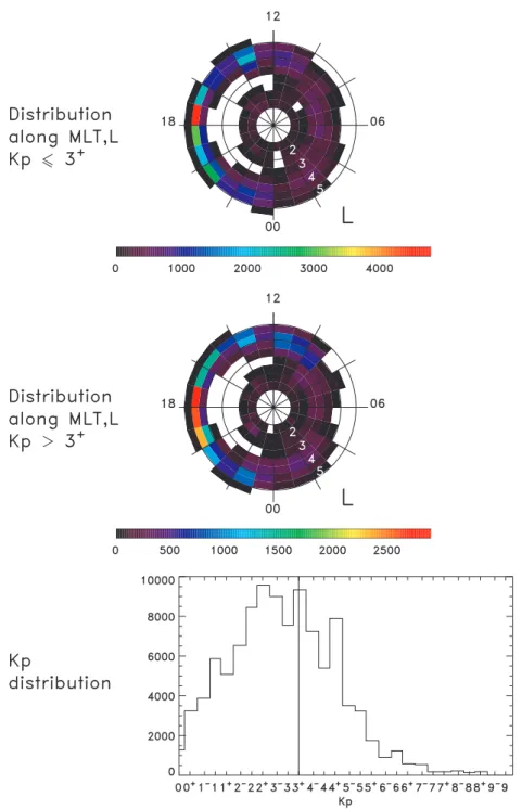
The spatial coverage of measurements during the period con-sidered is shown in Fig. 1. In order to take into account the geomagnetic activity, the database has been split into two parts, according to Kpindex values with a threshold defined at 3+. The two polar plots display the number of measured spectra with regards to the L and MLT values: for weak ge-omagnetic activity (Kp ≤ 3+) and for strong geomagnetic activity (Kp >3+). The resolution is a 0.5 unit in L-values and 1 h in MLT values. If one considers that above 30 events (i.e. practically, from the pink colour of the code) the compu-tation of a statistical quantity makes sense (Bendat and
Pier-sol, 1971), one observes that statistical analyses are possible in the major part of the L/MLT domain. However, there are important gaps: on the afternoon side, between L = 2 and 4, and on the morning side, above L = 3 to 4.
The magnetic activity recorded on the ground during this period is shown on the bottom panel of Fig. 1. The dis-tribution of Kp index peaks around 2+ and has a long tail. Considering a large Kpindex database (from 1970 to 1995, source: World Data Center C1 for Geomagnetism, Danish Meteorological Institute, Denmark), one can show that this distribution shapes like the one expected during periods of intense solar activity.
2.4 Observed emissions
The time and frequency resolutions of the DE-1 data does not allow one to make unambiguous identifications of the observed emissions. However, spectral properties recalled in the Introduction may be used in order to have a rough idea of the type of emissions. Considering that from L = 2 to
L = 5 the electron gyrofrequency at the equator runs from
∼110 kHz to 6 kHz, one may consider that:
– emissions detected between 10 and 30 kHz are
gener-ated by ground-based VLF transmitter waves,
– emissions detected between 3 kHz and 10 kHz are
cho-rus events,
– for L ≤ 2.7, emissions in between 1 kHz and 3 kHz
are plasmaspheric hiss emissions (the lowest cut-off fre-quency, at 0.1 fce, is above 3 kHz),
– however, for L > 2.7 there is no way to make the
dis-tinction between plasmaspheric hiss emissions and cho-rus events,
– emissions in the frequency range 100 Hz–1 kHz are
mainly plasmaspheric hiss,
– there is an exception for equatorial emissions below
∼250 Hz which are mainly MSW or ICW, with a non-null probability that ICW will be left-handed polarized waves.
No identification procedure has been forecast for waves above 30 kHz, whose contribution to interactions with elec-trons in the radiation belts is supposed to be negligible.
3 Variations of averaged amplitude spectra with regards to the geophysical parameters
For the sake of convenience, statistics have been made on the power spectral density of the magnetic wave field S(f ) (with
S(f ) = SBz(f ), the auto-power spectra of the parallel field component), then transformed in amplitude spectrum via the relation A(f ) =√S(f ).
Fig. 1. From top to bottom: Distribution of measurements as a function of MLT for low (top panel) and high (middle panel) magnetic activity,
and distribution of the Kpindex during the analyzed period (bottom panel).
3.1 Estimation of averaged amplitude spectra 3.1.1 Instrumental noise
A grid has been defined with a resolution of 1 h in MLT and 1 unit in L-values. For each data-base (weak and strong ac-tivity) and each cell, we define the minimum power spectrum (Smin(f, L,MLT, Kp)) of the magnetic wave field measured by the Plasma Wave Instrument on board DE-1. Taking into account the fact that the instrumental noise is independent of the satellite position, we consider that the power spectrum
of the instrumental noise at a given frequency is the me-dian value of the Sminvalues estimated in all the cells, which
writes: Snoise(f ) =MEDIAN{Smin(f, L,MLT, Kp)}. This may lead to a rejection of weak natural emissions just above the noise. There is one exception for VLF transmitters at about 14 Hz where waves are always present. Therefore, the instrumental noise at this frequency cannot be estimated. Al-though, a smooth increase in time of the instrumental noise level has been observed, using a period of time when no emission is observed, it has been checked that the median
value of Smingives a very good estimation of the real
instru-mental noise.
3.1.2 Derivation of statistical quantities
To characterize the wave activity and to build a model, we need to estimate a representative amplitude spectrum as a function of the spacecraft location and of the magnetic ac-tivity. This is done by averaging all the amplitude spectra with regards to the grid defined previously. In parallel, for each frequency, one can build a probability distribution func-tion (p.d.f.) of the power spectrum of the observed magnetic wave fields. The instrumental noise is included.
To remove small fluctuations in each cell, we first compute an average value (sv(f )) over a window that has a length of √
N points, where N is the number of points in the cell
sv(f ) = 1 √ N j · √ N + √ N −1 X k=j ·√N S(f ). (1)
Then, a mean value (Sv(f )) is computed over the √ N de-terminations of sv Sv(f ) = 1 √ N √ N −1 X j =0 sv(f ). (2) 3.1.3 Confidence interval
Given that the p.d.f. is generally non-Gaussian, we estimate the equivalent of the confidence interval using the following procedure. We estimate the standard deviation of S(f ) as follows: σ (f ) = v u u u t 1 √ N −1 √ N −1 X j =0 (sv(f ) − Sv(f ))2. (3)
Then, we estimate the confidence interval in the Gaussian approximation. In that case, there is a probability of 70% to have any S(f ) in between Sv(f ) ± σ. In our case (non-Gaussian), we just check that this confidence interval has a physical sense by computing the number of data which are included in it. If more than 50% of the data are in those limits, we consider that this Gaussian confidence level still makes sense.
3.2 Main characteristics of the averaged amplitude spectra 3.2.1 About estimated confidence intervals
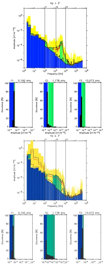
Figure 2 shows two examples of mean amplitude spec-trum (Av(f ) =
√
Sv(f ), in nT.Hz−1/2), recorded near the plasmapause between 22:00 and 23:00 MLT for weak and strong magnetic activity, and the amplitude p.d.f. taken at three frequencies 0.1, 1.178 and 10.073 kHz.
For each amplitude spectrum, the following are indicated: the instrumental noise level Anoise(f )(blue bars), the Av(f ) averaged values (red lines), the Gaussian confidence intervals
(upper and lower black lines), the intervals in which the gaus-sian confidence intervals make sense (green bars) and the ex-treme values recorded during the spacecraft mission (yellow bars). For each selected frequency, the amplitude p.d.f. is displayed with black bars, together with the computed aver-age value Av(fi)(vertical red line), the Gaussian confidence interval (green bars, shown even if it does not make sense) and the instrumental noise (blue bars).
Let us first examine the top panels without taking into ac-count the emissions above 30 kHz, whose contribution to in-teractions with electrons in the equatorial regions are sup-posed to be negligible. The estimation of a confidence in-terval makes sense in a few frequency ranges (the frequency domains coloured in green). The broadest domain (800 Hz– 3 kHz) corresponds to frequencies where plasmaspheric hiss and chorus may be detected. To understand the size of the confidence interval, one may examine the probability of oc-currence at 1.178 kHz. It is characterized by a strong peak, due to the instrumental noise, then by a continuous decrease towards the highest amplitudes. Amplitudes above the mean value are observed only in 5% of the cases. In the other fre-quency domains, the situation is still worse. The data are dominated by the instrumental noise and natural emissions are observed in a few percentage of cases. As an example, around 100 Hz, emissions seen with an amplitude of the or-der of ∼ 10−12 nT.Hz−1/2 correspond only to 0.1% of the data.
Similar conclusions may be drawn from the examples given in the bottom panels. Confidence intervals make sense over most of the frequency band of the plasmaspheric emis-sions and in several frequency bands of chorus events. Al-though the corresponding probability of occurrence has not been given for those frequencies, one notes that the largest confidence intervals, and so the largest variations, are ob-tained around 3.5 and 4.5 kHz, in the chorus band.
Examples in Fig. 3 show more narrow and so more useful confidence intervals between 500 Hz and 4 kHz for L-values below 4. The top panels show that emissions observed in this frequency band, for 2 < L < 3 and 9 < MLT < 10, are very stable, regardless of the level of geomagnetic activity. It would be interesting to check this stability for all MLT values.
3.2.2 About the amplitudes
Even if the waves with a strong amplitude represent a small percentage of data, they are of primary importance in our study, since they are the ones which have the stronger effects on the acceleration and the precipitation of electrons. Fig-ure 3 shows the following featFig-ures:
– except for the emissions observed in the band 500 Hz–
4 kHz at L-values below 3, the wave amplitudes are much greater for Kp > 3+ than for Kp ≤ 3+; this is particularly true for frequencies below 100 Hz;
– Regardless of the L-values considered and independent
Fig. 2. Wide panels: Averaged amplitude spectrum (red lines) with the instrumental noise level (blue bars), the Gaussian confidence intervals
(upper and lower black lines), the intervals in which the Gaussian confidence intervals make sense (green bars) and the extreme values recorded during the spacecraft mission (yellow bars). Small panels (three frequencies): Amplitude p.d.f. (black bars) with the computed average value (vertical red line), the Gaussian confidence interval (green bars, shown even if it does not make sense) and the instrumental noise (blue bars).
Fig. 3. Averaged amplitude spectra (red lines) in various geophysical conditions with: the instrumental noise level (blue bars), the Gaussian
confidence intervals (upper and lower black lines), the intervals in which the Gaussian confidence intervals make sense (green bars) and the extreme values recorded during the spacecraft mission (yellow bars).
are found: in the morning sector, for frequencies be-low 100 Hz, and in the afternoon sector for frequencies above.
One must be very cautious to extrapolate such charac-teristics at the vicinity of the plasmapause. As an exam-ple, coming back to Fig. 2, one observes that waves at fre-quencies below 100 Hz seem to have stronger amplitudes for
Kp≤3+than for Kp>3+. However, this is due to the rela-tive position of the satellite with regards to the plasmapause. During periods of weak geomagnetic activity, a satellite at 4 < L < 5 is within the plasmasphere. But, during peri-ods of strong geomagnetic activity, at the same location, a satellite may be outside the plasmasphere. Such an interpre-tation is supported by the bottom spectrum of Fig. 2 where the strong increase in the amplitude at ∼ 8 kHz seems to be
due to chorus events observed out of the plasmasphere. 3.3 Variation of the wave amplitudes in L and Mlat 3.3.1 Magnetic latitude
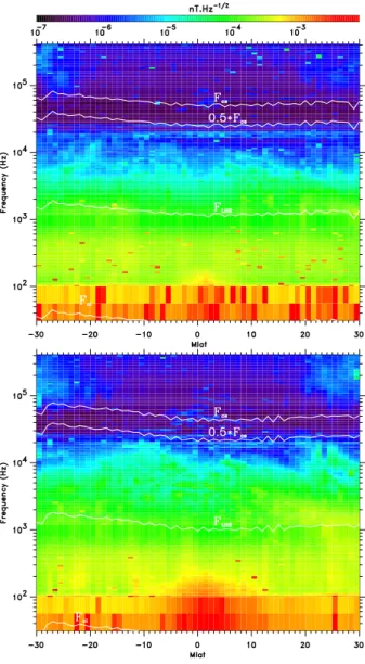
In order to examine the variations of the wave amplitude with regards to the magnetic latitude we proceed as follows. The data are averaged over the full range of MLT and L-values. Magnetic latitudes are ordered from −30◦to +30◦, with a resolution of 1◦. The results are presented in Fig. 4 for weak and strong geomagnetic activities (upper and lower panels, respectively) in colour-coded spectrograms. Characteristic frequencies (derived from magnetometer measurements, and averaged over MLT and L) are superimposed. The following are represented: fce, 0.5 fce, fLHRand fH+.
Examining the two panels of Fig. 4, from the highest to the lowest frequencies, one observes:
– weak frequency line emissions around 20 kHz,
associ-ated with ground-based VLF transmitters,
– emissions at and above the lower hybrid resonance
fre-quency fLHR, with maximum amplitudes off the
equa-tor: the stable band around fLHRcould be due to hiss
emissions, the band off the equator, which varies in fre-quency and has a much stronger amplitude during ge-omagnetically active periods, is due mainly to chorus events,
– a band of stable emissions between 200 and 800 Hz,
which can be attributed to plasmaspheric hiss emissions,
– strong equatorial emissions (probably MSW) which are
very sensitive to the geomagnetic activity: for low Kp values, higher cut off frequency at ∼ 150 Hz and Mlat values between −2◦and +5◦; for high K
pvalues, higher cut off frequency at ∼ 250 Hz and Mlat values between
−8◦and +13◦,
– the instrumental noise masks emissions (ICW) which
are probably present below fH+. 3.3.2 L-values
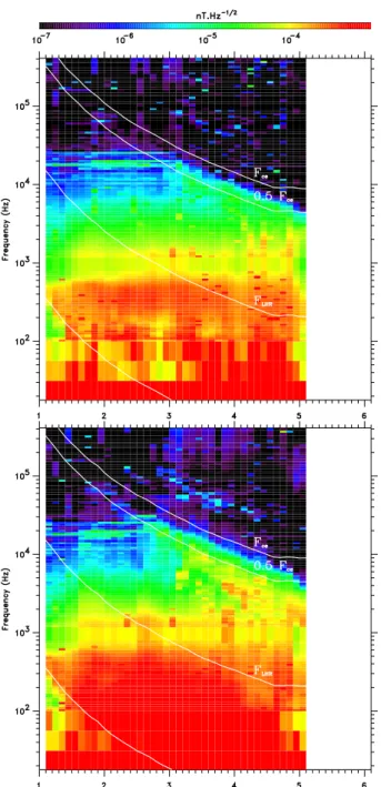
Figure 5 shows the variation in L of the average spectra for waves recorded around the equator (|Mlat| < 15◦), for weak (upper panel) and strong (lower panel) magnetic ac-tivity. Spectra are sampled by steps of 0.1 in L-values, and averaged over latitudes and magnetic local times. The main features are as follows:
– waves associated with VLF transmitters appear very
clearly in the frequency band 10–25 kHz. They are ob-served mainly at L < 3, where their frequency is well below the electron gyrofrequency (fce). At higher L-values, a clear cutoff appears around 0.5 fce. As ex-pected, there is no emission above fce,
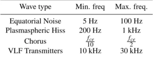
Table 1. Frequency bands defined to estimate wave occurrence
Wave type Min. freq Max. freq. Equatorial Noise 5 Hz 100 Hz Plasmaspheric Hiss 200 Hz 1 kHz Chorus fce 10 fce 2 VLF Transmitters 10 kHz 30 kHz
– following the variation in L of the electron
gyrofre-quency, a band of emissions is seen between ∼ 0.1 and 0.8 fce, with amplitudes reaching 10−3nT.Hz−1/2; they are chorus events, much more intense during periods of strong geomagnetic activity,
– the lower panel shows a persistent narrow band of hiss
emission at 1.2 kHz (may be contaminated by instru-mental noise) with an amplitude (≈ 10−4nT.Hz−1/2) slightly increasing with the geomagnetic activity,
– there is a persistent emission from approximately
100 Hz to 3 kHz, with maximum amplitudes of the order of 10−3nT.Hz−1/2in the band 200–800 Hz; the emis-sion (plasmaspheric hiss) is affected marginally by an increase in the geomagnetic activity,
– observed mainly during periods of strong
geomag-netic activities (see the bottom panel), a broadband emission is present from frequencies below fH+ to frequencies below fLHR; the amplitudes which reach
10−2nT.Hz−1/2 are maximum for 3.5 < L < 5; in agreement with Fig. 4, the band of emission seems dom-inated by MSW waves; ICW emissions are probably present below fH+.
4 Occurrence of each class of emission
In order to make comparisons with databases from other satellites, the occurrence of each type of emission has been estimated in L/MLT domains.
4.1 Definition
According to the remarks made in Sect. 2.4, an automatic classification is possible from the criteria given in Table 1. In so doing: (i) one restricts the plasmaspheric hiss to the frequency band originally defined by Thorne et al. (1973), (ii) one limits the confusion between hiss and chorus around 0.1 fce, without removing it completely, (iii) one does not take into account the upper-band of chorus, which is anyway much less intense than the lower one (see Figs. 4 and 5).
Practically, all spectra are spatially localised in a grid de-fined in the (MLT, L) coordinates system that have a spatial resolution of 1 h MLT and 0.5 in L-values. In a given cell, a particular wave is defined to be observed when the spectrum amplitude is more than 10 dB above the noise level, at least at
Fig. 4. Variation in Mlat values of the amplitude spectra averaged over L-values running from 1 to 5.5. The top panel corresponds to spectra
recorded during periods of weak geomagnetic activity and the bottom panel to spectra recorded during periods of strong geomagnetic activity.
one frequency inside the frequency band considered. There-fore, the occurrence is the percentage of time this particular wave has been observed, during the whole mission in a given spatial location.
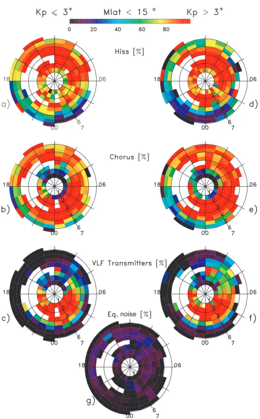
4.2 Probability of observing each type of emission in
L/MLT domains
Figure 6 shows the color-coded probability of observing (from top to bottom) the plasmaspheric hiss, the chorus, the VLF transmitters and the equatorial noise as a function of the local time and L. Left and right panels give the occurrence when using the weak and strong magnetic activity databases, respectively. Since the probability of observing the equato-rial noise is very small (and statistically non-significant), it is only given for all Kp conditions. In general, these panels
suffer from a lack of points in the databases. Therefore, only their general tendency can be given.
Regardless of the geomagnetic activity, the plasmaspheric hiss is observed mainly on the dayside. However, the exten-sions in L-values depends on the Kpvalues. For Kp ≤ 3+, the emission extends from L = 1.5 to 5.5 at noon, whereas it concentrates around L = 3 at midnight. For Kp >3+, the extension is limited to L = 1.5 to 4.5 at noon, whereas it runs from L = 1.5 to 3 at midnight. According to the fact that the colour code gives the probability of finding an emission with a signal to noise ratio greater than 10 dB, one concludes that we are consistent with Russell et al. (1969), who pointed out a decrease in amplitude (not in occurrence) in the nightside, and with Smith et al. (1974), who found an increase in am-plitude in the same region during intense magnetic activities. The data gap in the dusk sector, the lack of data above
Fig. 5. Variation in L-values of the amplitude spectra averaged over
Mlat values running from −15◦to +15◦. The lower panel cor-responds to spectra recorded during periods of weak geomagnetic activity and the bottom panel to spectra recorded during periods of strong geomagnetic activity.
L = 5.5 and the remaining ambiguity with plasmaspheric hiss at the lowest frequencies prevent one from pointing out all the characteristics of the chorus events. However, one ob-serves: (i) a probability that increases above L = 2, (ii) an extension in L-values which goes up to L = 5.5 for records made at noon during periods of strong geomagnetic activ-ities, (iii) a tendency for a higher probability on the dawn side, particularly for high Kpvalues.
Most of the VLF transmitters emission are observed in the
nightside, at L ≤ 3.5. This limit corresponds to the cutoff at fce. This result is fully consistent with the conclusions given by Imhof et al. (1984). Another maximum is found at noon around L = 2.5 in a very small area, which increases a bit in size with the magnetic activity. We suspect that this particular observation is not real, since the number of points that defines the occurrence in these cells is rather low for both databases (see Fig. 1).
Even when merging observations made during weak and strong geomagnetic activities, the probability defined for the equatorial emissions is very weak. This seems to be due to our selection criterion (signal to noise ratio greater than 10 dB), which is too strict for emissions whose amplitudes are often just above the instrumental noise. Although the statistics are insufficient to draw any conclusions, it seems that the distribution of the events in MLT is rather isotropic, as suggested by Kasahara et al. (1992, 1994).
5 The model
5.1 Definitions
An analytical expression Ai of the amplitude spectral density has been derived for each type of emission. It is written in the form:
Ai =ai(f,Mlat, MLT) · 9i(Mlat, MLT, L, Kp) · Ci(f ).(4) Simple mathematical functions have been used to repre-sent averaged DE-1 data. The ai(f )function has been con-structed from the mean value of all DE-1 amplitude spec-tra of the it h type of mission for given Mlat and L-values. The 9i(Mlat, MLT, L, Kp) function has been established from large-scale variations observed in Fig. 4 (dependence in Mlat), Fig. 5 (dependence in L) and Fig. 6 (occurrence in the L/MLT domain). The Ci(f )function is more objective, since it introduces cutoff frequencies for each type of emis-sion, with the proton gyrofrequency fH+ being computed from the onboard magnetometer data.
The wave model A is the sum of the Aimodels:
A =X
i
Ai. (5)
One cannot expect that it reproduces exactly a measured am-plitude spectral density since first, all the emissions do not necessarily appear all together, and second, it has been con-structed from averaged data.
5.2 Main characteristics of the model constructed for each emission
The VLF transmitters waves are observed only on the night-side, where propagation conditions from the Earth to the plasmasphere are favorable (Imhof et al., 1984). The mod-elled transmitters are those given by Parrot (1990). On aver-age, the amplitude of each transmitter is chosen to be of the order of 10−6nT.Hz−1/2. As seen by the PWI instrument, this contribution has a upper cutoff at 0.8 fce.
noise
Fig. 6. Probability of observing types of emission for weak (left panels) and strong magnetic activity (right panels). From top to bottom: (a)
and (d) Plasmaspheric hiss, (b) and (e) Chorus, (c) and (f) VLF transmitters and (g) Equatorial noise.
As observed in Fig. 5, the frequency of the maximum am-plitude of chorus events follows a law proportional to 0.35
fce. The amplitude is of the order of 10−5nT.Hz−1/2 and increases with L (Burtis and Helliwell, 1975). We have taken into account the occurrence described by Tsurutani and Smith (1977), Koons and Roeder (1990) and Sazhin and
Hayakawa (1992), despite that the data gap on the afternoon sector did not allow its quantification.
In agreement with PWI observations, the plasmaspheric hiss has two components. The first one is centered around 300 Hz and has a maximum amplitude of 1.5 × 10⁻³nT.Hz−1/2, whereas the second component has a
maxi-mum amplitude of 3 ×10⁻⁴nT.Hz−1/2at 1 kHz. These
emis-sions are observed in the dayside plasmasphere, but also in the nightside when the magnetic activity is high.
Following Perraut et al. (1982), the MSW must be repre-sented by a function having a maximum amplitude (a few nT.Hz−1/2) at fH+ and a decreasing law for higher har-monics. However, disagreements between occurrence stud-ies made on GEOS-1 (Perraut et al., 1982) and AKEBONO (Kasahara et al., 1992; 1994), plus the lack of data on DE-1 (see Fig. 6) prevents us from constructing a reliable model. The only clear feature is the extension in the frequency do-main and in the L-values, when one moves from periods of weak geomagnetic activity to periods of strong geomagnetic activity. But in this first version of the model, we did not take into account such a Kp dependence. In this database, averaged amplitude spectra seem to increase in the MSW fre-quency band around 21:00 MLT and 03:00 MLT. Despite the fact that this feature is not statistically significant (compared to amplitudes observed in other MLT, L sectors), the model reproduces this behaviour.
Observed data do not allow one to model ICW. Few es-timations of the sense of polarization have been published. Presently, the best thing to do is probably to make the hy-pothesis that ICW are right-handed polarized or left-handed polarized. In this paper, we have chosen to include not ICW waves (left-handed polarization hypothesis). Therefore, the lower cutoff frequency is at fH+.
5.3 Results
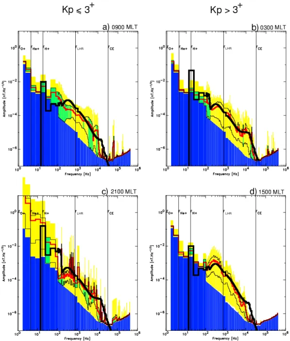
Figure 7 shows examples of comparisons between the ampli-tude averaged spectral densities (red lines) observed by PWI and the modelled ones (heavy solid black line). The instru-mental noise (blue bars) and the maximum amplitudes (yel-low bars) have been superimposed on the spectra. For the sake of convenience, characteristic frequencies have been in-dicated (the lower hybrid frequency fLHR and various
gy-rofrequencies: fce, fH+, fHe+, fO+, vertical black lines). Observations are taken at L = 3 and at 09:00, 03:00, 21:00 and 15:00 MLT from left to right and top to bottom. The
Kpindex is below and above 3+on the left and right panels, respectively.
The modelled spectra have been estimated from 2400 points logarithmically-spaced from 1 Hz to 1 MHz. To com-pare with DE-1 data, we have reduced these spectra to repro-duce the PWI spectral resolution (average over sensor band-widths).
The way in which the model fits the data relative to each type of emission may be summarized as follows:
– the model for the emissions generated by the VLF
trans-mitters gives orders of magnitude only; more precise comparisons are impossible, since the DE-1 data do not allow to identify each transmitter frequency, whereas the transmitter frequencies have been introduced in the model,
– the modelling of the hiss and chorus emissions is quite
correct in all cases; however, the amplitude of plasma-spheric emissions is slightly overestimated during peri-ods of weak geomagnetic activity,
– despite the strong uncertainties we have for equatorial
emissions, the fit is not too bad for the MSW. There is an exception for the observations at 09:00 MLT, where the amplitudes are clearly underestimated between 30– 100 Hz. In this particular case, this disagreement can be reduced by increasing the high order harmonic ampli-tudes, or by increasing their number.
When the magnetic activity increases, at 03:00 MLT, the agreement between the model and the observed spectrum is very good. The only disagreement comes from the equato-rial noise and more precisely, at frequencies close to fH+. By opposition, the contribution from the fH+ harmonics re-produces well the observation (above 35 Hz). We can explain this discrepancy by the fact that we take the MSW fundamen-tal frequency at fH+, which is not always the case (Perraut et al., 1982).
5.4 Comparison with OGO-5 and GEOS data
In order to qualify our wave model, we have taken the geo-physical parameters of observations made on the GEOS-1 (Solomon and Cornilleau-Wehrlin, GEOS-1988) and OGO-5 (Thorne et al., 1973) satellites, then we have compared the predicted amplitude spectral densities to the measured ones. The results are displayed in Fig. 8. As in Fig. 5, the pre-dicted spectra are represented by heavy black lines, and the measured spectra by blue lines. The measured DE-1 spectra are represented by yellow bars.
Let us first consider a GEOS-1 spectrum (left panel). It is extracted from the right panel of Fig. 4 of Solomon and Cornilleau-Wehrlin (1988). The observation was made on 8 March 1978 at about 03:40 UT (Jones, 1978; S300 Experi-menters, 1979), when the satellite was located at 04:00 MLT,
L = 4.7 near the magnetic equator (Mlat = 10◦), in a time period of very low activity (Kp = 1+ after 6 days of Kp values less than 3+). Information about the way to estimate the spectrum can be found in Jones (1978) and S300 Exper-imenters (1979). Although not discussed by the authors, the peaks around 500 Hz and 1.8 kHz can be attributed to plas-maspheric hiss and chorus emissions, respectively. The fact that the amplitude values are much larger than the mean val-ues detected by DE-1 is not surprising for published data. Authors often use the best cases to illustrate their papers. In such a situation, it is not surprising that the predicted spec-trum underestimates the measured ones. The underestima-tion is a factor of 2 for the plasmaspheric hiss part, which was shown to be quite stable, and a factor of 10 for the cho-rus part, which may be more variable. One may consider that the wave model provides a satisfactory prediction of the amplitude spectrum.
An OGO-5 spectrum is displayed on the right panel of Fig. 8. It is extracted from the Fig. 2 of Thorne et al.
Fig. 7. Comparison between modelled (heavy black line) and observed (red lines) averaged amplitude spectra at L = 3 and (a) 09:00 MLT, (b) 03:00 MLT, (c) 21:00 MLT and (d) 15:00 MLT. The magnetic activity is weak on left panels and strong on right panels. The instrumental
noise (blue bars) and the maximum amplitudes (yellow bars) have been superimposed on the spectra.
(1973). The observation was made on 4 April 1968, around 10:00 UT, at a time of moderate to weak geomagnetic ac-tivity. At this time, the spacecraft was at L ∼ 3, around 12:00 MLT, at a magnetic latitude smaller than 15◦. The spectrum was given as an example of plasmaspheric hiss by the authors. The predicted spectrum underestimates the mea-sured spectrum by a factor of 2.5. In a sense, this result is satisfactory, since it is difficult to improve when comparing an instantaneous spectrum to an average one. However, the fact that the values obtained from the OGO-5 data are higher than the maximum values never obtained during 3 years of DE-1 observation makes one question either the respective
calibration of the magnetic sensors or the stability of the emission over a long time period (here, 15 years). Despite the numerous observations made in the magnetosphere, the extreme values are unknown.
6 Conclusions
A statistical study of 3 years of DE-1 data has been per-formed with the aim of elaborating a model of the waves that can interact with electrons in the equatorial regions of the plasmasphere. Since the time and frequency resolutions
Fig. 8. Amplitude spectra recorded (blue line) on board (a) GEOS-1 and (b) OGO-5 compared with the averaged amplitude spectra modelled
(heavy black line) for similar geophysical conditions. The measured spectra recorded by DE-1 are shown with yellow bars.
are insufficient to make an unambiguous identification of the type of emissions involved, the criteria based on frequency values have been used to make the distinction between: VLF transmitter emissions, plasmaspheric hiss emissions, chorus emissions, and equatorial emissions below ∼ 200 Hz. It has been validated that the class of emissions, so defined, repro-duces most of the characteristics pointed out by previous au-thors.
Distributions in L, Mlat and MLT values of the averaged amplitude spectral densities of the wave magnetic fields have shown that the emissions which are the most sensitive to vari-ations in geomagnetic activity were first the equatorial emis-sions below ∼ 200 Hz, then the chorus. If the sensitivity of the chorus emissions to variations in geomagnetic activity was known for a long time (see Meredith et al., 2001, and references therein), then it does not seem that the effect on the equatorial emissions was reported before. Confidence in-tervals estimated for the averaged spectral densities allowed one to confirm that statement. The narrowest confidence in-tervals are obtained for plasmaspheric emissions whose am-plitude spectral densities are rather stable during the three years of DE-1 observations. Broader confidence intervals, i.e. larger variations, are obtained for chorus and equatorial emissions.
Analytical expressions of the amplitude spectral densities of the wave magnetic fields have been derived for each type of emissions from DE-1 amplitude spectral densities aver-aged either on all L-values or on all MLT values. The wave model A(f, L, Mlat, MLT, Kp)has been constructed from the sum of these analytical expressions. It is given in nT.Hz−1/2. It has been first tested on DE-1 amplitude
spec-tral densities averaged over limited sectors of the L/MLT do-main. The main results are as follows:
– the wave model provides values of the amplitudes of
the VLF transmitter frequencies which look reasonable with regards to the DE-1 data in a given sector, but the frequency resolution of the full set of DE-1 data is insuf-ficient both to elaborate on an accurate model and then to test its performances,
– although a slight overestimation of the amplitudes is
ob-served, particularly for weak geomagnetic activity, the wave model provides rather good predictions for the plasmaspheric hiss and chorus frequency bands,
– predictions are not always reliable for equatorial
emis-sions below ∼ 200 Hz: first, the variability in the MSW waves requires much more data to elaborate on a robust model; second, DE-1 data do not allow one to model ICW waves.
The wave model derived from the DE-1 data has also been tested on amplitude spectral densities estimated from OGO-5 and GEOS-1 data. The prediction underestimated the es-timated values by a factor of 2 to 2.5 for plasmaspheric hiss emissions and by a factor of 10 for chorus emissions. This can be considered as correct for comparisons between instan-taneous spectra and average spectra, with the spectra of the chorus events having obviously larger confidence intervals than the spectra of hiss.
Now, in several occasions, the lack of data has been pointed out. Data gaps prevented us from quantifing asym-metry between observations made in the morning and in the afternoon. Statistics on the MSW waves were much too weak. Full characterizations of ICW waves are needed. Data outside L = 6 are needed (Horne and Thorne, 1998). Am-plitude values observed on OGO-5 show that 3 years of data are insufficient to estimate the averaged and extreme values of the amplitudes of natural emissions.
Obviously, more data are required to improve the wave model. Among the supplementary observations to be made, priorities may be given to:
– measurements of one magnetic wave field component
above ∼ 200 Hz over several years (if possible, a so-lar cycle), to complete the databases available presently and to point out the variation of the amplitude spectral density A(f ) as a function of the geomagnetic activity.
– measurements of the three magnetic components below
∼200 Hz, to point out the right-handed polarized waves below the local proton gyrofrequency, and to identify the waves that potentially precipitate the highest en-ergy electrons. In the quasi-absence of relevant data out of L = 6, the modelled amplitude spectrum be-low the local proton gyrofrequency is supposed to be ei-ther the spectrum of left-handed polarized waves, which means that there is no interaction with trapped electrons above ∼ 1 MeV, or the spectrum of right-handed polar-ized waves, which means that there is a maximum inter-action with trapped electrons above ∼ 1 MeV;
– measurements of the three magnetic components in a
wider frequency range, to provide a model of wave nor-mal directions that control the growth rate in the equa-torial region.
Acknowledgements. The authors are most grateful to the referees
for excellent remarks and suggestions. They thank their colleague X. Valli`eres for his help in the manuscript edition. The work has been supported by contract CEA/DAM. The Kp index data have
been provided by the World Data Center C1 for Geomagnetism. Topical Editor G. Chanteur thanks A. Smith and another referee for their help in evaluating this paper.
References
Abel, B. and Thorne, R.: Electron scattering loss in Earth’s in-ner magnetosphere 1. dominant physical processes, J. Geophys. Res., 103, 2385, 1998a.
Abel, B. and Thorne, R.: Electron scattering loss in Earth’s in-ner magnetosphere 2. sensivity to model parameters, J. Geophys. Res., 103, 2397, 1998b.
Baker, D. N., Belian, R. D., Highie, P. R., Klebesadel, R. W., and Blake, J. B.: Deep dielectric charging effects due to high energy electrons in earth’s outer magnetosphere, J. Electrostat., 20, 3, 1987.
Baker, D. N., Kaneckal, S., Blake, J. B., Klecker, B., and Rostoker, G.: Satellite anomalies linked to electron increase in the magne-tosphere, EOS, 75, 401, 1994.
Bendat, J. and Piersol, A.: Random data : analysis and measure-ment procedures, Wiley-Interscience, New-York, 1971. Burtis, W. and Helliwell, R.: Magnetospheric chorus: Amplitude
and growth rate, J. Geophys. Res., 80, 3265, 1975.
Cornilleau-Wehrlin, N., Gendrin, R., Lefeuvre, F., Parrot, M., Grard-R, R., Jones, D., Bahnsen, A., Ungstrup, E., and Gib-bons, W.: VLF electromagnetic waves observed onboard GEOS-1, Space Sci. Rev., 22, 37GEOS-1, 1978.
Cornilleau-Wehrlin, N., Solomon, J., Korth, A., and Kremser, G.: Generation mechanisms of plasmaspheric ELF/VLF hiss: a sta-tistical study from GEOS-1 data, J. Geophys. Res., 98, 21 471, 1993.
Gurnett, D. and Inan, U.: Plasma wave observation with the Dy-namic Explorer-1 spacecraft, Rev. Geophys., 26, 285, 1988. Hattori, K., Hayakawa, M., Lagoutte, D., Parrot, M., and
Lefeu-vre, F.: Further evidence of triggering chorus emissions from wavelets in the hiss, Planet. Space Sci., 19, 1465, 1991. Hayakawa, M. and Sazhin, S.: Mid-latitude hiss and plasmaspheric
hiss: A review, Planet. Space Sci., 40, 1325, 1992.
Horne, R. and Thorne, R.: Potential waves for relativistic electron scattering and stochastic acceleration during magnetic storms, Geophys. Res. Lett., 25, 3011, 1998.
Imhof, W., Gaines, E., and Reagan, J.: Evidence for the resonance precipitation of energetic electrons from the slot region of the radiation belts, J. Geophys. Res., 79, 3141, 1974.
Imhof, W., Anderson, R., Reagan, J., and Gaines, E.: The signifi-cance of VLF transmitters in the precipitation of inner belt elec-trons, J. Geophys. Res., 86, 11 225, 1981.
Imhof, W. L., Reagan, J., Gaines, E., and Datlowe, D.: The L shell region of importance for waves emitted at ground level as a loss mechanism for trapped electron > 68 keV, J. Geophys. Res., 89, 10 827, 1984.
Inan, U.: Gyroresonant pitch angle scattering by coherent and inco-herent whistler mode waves in the magnetosphere, J. Geophys. Res., 92, 127, 1987.
Inan, U. and Helliwell, R.: DE-1 observations of VLF transmit-ter signals and wave-particle intransmit-teractions in the magnetosphere, Geophys. Res. Lett., 9, 917, 1982.
Jones, D.: Introduction to the S-300 wave experiment on board GEOS, Space Sci. Rev., 22, 327, 1978.
Kasahara, Y., Sawada, A., Yamamoto, M., Kimura, I., Kokubun, S., and Haayashi, K.: Ion cyclotron emissions observed by the satellite Akebono in the vicinity of the magnetic equator, Radio Sci., 27, 347, 1992.
Kasahara, Y., Kenmochi, H., and Kimura, I.: Propagation charac-teristics of the ELF emissions observed by the satellite Akebono in the magnetic equatorial region, Radio Sci., 4, 751, 1994. Koons, H. and Roeder, J.: A survey of equatorial magnetospheric
wave activity between 5 and 8 RE, Planet. Space Sci., 38, 1335,
1990.
Lefeuvre, F. and Parrot, M.: The use of the coherence function for the automatic recognition of chorus and hiss observed by GEOS, J. Atmos. Terr. Phys., 41, 143, 1979.
Li, X., Baker, D., Temerin, M., Cayton, T., Reeves, G., Chris-tiansen, R., Blake, J., Looper, M., Nakamura, R., and Kanekal, S.: Multisatellite observations of the outer zone electron varia-tion during the November 3-4, magnetic storm, J. Geophys. Res., 102, 14 123, 1997.
Lyons, L., Thorne, R., and Kennel, C. F.: Pitch-angle diffusion of radiation belt electrons with the plasmasphere, J. Geophys. Res., 77, 3455, 1972.
Meredith, N., Horne, R., Johnstone, A., and Anderson, R.: The tem-poral evolution of electron distributions and associated wave ac-tivity following substorm injections in the inner magnetosphere, J. Geophys. Res., 105, 12 907, 2000.
Meredith, N., Horne, R., and Anderson, R.: Substorm dependence of chorus amplitudes : implications for the acceleration of elec-trons to relativistic energies, J. Geophys. Res., 106, 13 165, 2001. Ondoh, T., Nakamura, Y., Watanabe, S., Aikyo, K., and Murakami, T.: Plasmaspheric hiss observed in the topside ionosphere at
mid-and low-latitudes, Planet. Space Sci., 41, 411, 1983.
Parady, B., Eberlein, D., Marvin, J., Taylor, W., and Cahill, L.: Plas-maspheric hiss observations in the evening and afternoon quad-rants, J. Geophys. Res., 80, 2183, 1975.
Parrot, M.: World map of ELF/VLF emissions as observed by a low orbiting satellite, Ann. Geophysicae, 8, 135, 1990.
Parrot, M. and Lefeuvre, F., Statistical study of the propagation characteristics of ELF hiss observed on GEOS-1, inside and out-side the plasmasphere, Ann. Geophysicae, 4, 363, 1986. Perraut, S., Roux, A., Robert, P., Gendrin, R., Sauvaud, J.-A.,
Bosqued, J.-M., Kremser, G., and Korth, A.: A systematic study of ULF waves above fH+ from GEOS 1 and 2 measurements
and their relationship with proton ring distributions, J. Geophys. Res., 87, 6219, 1982.
Rostoker, G., Skone, S., and Baker, D.: On the origin of relativistic electrons in the magnetosphere associated with some geomag-netic storms, Geophys. Res. Lett., 25, 3701, 1998.
Russell, C., Holzer, R., and Smith, E.: OGO 3 observations of ELF noise in the magnetosphere : 1.spatial extent and frequency of occurrence, J. Geophys. Res., 74, 755, 1969.
Russell, C., Holzer, R., and Smith, E.: OGO 3 observations of ELF noise in the magnetosphere, 2. the nature of the equatorial noise, J. Geophys. Res., 73, 755, 1970.
Russell, C., McPherron, R., and Coleman, P.: Fluctuating magnetic fields in the magnetosphere, Space Sci. Rev., 12, 810, 1972. S300 Experimenters: Measurements of electric and magnetic wave
fields and of cold plasma parameters onboard GEOS 1: Prelimi-rary results, Planet. Space Sci., 27, 317, 1979.
Sazhin, S. and Hayakawa, M.: Magnetospheric chorus emission: A review, Planet. Space Sci., 40, 681, 1992.
Shawhan, S., Gurnett, D., and Odem, D.: The plasma wave and quasi-static electric field instrument (PWI) for Dynamic
Explorer-A, Space Sci. Inst., 5, 535, 1981.
Smith, E., Frandsen, A., Tsurutani, B., Thorne, R., and Chan, K.: Plasmaspheric hiss intensity variations during magnetic storms, J. Geophys. Res., 79, 2507, 1974.
Solomon, J. and Cornilleau-Wehrlin, N.: An experimental study of ELF/VLF hiss generation in the earth’s magnetosphere, J. Geo-phys. Res., 93, 1839, 1988.
Sonwalkar, V. and Inan, U.: Wave normal direction and spectral properties of whistler mode hiss observed on the DE-1 satellite, J. Geophys. Res., 93, 7493, 1988.
Storey, L. and Lefeuvre, F.: The analysis of 6-component measure-ments of electromagnetic wave field in a magnetoplasma, 1, the direct problem, Geophys. J. R. Astron. Soc, 56, 255, 1979. Storey, L. and Lefeuvre, F.: The analysis of 6-component
measure-ments of electromagnetic wave field in a magnetoplasma, 2, the integration kernels, Geophys. J. R. Astron. Soc, 62, 173, 1980. Summers, D. and Ma, C.-Y.: A model for generating relativistic
electrons in the earth’s inner magnetosphere based on gyrores-onant wave-particle interactions, J. Geophys. Res., 105, 2625, 2000.
Summers, D., Thorne, R., and Xiao, F.: Relativistic theory of wave-particle resonant diffusion with application to electron accelera-tion in the magnetosphere, J. Geophys. Res., 103, 20 487, 1998. Thorne, R., Smith, E., Burton, R., and Holzer, R.: Plasmaspheric
hiss, J. Geophys. Res., 78, 1581, 1973.
Tsurutani, B. and Smith, E.: Postmidnight chorus: a substorm phe-nomenon, J. Geophys. Res., 79, 118, 1974.
Tsurutani, B. and Smith, E.: Two types of magnetospheric ELF chorus and their substorm dependencies, J. Geophys. Res., 82, 5112, 1977.
Vampola, A.: VLF transmission induced slot electron precipitation, Geophys. Res. Lett., 4, 569, 1977.