phase epitaxy of m-plane GaN”
Edith Perret,1, 2Dongwei Xu,1M. J. Highland,1G. B. Stephenson,1P. Zapol,1 P. H. Fuoss,1,a)A. Munkholm,3 and Carol Thompson4,b)
1)
Materials Science Division, Argonne National Laboratory, Argonne, IL 60439 USA
2)
University of Fribourg, Department of Physics and Fribourg Center for Nanomaterials, Chemin du mus´ee 3, CH-1700 Fribourg, Switzerland
3)
Munkholm Consulting, Mountain View, CA 94043 USA
4)
Department of Physics, Northern Illinois University, DeKalb IL 60115 USA (Dated: 2017 September 14)
This supplemental material contains a description of experimental conditions and methods, methods of fitting the data to obtain island spacings Sz and Sx, and a comparison of the island spacings Sz to the step-flow boundary obtained from CTR intensity oscillations.
I. EXPERIMENTAL CONDITIONS AND METHODS
Methods were substantially the same as described previously.1 Grazing-incidence x-ray surface scattering measurements2 were performed at undulator beamline 12ID-D of the Advanced Photon Source in a verti-cal flow MOVPE chamber mounted on a z-axis surface diffractometer.3,4An x-ray energy of 28.26 keV was used to penetrate the 2-mm-thick quartz walls of the chamber. The grazing angle was set to the critical angle, α = 0.09◦, to obtain maximum surface sensitivity. Diffracted x-rays were observed with a pixel array detector.5
The single-crystal GaN substrate, crystal “C” of the previous work,1 was purchased from a commercial supplier.6 The angle of the surface with respect to the (1 0 1 0) planes, determined by atomic force microscopy, was 0.4◦, giving terraces of width W = 400 ˚A between (1 0 1 0) steps, at an azimuth of 10◦ from [0 0 0 1]. To prepare a clean surface before the growth mode studies, crystals were etched in a 10% HCl solution for 5 min and a 400-˚A-thick buffer layer of GaN was grown in situ at 1250 K.
Triethylgallium (TEGa) and ammonia (NH3) were used as precursors and nitrogen as carrier gas. The to-tal chamber pressure was 267 mbar, and the toto-tal re-active gas flow was 4.7 slpm. The sample temperature was calibrated to within ±5 K for the relevant gas flow conditions using optical interferometry measurements of the thermal expansion of a standard sapphire substrate.7 For these growth studies, the NH3 flow was kept con-stant at 2.7 slpm, and the TEGa flow was used to control growth. (The NH3 flow used, 1.2 × 10⁵µmol/min, repre-sents a large oversupply, with a V/III ratio > 105. We ob-served that the growth behavior is typically independent of NH3 flow from 2.7 down to 0.01 slpm.) Growth rates were determined by the x-ray oscillation period under
a)current address: SLAC National Accelerator Laboratory, Menlo Park, CA 94025 USA
b)correspondence to: [email protected]
layer-by-layer conditions,1 and by in situ optical inter-ferometry measurements of film thickness under step-flow conditions.3Over the complete range of conditions stud-ied, we found that the growth rate was independent of temperature and proportional to the TEGa supply rate, with a growth rate of 1.0 ± 0.1˚A/s for each µmol/min of TEGa supplied. This indicates that the growth rate is limited by precursor transport rather than surface kinetics.8Extrapolation to zero TEGa supply gives a zero growth rate, which indicates that there is negligible GaN re-evaporation under the conditions studied.
II. METHOD OF FITTING TO GET ∆Lpk AND Sz
The sequence of images obtained from the area detec-tor during each growth run were first plotted in recipro-cal space coordinates. The reciprorecipro-cal lattice units used were relative to room-temperature GaN, a0 = 3.19 ˚A, c0 = 5.18 ˚A. Values of H, K, and L reciprocal space coordinates were obtained for every detector pixel using the orientation matrix determined for the sample, the spectrometer angles, and the relative angles of each pixel of the area detector with respect to its reference pixel.9 Because the CTR and the diffuse scattering from the is-lands are extended in the surface normal H direction, the images were projected onto the KL plane to analyze the in-plane diffuse scattering from the islands. FiguresS.1
andS.2show typical images before growth and after 0.5 ML of growth, respectively, plotted in the KL plane.
One can see from Fig. S.1before growth that the reso-lution function obtained for the CTR using the grazing-incidence geometry is asymmetric in the KL plane, tilted in a direction corresponding to dL/dK ≈ 5. FigureS.2
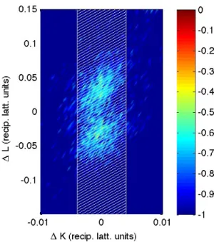
after 0.5 ML of growth is plotted using ∆K and ∆L rel-ative to the peak position before growth. The central CTR intensity at ∆K = ∆L = 0 is minimum and satel-lite peaks appear at positions ±∆Lpk around the CTR. Each of these peaks is convolved with the same tilted res-olution function. To obtain the diffuse scattering profiles I(L, t) in the L direction shown in Fig. 3 of the main pa-per, for each point we integrated the signal within each
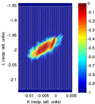
FIG. S.1. Typical diffuse intensity distribution in the KL plane around the (H 0 H 2) CTR near H = 0.5 prior to growth, showing the CTR with no diffuse scattering. Col-orbar gives log10(I). Also shown (white outlines) are the
re-gions used to integrate the intensity to produce a profile as a function of L only.
FIG. S.2. Typical diffuse intensity distribution in the KL plane around the (H 0 H 2) CTR near H = 0.5 after growth of 0.5 ML, showing the satellite diffuse scattering peaks from the islands. Colorbar gives log10(I). Also shown (white outlines)
are the regions used to integrate the intensity to produce a profile as a function of L only.
−2.10 −2.05 −2 −1.95 −1.9 −1.85 0.5 1 1.5 2 2.5 3
L (recip. latt. units)
Intensity
Data Sum Peak Bkgd
FIG. S.3. Typical diffuse intensity distributions around the CTR in the L direction prior to growth, showing the CTR with no diffuse scattering. Also shown are fits to extract the peak position, shape, and background.
of the white parallelograms shown in Figs. S.1 andS.2, which were aligned with the resolution function to pre-serve highest resolution in L. We used integration regions of width 0.008 r.l.u. in L over a range ∆K = ±0.004. A typical sequence of these profiles as a function of time during growth is shown in Fig. 2 of the main paper.
The peak position ∆Lpk at 0.5 ML coverage was ex-tracted for each growth run by fitting the profile for times near the first minimum in the CTR intensity. The first step in this process was to fit the profile prior to growth to obtain the background and the position and width of the initial CTR. The background was obtained by fitting a cubic polynomial to the tails on each side of the cen-tral peak. A Gaussian peak shape was found to fit well the background-subtracted CTR, as shown in Fig. S.3. The initial peak position, used to set the zero of ∆K and ∆L, is slightly displaced from integer values. This accounts for the temperature dependence of the lattice parameters, and any small misalignments of the crystal orientation matrix arising from temperature cycling. The background obtained from the pre-growth scattering was subtracted from all profiles in the time sequence. The remaining signal profile at the time corresponding to 0.5 ML was fit using a pair of identical Lorentzians displaced equally on opposite sides of the initial CTR position, as well as a central Gaussian peak with the same position and width as the initial CTR peak. The double Loren-ztian shape was found to work well for the diffuse scat-tering; it overestimates the tails, but fits well near the peak where it matters. To reduce the number of fit pa-rameters, the width of the Lorentzians was forced to be proportional to their displacement, with a fixed ratio of 1.75 set by the average of the (reasonably constant) ratios obtained from unforced fits to the 15 datasets that have most well-defined satellite peaks. This kept the peak displacement consistently determined within the width of the overall scattering for the datasets without
well-defined satellite peaks. The final fits thus had three free parameters: the diffuse (Lorentzian) position ∆Lpk, and the intensities of the diffuse and central peak (CTR) com-ponents. The CTR component was needed because some of the datasets have a residual central peak, depending upon how well our time sequence captured the exact 0.5 ML condition. Typical fits are shown in Fig. 3 of the main paper.
Datasets corresponding to conditions in the step-flow growth mode (higher T and lower F ) did not show sig-nificant diffuse intensity from islands. We excluded these data sets from the analysis of island spacing as a func-tion of T and F using a criterion based on the normalized CTR oscillation amplitude ∆I ≡ (I1− I0.5)/I0, where I0, I0.5, and I1 are the CTR intensities at 0, 0.5, and 1 ML of growth. The growth mode map based on ∆I from these datasets was shown in our previous publication.1 We found that accurate satellite peak positions ∆Lpk were obtained for all the conditions giving ∆I > 0.11, indicating a layer-by-layer growth mode. The peak po-sitions for these 26 conditions were used to obtain the values of Sz= c0/∆Lpk shown in Fig. 4(a) in the main paper.
While Fig. 4 in the main paper displays certain groups of Sz values as being at the same temperature T or the same growth rate F , there was some variation in the measured T or F values within each group. The T values were the same within ±1 K, while the F values were the same within ±10%. The fit of Eq. (1) to the 26 values of Sz used the measured values of T and F for each condition. The fit curves shown with each group of values in Fig. 4 were calculated using the average T or average F for that group.
III. METHOD OF FITTING TO GET ∆KpkAND Sx
We analyzed small changes in the peak width to esti-mate the island spacing in the [1 2 1 0] direction. We first obtained the intensity distribution in the K direction, I(K, t), in a manner similar to that described above for I(L, t). However, the tilt of the resolution function in the KL plane was disregarded in determining I(K, t). Using the same starting intensity distributions as a function of K and L derived above, we simply integrated the dis-tributions in the L direction, as shown in Figs. S.4 and
S.5. We used integration regions of width 0.0008 in K, over a range ∆L = ±0.14 r.l.u. centered about the peak position determined from the pre-growth scattering.
We determined the peak widths in the K direction from these distributions, both from the pre-growth scat-tering and from the scatscat-tering at 0.5 ML of growth. First we fit and subtracted the background as above for the analysis of the I(L, t). We found that the integral full width IF WK, defined as the integrated intensity divided by the peak intensity (both above background), was the width statistic most sensitive to small changes. To obtain IF WK, the peak intensity was determined by averaging
FIG. S.4. Typical diffuse intensity distribution in the KL plane around the (H 0 H 2) CTR near H = 0.5 prior to growth, showing the CTR with no diffuse scattering. Col-orbar gives log10(I). Also shown (white outlines) are the
re-gions used to integrate the intensity to produce a profile as a function of K only.
FIG. S.5. Typical diffuse intensity distribution in the KL plane around the (H 0 H 2) CTR near H = 0.5 after growth of 0.5 ML, showing the satellite diffuse scattering peaks from the islands. Colorbar gives log10(I). Also shown (white outlines)
are the regions used to integrate the intensity to produce a profile as a function of K only.
the intensity over a range of ∆K = ±0.0015 r.l.u. All datasets with island spacings Sz > 15 nm showed increases in the peak width at 0.5 ML of growth IF WK(0.5M L) relative to the pre-growth width IF WK(0M L). We estimated the contribution to the peak width from islands at 0.5 ML of growth using the formula
∆IF WK= (IF WK(0.5M L)2− IF WK(0M L)2)1/2. (S.1) This change in peak width can be attributed to the sum-mation of two peaks displaced by amounts ±∆Kpk due to islands, as in the analysis of I(L, t). However, in this case, the displacement is small relative to the re-solved peak width, and we see a broadened single peak rather than two resolved peaks. In this limit, the dis-placement can be related to the change in peak width by ∆Kpk ≈ 0.4∆IF WK. The island spacing in the [1 2 1 0] direction can be obtained from the displacement in the K direction by Sx= a0/∆Kpk.
Errors in estimates of Sxobtained from small changes in peak widths are relatively large, likely larger than the spread in the data points of Fig. 5 of the main paper because of potential systematic errors. Nevertheless the trend in the estimates indicates higher island anisotropy at lower growth rates.
IV. COMPARISON OF ISLAND SPACING AND STEP-FLOW BOUNDARY
In our previous study,1 the boundary between step-flow and layer-by-layer growth modes was determined by analysis of the amplitude ∆I of the oscillations in the CTR intensity. We can quantitatively compare that growth mode boundary with the dependence of Sz on F and T observed here to test the hypothesis of whether the boundary corresponds to an average island spacing at 0.5 ML equal to the average terrace width, Sz = W . The boundary previously determined from ∆I for W = 400 ˚A was1
FSF = ASF exp(−ESF/kT ) (S.2)
with ESF = 2.8 ± 0.3 eV and log10[ASF(˚A/s)] = 13.5 ± 1.4. The boundary calculated from the island spacing fit is ESF = ES = 2.70 ± 0.18 eV and log10[ASF(˚A/s)] = log10[FS(˚A/s)] − (1/n) log10(W/a0) = 12.7 ± 1.0. These are in good agreement, supporting the hypothesis.
V. COORDINATE SYSTEMS
In the previous kinetic Monte-Carlo (KMC) simula-tion study,10 the Miller-Bravais indices assigned to the m-plane surface were (0 1 1 0). This gave relatively sim-ple transformations between orthohexagonal11 indices
(HoKoLo) and Miller-Bravias indices (H K I L), H = Ho,
K = (−Ho+ Ko)/2, I = (−Ho− Ko)/2,
L = Lo. (S.3)
In these orthohexagonal units, the m-plane surface is nor-mal to the y axis, with indices (0 1 0), while c-planes and a-planes perpendicular to the surface are normal to the z and x axes, with indices (0 0 1) and (1 0 0), respectively.
In this work, we use the crystallographically equivalent but more conventional Miller-Bravais indices for the m-plane surface, (1 0 1 0). However, to aid comparison with the KMC study, we maintain the same orientations of the orthohexagonal axes with respect to the sample. This gives different transformations between orthohexagonal and Miller-Bravias indices,
H = (Ho+ Ko)/2, K = −Ho,
I = (Ho− Ko)/2,
L = Lo. (S.4)
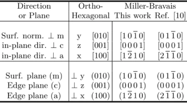
Table S.1 compares the Miller-Bravais indices for vari-ous directions and planes used in this work and in the previous KMC study.
TABLE S.1. Comparison of Miller-Bravais indices used in this work and in the KMC study10.
Direction Ortho- Miller-Bravais or Plane Hexagonal This work Ref. [10]
Surf. norm. ⊥ m y [010] [1 0 1 0] [0 1 1 0] in-plane dir. ⊥ c z [001] [0 0 0 1] [0 0 0 1] in-plane dir. ⊥ a x [100] [1 2 1 0] [2 1 1 0]
Surf. plane (m) ⊥ y (010) (1 0 1 0) (0 1 1 0) Edge plane (c) ⊥ z (001) (0 0 0 1) (0 0 0 1) Edge plane (a) ⊥ x (100) (1 2 1 0) (2 1 1 0)
ACKNOWLEDGMENTS
Work supported by the U.S. Department of Energy (DOE), Office of Science, Office of Basic Energy Sciences, Division of Materials Sciences. Use of beamline 12ID-D of the Advanced Photon Source, a DOE Office of Sci-ence User Facility operated for the Office of SciSci-ence by Argonne National Laboratory, was supported under con-tract DE-AC02-06CH11357.
1E. Perret, M. J. Highland, G. B. Stephenson, S. K. Streiffer, P. Zapol, P. H. Fuoss, A. Munkholm, and C. Thompson, “Real-time x-ray studies of crystal growth modes during metal-organic vapor phase epitaxy of GaN on c- and m-plane single crystals,”
2I. K. Robinson and D. J. Tweet, “Surface x-ray diffraction,”
Re-ports on Progress in Physics 55, 599–651 (1992).
3G. B. Stephenson, J. A. Eastman, O. Auciello, A. Munkholm, C. Thompson, P. H. Fuoss, P. Fini, S. P. DenBaars, and J. S. Speck, “Real-time x-ray scattering studies of surface structure during metalorganic chemical vapor deposition of GaN,” MRS Bulletin 24, 21 (1999).
4A. Munkholm, G. B. Stephenson, J. A. Eastman, O. Auciello, M. V. R. Murty, C. Thompson, P. Fini, J. S. Speck, and S. P. DenBaars, “In situ studies of the effect of silicon on GaN growth modes,” Journal of Crystal Growth 221, 98–105 (2000), proc Tenth Int Conf Metalorganic Vapor Phase Epitaxy.
5P. Kraft, A. Bergamaschi, C. Broennimann, R. Dinapoli, E. F. Eikenberry, B. Henrich, I. Johnson, A. Mozzanica, C. M. Schlep¨utz, P. R. Willmott, and B. Schmitt, “Performance of single-photon-counting PILATUS detector modules,”Journal of Synchrotron Radiation 16, 368–375 (2009).
6Kyma Technologies, 8829 Midway West Rd Raleigh, NC 27612,
USA,http://www.kymatech.com.
7G. Ju, M. J. Highland, A. Yanguas-Gil, C. Thompson, J. A. Eastman, H. Zhou, S. M. Brennan, G. B. Stephenson, and P. H. Fuoss, “An instrument for in situ coherent x-ray studies of metal-organic vapor phase epitaxy of III-nitrides,”Review of Scientific Instruments 88, 035113 (2017).
8G. B. Stringfellow, “Fundamentals of vapor phase epitaxial growth processes,” AIP Conference Proceedings 916, 48–68 (2007).
9M. Lohmeier and E. Vlieg, “Angle calculations for a six-circle surface x-ray diffractometer,” Journal of Applied Crystallogra-phy 26, 706–716 (1993).
10D. Xu, P. Zapol, G. B. Stephenson, and C. Thompson, “Kinetic Monte Carlo simulations of GaN homoepitaxy on c- and m-plane surfaces,”Journal of Chemical Physics 146, 144702 (2017). 11H. M. Otte and A. G. Crocker, “Crystallographic formulae for