Simplified design methods for pipelines subject to transverse and longitudinal soil movements

Publisher’s version / Version de l'éditeur:

Canadian Geotechnical Journal, 32, 2, pp. 309-323, 1995

READ THESE TERMS AND CONDITIONS CAREFULLY BEFORE USING THIS WEBSITE. https://nrc-publications.canada.ca/eng/copyright

Vous avez des questions? Nous pouvons vous aider. Pour communiquer directement avec un auteur, consultez la première page de la revue dans laquelle son article a été publié afin de trouver ses coordonnées. Si vous n’arrivez pas à les repérer, communiquez avec nous à PublicationsArchive-ArchivesPublications@nrc-cnrc.gc.ca.

Questions? Contact the NRC Publications Archive team at

PublicationsArchive-ArchivesPublications@nrc-cnrc.gc.ca. If you wish to email the authors directly, please see the first page of the publication for their contact information.

NRC Publications Archive

Archives des publications du CNRC

This publication could be one of several versions: author’s original, accepted manuscript or the publisher’s version. / La version de cette publication peut être l’une des suivantes : la version prépublication de l’auteur, la version acceptée du manuscrit ou la version de l’éditeur.

Access and use of this website and the material on it are subject to the Terms and Conditions set forth at

Simplified design methods for pipelines subject to transverse and

longitudinal soil movements

Rajani, B. B.; Robertson, P. K.; Morgenstern, N. R.

https://publications-cnrc.canada.ca/fra/droits

L’accès à ce site Web et l’utilisation de son contenu sont assujettis aux conditions présentées dans le site

LISEZ CES CONDITIONS ATTENTIVEMENT AVANT D’UTILISER CE SITE WEB.

NRC Publications Record / Notice d'Archives des publications de CNRC:

https://nrc-publications.canada.ca/eng/view/object/?id=57d06a9c-28ea-47c7-a22d-f88a51091ce5 https://publications-cnrc.canada.ca/fra/voir/objet/?id=57d06a9c-28ea-47c7-a22d-f88a51091ce5

http://www.nrc-cnrc.gc.ca/irc

Sim plifie d de sign m e t hods for pipe line s subje c t t o t ra nsve rse a nd

longit udina l soil m ove m e nt s

N R C C - 3 8 5 8 4

R a j a n i , B . B . ; R o b e r t s o n , P . K . ; M o r g e n s t e r n ,

N . R .

J a n u a r y 1 9 9 5

A version of this document is published in / Une version de ce document se trouve dans:

Canadian Geotechnical Journal, 32, (2), pp. 309-323, 1995

The material in this document is covered by the provisions of the Copyright Act, by Canadian laws, policies, regulations and international agreements. Such provisions serve to identify the information source and, in specific instances, to prohibit reproduction of materials without written permission. For more information visit http://laws.justice.gc.ca/en/showtdm/cs/C-42

Les renseignements dans ce document sont protégés par la Loi sur le droit d'auteur, par les lois, les politiques et les règlements du Canada et des accords internationaux. Ces dispositions permettent d'identifier la source de l'information et, dans certains cas, d'interdire la copie de documents sans permission écrite. Pour obtenir de plus amples renseignements : http://lois.justice.gc.ca/fr/showtdm/cs/C-42

r

I

I '

309

Simplified design methods for

pipelines subject to transverse and

longitudinal soil movements

B.B. Rajani, P.K. Robertson, and N.R. Morgenstern

Abstract: Pipelines are often subjected to transverse and longitudinal movements due to

displacements in the ground causedby landslides. As landslide movements develop. pipelines can undergo transverse and longitudinal displacements and the resistance offeredby the surrounding soil steadily increases depending on the soil characteristics. This resistance reaches an ultimate as the soil reaches failure and develops plastic strains. Two simple analytical solutions have been developed based on this concept: one for transverse movements and another for longitudinal movements. Nondimensional relationships have been developed and are presented in the form of charts. These charts permit hand calculations and rapid verification of structural design of the pipeline and, thus, assess the integrity of existing pipelines located in areas with ground instability. A knowledge of the soil strength and subgrade modulus is required along with pipeline geometry and pipe stiffness to apply the nondimensional relationships. The soil parameters can be measured in situ or estimated using empirical correlations. Worked examples are given to illustrate the proposed methods and to show how various pipe failure criteria can be included.

Key words: pipelines, landslide, transverse and longitudinal movements, design method.

Resume: Les pipelines sont souvent soumis a des mouvements transversaux et longitudinaux dus au deplacements provenants de glissements de terrain. Lorsque les mouvements se developpent, les pipelines peuvent avoir des deplacements transversaux et longitudinaux, avec une augmentation constante de Ia resistance offerte par Ie sol environnant en fonction de ses caracteristiques. Cette resistance atteint une valeur ultime quand Ie sol arrive

a

la rupture et developpe des deformations plastiques. Deux solutions analytiques simples ont ete developpees

a

partir de ce concept, rune pour les mouvements transversaux, l'autre pour les mouvements longitudinaux. Des relations adimensionnelles ant ete developpees et sont presentees SOllS la forme d'abaques. Ces abaques

permettent des calculs

a

la main et une verification rapide de la conception structurelle du pipeline ,et par consequent permettent d'evaluer l'integrite des pipelines existants et silues dans des zones instables. Pour pouvoir appliquer les relations adimensionnelles il faut connaitre la resistance du sol et son module de reaction ainsi que la geometrie du pipeline et sa raideur. Les parametres du sol peuvent etre mesures sur place au estimes par correlations empiriques. On donne des exemples resolus pour illustrer les methodes proposees et pour montrer comment divers criteres de rupture de tube peuvent etre inclus.

Mots

des :

pipelines, glissement de terrain, mouvement transversaux et longitudinaux, methodes de conception.

[Traduit par la redaction]

Introduction

In many parts of the world buried pipelines are required to cross unstable ground where landslides can occur. Therefore pipelines can be subjected to either transverse or longitu-dinal movements due to displacements in the ground caused Received December 2, 1993. Accepted November 17, 1994. B.B. Rajani. Infrastructure Laboratory, National Research Council Canada, Ottawa. ON KIA OR6, Canada.

P.K. Robertson and N.R. Morgenstern, Department of Civil Engineering. University of Alberta, Edmonton, AB T60 207, Canada.

by landslides. As the landslide movements develop, the pipeline can undergo displacement and the resistance offered by the surrounding soil steadily increases depending on the soil characteristics. This transverse or longitudinal loading from soil movements can eventually cause failure of the pipeline.

Once an active unstable slope has been identified, often field monitoring techniques such as slope indicators and strain gauges are used to monitor ground movement and development of pipeline strain, respectively. Installation and monitoring of these sensors in remote areas can be very expensive and impractical, especially if long lengths of pipeline need to be monitored. On the other hand, not all

310 Can. Geotech. J., Vol. 32, 1995

2w

/

free-field slide displacement _{slide displacementatedge}

x

1 1

,-,

1 X 1 ｾ I I I I I , 1

<

I S § X I "61> 1 I ｾ 1 1 I

'.... I'"

1 1 I I 1 1 defonned pipeline

---·b

. x-section

active slopes pose a serious threat to pipeline integrity, since many variables may effect the pipeline-soil interaction, e.g., slide geometry, pipeline and soil properties. Conse-quently, a pipeline designer faces the challenge to first identify the active landslides that pose a threat to pipeline integrity and, subsequently, to determine how much land-slide movement can be tolerated without jeopardizing ser-viceability of the pipeline. This concern would be equally valid for an existing pipeline or a new pipeline routed through a landslide-prone region.

NOVA Corporation of Alberta, Canada, initiated a research program in collaboration with the University of Alberta to study soil-pipeline interaction due to landslide movements. The research was performed in several phases. The first phase reviewed the available literature on spring-slider models for soil-pipeline interaction analyses and field testing techniques for determination of the required soil parameters. The second phase involved a parametric study to determine the sensitivity of pipeline integrity to variations in soil parameters for transverse landslide loading. The results of the second phase showed that the transverse pipeline deflection profile, due to the landslide loading, essentially follows a double curvature pattern on either side of the landslide interface. The study showed that the pipeline response was controlled predominantly by the soil strength and that soil stiffness had little influence. The study also showed that for the pipes analyzed (NPS-24 andNPS-48; NPS stands for "nominal pipe size" and the size is specified in inches) the pipelines could deflect large amounts before reaching failure, where failure was defined as 0.5% compression strain. Complex finite element cal-culations were performed in the second phase to study the sensitivity of pipeline integrity to variations in soil eters. A preliminary attempt was made to identify a param-eter that could characterize the soil-pipeline behaviour during landslide movement. However, further development

longitudinal section

of this parameter was found to be difficult because of the complexities of the numerical studies required to encompass all the expected variables. Consequently, an analytical solution was investigated and developed as part of the third phase of the study to better understand the influence of all the main variables. As part of the fourth phase of the study, a similar analytical solution was developed for longitudinal loading.

This paper presents the results of this study on the trans-verse and longitudinal loading of pipelines. Analytical solutions previously developed for the uplift behaviour of a shallow pipeline embedded in an elasto-plastic medium are adapted to obtain the transverse response. The simple analytical solution for longitudinal soil loading is also described. The use of these solutions is illustrated using worked examples.

Analytical soil-pipeline interaction:

transverse movement

During the second phase of this research project (Gale et at. 1989) complex numerical studies using the finite element code ADINA were performed to understand the basic pipeline-soil interaction for landslide movements. As previously mentioned, since the results of the second phase showed that the transverse pipeline deflection profile due to the landslide loading essentially follows a double cur-vature pattern, it suffices to analyze only half of the pipeline and prescribe the end of the pipeline at the edge of .the landslide to half of the free-field landslide movement. Free-field landslide movement is defined here as the land-slide movement that would take place in the absence of any restraints. A preliminary attempt was made to identify a parameter that could characterize the soil-pipeline behaviour during landslide displacement. For pipelines with the same material stress-strain behaviour, internal

Rajani et al.

pressure, and failure criteria, a soil-pipeline strength param-eter (ess) was defined based on the shear strength of the soil

r

and the diameter and wall thickness of the pipeline. Hence. . soils and pipelines with the same value of ess could be expected to reach failure at the same magnitude of landslide movement.

Further development of this parameter was found to be difficult because of the complexities of the numerical stud-ies needed to encompass all the involved variables. It was felt that to better understand the influence of the main variables, the development of an analytical solution was required. Consequently, an analytical solution was developed that traces the sequence of events that takes place as a result of the interaction between the pipeline and the sur-rounding soil as the landslide movement monotonically increases. These events can be summarized as follows: on initial landslide movement, the buried pipeline as well as the soil behave elastically; as the landslide movement increases, ultimate passive resistance will be developed in part of the surrounding soil medium but the pipe will remain elastic; on further landslide movement, a plastic ｨｩｮｧｾ or wrinkles begin to develop in the pipeline depending its structural characteristics. The solution was based on an elastic pipeline embedded in an elastic-perfectly plastic soil, and full details are given by Rajani and Morgenstern (1993). The solution incorporates all the major variables that playa significant role in the soil-pipeline interaction. A schematic representation of the transverse movement of a pipeline due to a landslide is shown in Fig. l.

The attractiveness of an analytical solution based on a pipe embedded in an elastic-perfectly plastic soil is the flexibility of the solutions for a broad range of applications. The resulting solutions depend on the total soil resistance per unit length of pipe (R) developed due to movement. Therefore, other solutions can be developed for different boundary conditions provided a suitable total soil resistance can be input to represent the given boundary condition (Rajani and Morgenstern 1993).

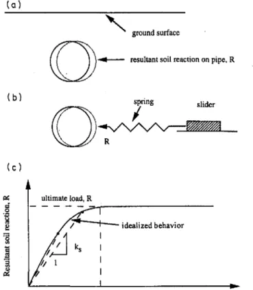
Figure 2 illustrates the concept of an elastic pipeline embedded in an elasto-plastic soil to represent the real field condition. The soil is assumed to be an elastic-perfectly plastic isotropic, homogeneous medium; whereas, the pipe is assumed to be a linear elastic beam. The key parameters that control the analytical solution are the soil stiffness, resistance per unit length of pipe represented by the soil subgrade modulus, k" the ultimate soil resistance, R, and the pipe stiffness represented by the flexural modulus, EI, of the pipe. The ultimate soil resistance is dependent on the soil strength and the prevailing boundary conditions. Typically, the ultimate force per unit length, R, resistance available for clay corresponding to the undrained state can be expressed by [1] R =_Nebsu cohesive soil

where Su is the undrained strength and

N

_eis a horizontal

bearing capacity factor for cohesive soils. The pipeline is embedded at a depth, h, below the ground surface and has a diameter, b, and wall thickness, t. The embedment depth, h, is measured from the ground surface to the base of the pipeline, as shown in Fig. I.

Numerical solutions developed by Rowe and Davis (1982) for cohesive soils can be used to evaluate the ultimate

311 Fig. 2. Spring-slider representation of soil-pipeline

interaction. (a) Pipe displaced to the right. (b) Spring-slider representation. (c) Force-displacement relation.

(a) ' " ground surface

0-

ｾＢＧＢＢＬｯｯｬｬ

"'0000000"". R

ｯｾ

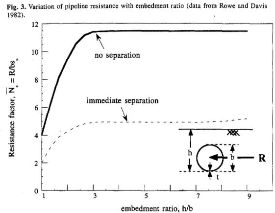
(c) ultimate load, R ｾＭＭＭＭＭＭＭＭＭＭ idealized behavior lransverse displacement,W

soil resistance developed due to the transverse movement of the pipeline. Rowe and Davis (1982) showed that the ultimate soil resistance is dependent on the embedment depth and the degree of bonding between the back of the pipeline and the soil. Figure 3 shows the solutions devel-oped by Rowe and Davis (1982). For an embedment ratio (h/b) of 2, the ultimate soil resistance, R, is essentially 4bs_u when the soil separates from the back of the pipe, and 9bs_u when no separation occurs.

The transverse (uplift or lateral) response of the pipeline to landslide movement was obtained by solving the general analytical solution described by Rajani and Morgenstern (1993) Ｈｾｲ particular values of pipeline-soil resistance factors, No, developed by Rowe and Davis (1982) (Fig. 3). In this solution, the free-field landslide displacement is designated as 2w, and considering that the pipeline dis-placemellt profile has a double curvature, the transverse displacement of the pipeline at the edge of the landslide is w, which is half of the free-field landslide displacement as shown on Fig. 1. Concurrently, it is also assumed that the sliding mass has sufficient transverse extent that it is ade-quate to analyze the pipeline-soil interaction near one edge of the landslide. It is noted that the general analytical solu-tion described by Rajani and Morgenstern (1993) was first applied to evaluate the behaviour of the uplift response of pipelines. The load, P,applied to the pipeline is a theoretical load that causes the pipeline to deflect(w) at the edge of the landslide. The solution is generalized for pipeline defor-mation when embedded in an elasto-plastic soil. The resolution

r

I

312 Can. Geotech. J., Vol. 32, 1995

Fig. 3. Variation of pipeline resistance with embedment ratio (data from Rowe and Davis 1982). 12 . . - - - , II 8

no separation

immediate separation

-

-

-

- -

ｾ

- -

-

- - -

-

- - - -

-

-

- -

-6 4

,.

,. / I 2 10

ｾＮ

ｉｚｾ

o

1 _{7 9}

embedment ratio, h/b

Fig. 4. Range of nondimensional load - displacement curves for typical pipeline embedments subject to transverse movement due to landslide.

20

..---=---=:::::::0---,

N =4 o _ - - - N = 3 N_e

=

11.42 ｾ _ _ _ _ _{_ ")._} N c=lO _ _ h

ir

No = 8 .

J-

-l-

_1

ｎ］Ｖｾ

N_c

=

5.14

v

=

0.35 (jl =0

y=O

5 10 15

End displacement,

W

=

k

_,

w/s

"

[2]

of the analytical solutions for different values of

N

e and

transverse load can be summarized by two sets of char-acteristic curves, as explained in the appendix and shown in Figs. 4 and 5. Figure 4 shows the characteristic curves for transverse loading in terms of nondimensional end load,

P,

and the associated nondimensioEal end displace-ment,

w.

The nondimensional end load.P, is defined as

p

= Pf3

where P is applied load at the edge of landslide,

f3

(= ｾｫＬ｢ｉＴｅｬＩ is a parameter whose reciprocal is charac-teristic length of soil-pipeline, k, is soil subgrade modulus, Eis pipeline Young's modulus, and 1is pipeline moment of inertia. The parameter

f3

is a ratio of soil subgrade modulus and beam stiffnesses. The reciprocal of f3 is the teristic length of the soil-beam system. Thus, the charac-teristic length is a measure of the interaction between the beam and the elastic foundation.

I

i .

I

Rajani et al. 313

Fig. S. Range of nondimensional maximum moment - displacement curves for typical pipeline embedments subject to transverse movement due to landslide.

ｾ 2,--- ---. 1.5 1 0.5

v

=

0.35 c1>

=0

1=0

N =2 o N=lO N

=

11.42 c

End displacement,

W

= k

w/s

• u

The nondimensional end (edge) displacement, W, is defined as

3] - ｾｷ

( w =

-Su

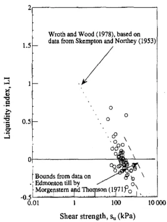
Fig. 6. Relation between shear strength and liquidity index of Alberta tills.

2 . - - - . . . ,

[4]

-0.5L-..."'"--...L.-...ｾ ...ｾ ...

O.ol 100 10 000

Shear strength,Su(kPa)

relative to the pipe. A high soil resistance will produce large stresses in the pipe for any given ground displacement. The characteristic curves (Fig. 5) represent the complete generalized solution for an elastic pipeline embedded in an elasto-plastic soil for all combinations of soil and pipe stiffness, embedment ratios, pipe geometry, and soil strength.

o o . 0

Wroth and Wood(1978),based on data from Skempton and Northey (1953)

/

1.5

....

...J

.g

.S

C

:a

_0.5 'S 0-;J 0 Figure5 shows the characteristic curves for transverse

loading in terms of a nondimensional maximum moment in the pipe,

M,

associated with various nondimensional end displacements,W. The nondimensional moment

M

is defined as

Mfj

P

whereMis the maximum moment developed in the pipeline due to the applied end loadP.

Typically large diameter pipelines in Alberta, Canada, are placed so that the soil cover is at least equal to the diameter of the pipeline. This means that the pipeline embedment ratio, hlh, defined as the ratio of depth to the base of the pipeline and the soil cover, is typically about 2 or very near this value. Based on solutions prOVided by Rowe and Davis (1982) (Fig. 3), the resistance factor

N

_ecan vary from 4 to 9 depending on whether soil separation occurs or not at large displacement. Most pipelines in Alberta are placed in relatively stiff glacial till deposits. When these pipelines are subjected to transverse move-ments due to ground mOVemove-ments it is expected that sepa-ration will occur between the soil and the back of the pipe at large displacements. Initially, for small displacements the soil can be expected to move with the pipe (Le., no separation). However, separation is likely with large move-ments. Consequently, the

N

_evalue would be high (around 9) at small displacements, whereas, separation may occur with large displacements when the

N

_evalue would be rel-atively low (around 4).

In general, the most severe ground loading conditions for a pipeline will be when the soil is strong and (or) stiff

Failure of the pipeline can be defined in terms of a maxi-mum moment (M) or maximum stress, cr, where

Mb [5] cr =

-21

and 1 is the pipeline moment of inertia.

The use of these characteristic curves requires the

knowl-edge of the soil strength (s,) and subgrade modulus (k,) along with pipeline geometry and stiffness. In general, the pipeline characteristics are well defined in terms of b, I,

h, E, and 1. The soil parameters can be measured in situ or

estimated using empirical correlations, such as shown in

Fig. 6 (Rajani et aJ. 1992).

While the discussion of the analytical solution and cor-responding characteristic curves has been in particular

reference to cohesive soils, the characteristic curves are

general enough to be applicable to pipelines buried in

granular soils. The ultimate soil resistance for a frictional

soil (sand) is given by (Committee on Gas and Liquid Fuel Lifelines 1984)

[6] R = Nqhb'9,(h -

%)

frictional soil

whereNqh is horizqntal bearing capacity factor for frictional soil and

'9,

is effective unit weight of soil. The comparison of eq. I for cohesive soils with eq. 6 for granular soils indicates that the characteristics curves (Figs. 4 and 5) can still be used for analysis of pipelines buried in granular soils if

N,

and s, are substituted by N_qh, and

'9,

(h - b12), respectively.

For most soil conditions, the undrained rapid response

will generally produce the highest resistance and will, therefore, be the most conservative. In general. the backfill material will have a lower strength than the surrounding natural ground. For preliminary design it would be more prudent to apply the shear strength of the natural ground, since this would produce larger calculated stresses in the

pipe for a given ground movement. However. in critical regions where large transverse soil movements are

antici-pated the backfill material should be as weak as possible and the pipeline trench as wide as possible. This would

allow maximum movement of the natural ground without

producing high stresses and strains in the pipe.

Although not immediately apparent from Figs. 4 and 5, the soil strength has the most dominant affect on the pipeline response. The soil stiffness in terms of a subgrade modulus, k" has a large effect at small displacements(w) but a much smaller effect at large displacements when the soil reaches failure and becomes plastic. The soil subgrade modulus can be determined from either full-scale tests, plate loading tests, or estimated using empirical correlations. If no laboratory data are available, than the range of possible values can be estimated from Table I, as suggested by Bowles(1977) and Poulos and Davis (1980). The soil sub-grade modulus indicated in Table I does not account for pipeline size effects since its influence is probably over-shadowed by the range of soil properties encountered along the linear extension of the buried pipeline. It will generally be sufficient to estimate k, using Table 1 since the soil subgrade modulus values have only a small influence on the resulting design. The undrained shear strength can be

deter-mined from either laboratory or in situ tests or estimates can

be obtained from index properties, as suggested in Fig. 6.

The current analytical solutions shown in nondimensional

form in Figs. 4 and 5 are based on assumptions that the displacements and strains experienced in the pipeline are small. As long as the transverse displacements are small in comparison with the diameter of the pipeline, the dominant behaviour of the pipeline at the interface of the sliding

mass is flexure. As soon as the transverse displacement is significant in comparison to the diameter of the pipeline.

the mode of behaviour of the pipeline changes from flexure to extension. An indicator for performing a large defor-mation analyses is when the slope along a deformed pipeline exceeds 117, i.e., dwldx > 117. This requirement derives

from the approximation used in the definition for curvature

for the analysis of beams. The evaluation of the response for large displacements requires that the "cable-like"

behav-iour of the pipeline must be taken into account since

con-siderable tension will be induced in the pipeline. The

result-ing extension and bendresult-ing may be significant to cause

plastic strains in the pipeline. While a large displacement solution is complex (Rajani et al. 1992), it is likely that

Rajani et al.

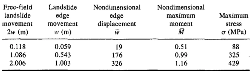
Table3. Key displacement-stress history points for a 1.22 m pipeline subjected to

transverse landslide movement.

ｾＭＭＭＭＭＭＭＭＭＭＭＭＭＭＭＭＭＭＭＭＭＭＭ

Free-field Landslide Nondimensional Nondimensional

landslide edge edge maximum Maximum

movement movement displacement moment stress

2w (m) w (m) iii

Ai

et(MPa)

0.118 0.059 19 0.51 88

1.086 0.543 176 0.99 325

2.006 1.003 326 1.16 429

315

the small strain, small displacement formulation discussed here will be adequate for most design problems as long as landslide movements do not significantly exceed the pipeline diameter.

Worked example: transversal movement

A worked example is presented to illustrate the application of the characteristic curves shown in Figs. 4 and 5. The pertinent pipeline and soil characteristics are shown in Table 2.

The data for this worked example is similar to the one that served as the baseline case data set used for the para-metric study of soil-pipeline interaction for pipelines cross-ing landslides carried out by Gale et al. (1989). There is no significance to the fact that undrained shear strength for the clay in this worked example does not represent a stiff clay typically encountered in Alberta.

Only half of the free-field landslide movement is assumed to occur at the edge of the landslide since the transverse pipeline deflection profile has a double curvature. A series of different edge displacement values can be assumed to calculate the corresponding maximum moment(M) and stress (et) in the pipeline. For a free-field landslide move-ment (2w) of. for example, 1.08 m, the landslide edge movement, w,is 0.54 m and, consequently, the non-dimensional displacement isiii=k,w!s, = 176. Using Fig. 4 and taking the cha.!:acteristic curveN, = 5, the nondimen-sional end load isP= Pfi!bs,= 8. Hence, for this pipeline at this particular displacement, the end load,P, is l,;l MN. Using Fig. 5 and taking the characteristic ｣ｾｲｶ･ N, = 5, the nondimensional maximum moment is M = Mfi!P =

0.99. SinceP was already determined from Fig. 4 in the

previous step, it is now possible to calculate the

maxi-mum moment, M, which is 8.59 MN·m, and corresponding stress (et = Mb!2l) in the pipeline is calculated to be 325 MPa.

Subsequently, other key displacement-stress history points can now be identified, as indicated io Table 3. Yield-ing in steel commences typically in the range of 0.1 to 0.2% strain, which corresponds to a stress range of 200-400 MPa. In practice. loading imposed on the pipeline

as a result of landslide movement is considered as a

sec-ondary loading condition and, typically, the compressive (wrinkling) strain is limited to about 0.5% (Canadian Stan-dards Association 1992) for steel pipelines in the pipeline industry. This means that for landslide displacements greater than I m, the analysis needs to be modified to account for

the nonlinearity in the pipeline as opposed to that in the soil only.

As explained earlier, the level of strain developed at any particular position in the pipeline will depend on the magnitude of landslide movement as well as on the distance of the point from the edge of the landslide, Consequently, the analysis of this particular problem indicates that portions of the pipeline exceed the yield strain as soon as the land-slide movement is greater than 1 m. Recent (Rajani 1992) model experiments have shown pipelines can undergo severe compressive strains, i.e., greater than 0.8% strains without rupture. The typical strain at first yield in tension for steel is about 0.10-0.15%.

Since the present analytical solution does not account for nonlinear (plastic) deformation of the pipeline, an approx-imate procedure is proposed. In practice, yielding of pipeline initiates at one particular section and, thereafter, yielding extends to adjacent sections on further deformation. Analy-ses of pipelines using practical pipeline and soil data indi-cate that the maximum stress generally develops within the first 5 diameters of the pipe from the edge of the land-slide. An upper bound estimate of the strain can be obtained if it were to be assumed that the whole length of pipeline in the vicinity of the landslide edge yields at the same instant. Under these circumstances, the pipeline can be reanalyzed using a reduced pipe stiffness recognizing that the procedure proposed here is certainly not rigourous but provides a reasonable estimate. In this procedure, it is fur-ther assumed that the solution for a pipeline embedded in an elasto-plastic soil continues to hold even though the pipeline behaviour in tension and compression beyond yield or wrinkling is not the Same. In the approximate pro-cedure, an equivalent elastic modulus for the steel pipeline is used on the basis that failure is defined in terms of lim-iting critical comptessive strain to 0.5% rather than the yield stress (Committee on Gas and Liquid Fuel Lifelines 1984; Canadian Standards Association 1992).

Since steel has an elastic modulus (E,) of 207 GPa, yield stress (ety) for steel is 310 MPa if it is assumed that steel yields at a strain of 0.15%. Thus, the equivalent secant modulus(E,,,,) of steel reduces to 62 GPa at a strain of 0.5%. Subsequently, the pipeline can be reanalyzed except that the equivalent secant modulus (E",) is used instead of the elastic modulus (E,). Parameter

fi.

the rec-iprocal of characteristic length, is 0.21 m-'. Therefore, a free-field landslide displacement(2w) of 2 m will produce a nondimensional edge displacement (w) of 325. Using Fig. 4

(N,

= 5), the nondimensional end load

(P)

is 9.2,

316

Fig. 7. Pipeline subjected to a longitudinal planar slide:

(a)plan view, (b) section view. lQ)

(b)

sliding mass

stable ground

which corresponds to an end load (P) of 1069 kN. Using Fig. 5 (N,

=

5). the nondimensional moment (M) is 1.16, and, therefore, M

=

5905 kN·m and IT

=

224 MPa. For a ｦｲ･･ｾｦｩ･ｬ､ landslide movement of 2 m, the maximum strain developed is 0.36% when a reduced secant modulus is used in the analysis. Therefore, this approximate analysis indicates that if the development of plastic or wrinkling strains is tolerated, landslide movements larger than 2 mean be accommodated before the tensile or compressive strain exceeds 0.5%.

Alternate applications of the

analytical solution

Though the characteristic curves shown in Figs. 4 and 5 were developed for transverse movements of a pipeline embedded in a soil at shallow depth, they can be applied to analyse alternative beam-soil interaction type problems.

The solution can be modified to account for the uplift behaviour of pipelines or the lateral loading of vertical piles if the ultimate soil resistance values are modified to account for the different boundary conditions. An example of the solution for the uplift behaviour of pipelines is given by Rajani and Morgenstern (1993). For the uplift behaviour of pipelines, the equivalent resistance factor,F(, ranges

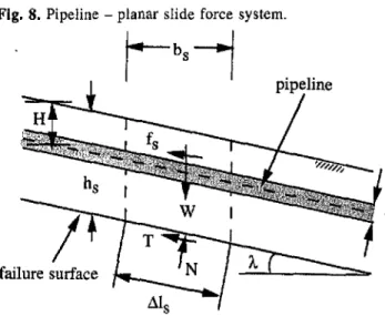
Can, Geotech. J., Vol. 32, 1995 Fig. 8. Pipeline - planar slide force system.

b

failure surface

from about 2 to 12 depending on the separation of soil beneath the pipe. For laterally loaded piles, the boundary conditions are different, with the free surface perpendicular to the pile. For laterally loaded piles, the resistance ｦ｡｣ｾ tor

No

ranges from 9 to II. Hence, the curves shown in Figs. 4 and 5 can be applied to other applications that can be represented by an elastic pipe embedded in an elasto-plastic material subjected to lateral loading.

Soil-pipeline interaction: longitudinal

movement

When pipelines cross river valleys they are often constructed such that the pipeline follows the slope of the valley wall. If slope instability occurs in the valley wall, the pipeline will be subjected to longitudinal soil-pipeline interaction. This longitudinal interaction will induce longitudinal strains in the pipe that could lead it to failure.

The failure of the pipeline at the Simonette River Cross-ing in 1978 prompted an· inquiry of the observed failure. Studies undertaken by M. Rizkalla and M. Moschopedis (private communication. 1989) concluded that failure was probably caused by a combination of operating, bending, and residual stresses. One of the mechanisms that was studied was the longitudinal stresses imposed on the pipeline as a result of longitudinal slide movement. The longitu-dinal stresses or strains were estimated by the use of a finite element model. However, during the design stage the estimate of probable stresses imposed on a pipeline, as a consequence of a landslide hazard, is generally not justified by making use of a relatively detailed model because of uncertainty in the soil properties and landslide geometry. In the following sections, the development of characteristic curves for longitudinal movements is described. A worked example is given to illustrate the application of the method to evaluate the longitudinal response of a pipeline.

A significant amount of axial force can be exerted on a pipeline as a consequence of the longitudinal movement of a sliding soil mass. As an initial approximation, it is reasonable to assume that the sliding mass is planar and has finite dimensions of width (W,) and length (L,), as indicated in Fig. 7. The anticipated mechanism envisaged

Rajani at al. 317

strain,E axial displacement, u

( a )

Approach 2: Axial soil-pipeline interaction analysis

in stable mass A

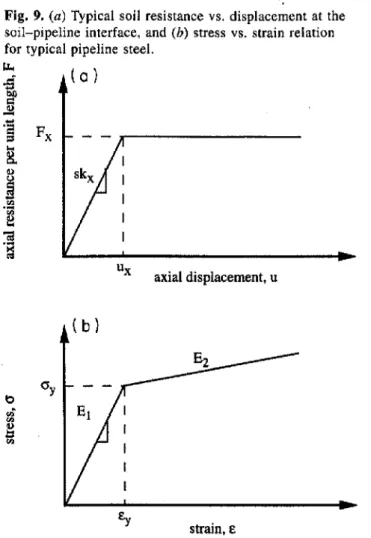
The second approach would be to estimate the net force at the interface (Po) by looking at the force displacement interaction of the pipeline embedded in either the non-moving soil mass A or the moving mass B. If a force Po is imposed at the slide interface that increases monotonically, then it will be supported by the development of soil-pipeline resistance. The resistance along the interface will depend on the developed displacements and, hence, the stress in the pipeline can be traced as a function of the net force, Po. The soil is represented as an elastic-perfectly plastic material (Fig. 9a) and the pipeline itself is considered to follow where Su is the undrained shear strength on the failure

plane in the slope. Thus, the soil-pipeline resistance can be determined if the slide characteristics and soil properties can be reasonably estimated. If the slide length is L_s' the total force, Po,at the interace of moving-nonmoving masSes is [14] Po::::_IsLs

This approach assumes that the slope is just at failure (Le., factor of safety of 1.0) and that the full shear strength has not been developed between the soil backfill and pipe, Le., there is no slip between the soil and the pipe. The limiting condition exists when the strength between the soil backfill and pipe is fully developed and slip occurs along the soil-pipe interface.

Fig. 9.(a) Typical soil resistance vs. displacement at the soil-pipeline interface, and(b) stress vs. strain relation for typical pipeline steel.

f.t.

,

'S

₌₌

_F

_x

8.

Approach 1: Limit equilibrium analysis of sliding mass B

One approach would be to use limit equilibrium to estimate the net force exerted at the interface of the moving-non-moving soil masses. It is often reasonable to assume that the slide is planar and that an estimate of the slide depth, h_s' can be made from conventional slope stability analysis. The side forces on the slide shall be neglected in the following analysis. The forces acting on a typical slice in the slide with the embedded pipeline within the sliding mass are shown in Fig. 8.The resolution of forces parallel and nor-mal to the slope, A, result in the following equations: [7] !::.Isfs

+

T= W sin A

[8] N;;;;: W cos A

where

t.

is the resulting soil-pipeline resistance per unit length of pipeline, W is the weight of the sliding mass per unit length of pipeline, Nand Tare the soil forces acting on the failure plane in the slope, and !::.I, is the unit length of pipeline.

The failure criterion for the surrounding soil is assumed to be of the Mohr-Coulomb type and can be expressed as [9] T ;;;;: C

+

0" tan <1>'

where cand

c!>'

are the effective stress cohesion and friction angle parameters, respectively, of the soil along the failure plane in the slope. The following two equations relate the mass of the slide slice with geometry:

[10] W = _pghsb,Ws

[11 ] bs :::: t1l_scos A

If slide movement occurs then the driving force must equal to or exceed the resisting forces, i.e., factor of safety is one as in conventional stability analysis. The resulting soil-pipeline resistance per unit length of pipeline,

Is'

is given by

[12]

Is

=I'_sh_sW_s(sin A cos h. - cos2h. tan <1>') - cW_s where "Is is the soil unit weight, hsis depth of the landslide,

W_s is the slide width, h. is slope of soil sliding mass. If the soil strength for the soil along the slope failure plane is represented by the undrained shear strength

(c!>'

=0, C=su)'

the expression becomes

[13] Is::::l',h,W, sin h. cos h. - suW,

is that the movement of the sliding mass B and the firm embedment of the pipeline in a stable nonmoving mass A ｾｲ･ｳｵｬｴｳ in a net force at the interface to overcome the slid-ing resistance between the pipeline and the surroundslid-ing soil. A key design question follows: how large a slide movement can be tolerated before pipeline failure occurs if the pipeline and soil characteristics can be estimated rea-sonably well. The problem can be solved using two different but related approaches. One approach would be to use limit equilibrium to estimate the net force exerted at the interface of the moving-nonmoving soil masses. The second approach would be to .estimate the net force at the interface (Po) by looking at the force displacement interaction of the pipeline embedded in either the nonmoving soil mass A or the moving mass B.

318

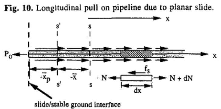
Fig. 10. Longitudinal pull on pipeline due to planar slide.

ｾ x

.. x

the nonlinear strain hardening characteristics of a typical steel pipeline (Fig. 9b). Typical ultimate axial resistance per unit length (Committee on Gas and Liquid Fuel Life-lines 1984), Fx' for a pipeline and the surrounding soils

(clay and sand) can be expressed as [15J Fx

=

rrbc:x.s_u for clay

[16] F_x

=

O.5rrb;Y,H(1

+

Ko)tan 8 for sand

where Su is the undrained shear strength of the soil around

the pipe, b is pipeline diameter, ex is the adhesion factor, K_o is the coefficient of earth pressure at rest, 8 is the interface friction angle between the pipeline and soil,

;y,

is the effec-tive unit weight of soil, and H is the depth from ground surface to the centre of the pipeline. The limiting elastic soil displacement, u_x' is typically 5-10 mm (Committee on Gas and Liquid Fuel Lifelines 1984). The axial sub grade modulus, k_x' is then given by

[17] F

=

kxwrrb for u:$; U_x

whereF is axial force per unit length, 'lTb is the perimeter of the pipeline and uis the axial displacement. Equation 17 expresses the relationship between the soil resistance and axial displacement when the soil response is still elastic. It is worth pointing out that in the first approach using limit equilibrium analysis, the failure takes place along a soil-soil interface since it is assumed that mass B (Fig. 7) is undergoing downward movement and, thus, it permits the evaluation of the overall mobilized soil-pipeline resis-tance per unit length to calculate the axial force exerted on the pipeline at the slide - stable ground interface. In approach 2, the soil-pipeline resistance is evaluated on the basis of on-going soil-pipeline interaction and accounts for the fact that the soil in the stable mass may be different from that in the sliding mass.

The overall pipeline response can be proportioned to three distinct stages of soil-pipeline interaction as the lon-gitudinal movement is monotonically increased. These three stages are (I) both soil and pipeline response are elastic; (2) pipeline response is elastic but sufficient dis-placement has taken place as to develop ultimate soil resis-tance (soil is in the plastic state), and (3) both soil and pipeline are in an elasto-plastic state. The response will be characterized by load and displacement at the interface of the moving and nonmoving masses. The surrounding soil can be represented by axial springs.

Analytical solutions were developed for each stage iden-tified above. Appropriate differential equations were estab-lished and solved for the corresponding boundary condi-tions. Full details are given in Rajani et al. (1992). These

Can. Geotech. J., VoL 32, 1995 analytical solutions were developed in terms of non-dimensional longitudinal jisplacement and load parame-ters, Uo ;::: rrbkxuJFxandP

=

'YPJFx' respectively, where

rrb is the perimeter of the pipeline, k_xis the axial sub-grade modulus, U_{o and Po are the axial displacement and}

load at the landslide interface, and Fxis the axial soil resistance defined in either eq. 15 or 16. In addition, the solutions are a function of the reciprocal of the axial char-acteristic length, 'Y,

_

ｾＧｬｔ｢ｫｸ

'Y -

-EtA

where E₁is the elastic modulus for pipeline andA is the cross-sectional area.

(1) Soil and pipeline are both elastic

Figure 10 shows a free body diagram for axial response of a pipeline subjected to an end load, Po' As long as the longitudinal movement is less than the ultimate longitudinal movement required to induce unrecoverable strains in the soil, Le., U :$; u_x; the following nondimensional equation results:

[18] U_o

=p

whereU_ois the nondimensional longitudinal edge displacement.

(2) Pipeline response is elastic and soil resistance is plastic

If the load level is high enough then the ultimate soil resis-tance will be developed along the pipeline-soil interface for a portion of the pipeline defined by

x.

Hence, over the portion of the pipeline defined by X, the soil response is elasto-plastic. The axis s-s, therefore, distinguishes between the elastic and plastic soil response portions (assume

x

_p

=

o

in Fig. 10). For the plastic soil response portion, the analysis is similar as before except that the axial resistance is independent of longitudinal displacements. The corre-sponding response can be described by the following non-dimensional equation:

[19] 2u_{o ;:::} 1

+

[>2

For loads less than Po :$;FJ'Y the elastic displacement can be expressed in the same form as in [18}.

(3) Pipeline response is elasto-plastic and soil resistance is plastic

The procedure for this phase of the analysis is similar to before except that we have an additional zone where the pipeline itself is undergoing strain hardening. The load-displacement response can then be followed at the interface of the moving-nonmoving masses and can be expressed in nondimensional form as indicated below:

,

Ie "I') -2 - I [20] uo ;:::

-T(1 -

"1')

+

2

P

+

KP(l - "1')

+

2"

where"I')

=

E_lfE₂ is the ratio of elastic to hardening moduli of pipe, K

=

('lTbEvkxI'YFx) is the soil-pipeline stiffness parameter, Cy is the pipeline strain at yield(=0'/E1(Fig. 9b»).

Equation 20 provides an opportunity to examine the relation between the longitudinal load and corresponding displacement for a range of parameters. The sensitivity of

r

i

I

i

Rajani et al.

Fig. 11. Nondimensional characteristic curve for axial load-displacement for longitudinal soil-pipeline ｩｮｾｲ｡｣ｴｩｯｮＮ

500ＬＭＭＭＭＭＭＭＭＭＭＭＭＭＭＭＭＭＭＭｾ｟Ｎ

319

, ,

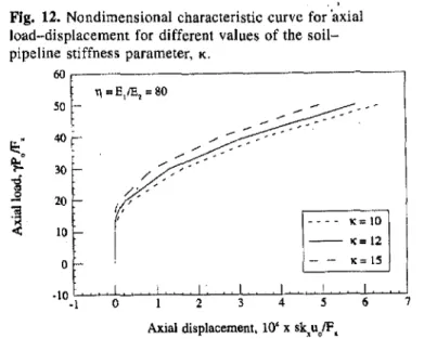
Fig, 12. Nondimensional characteristic curve for 'axial load-displacement for different values of the soil-pipeline stiffness parameter,K.

60,....---,

7 ---- K=IO --1C=12 1C= 15 / " /.ｾ , I, ' I

so

ｾＺ 40 ｾ 30

]

₂₀

ｾ

10 0 ·10 -I T\

=

E,IE,

=

80

-

-plastic soil/-plastic pipe

I

11

=

E/El=80 100f- , / / I 200 ,.;-300 \-,

, elastic soil/elastic pipe

ＴＰＰｾＯ

.

plastic soil/elastic pipe

i-

--Axial displacement, 104

.x sk,uolF, Axial displacement. 104x sk,uolF.

[22] the relationship to the nondimensional parameters'll and

K can also pe easily examined. If typical values for elastic

and hardening modulus for steel are used, then11 will be about 80 and K varies according to the undrained shear strength, adhesion factor, and other parameters that intervene in the definition ofK. However, for typical soil and steel

properties, K should vary in the range of 5-20 with lower

values for stiffer soils. For the present study, K was esti-mated to vary in the range of 10-15.

The resulting nondimensional axial load - displacement characteristic curves are shown in Fig. II. Figure II shows three sets of curves that represent the three main conditions:

(1) both soil and pipeline response are elastic; (2) pipeline response is elastic but sufficient displacement has taken place as to develop ultimate soil resistance (soil is in the elasto-plastic state); and (3) both soil and pipeline are in an elasto-plastic state. It is evident that the largest forces are produced by the somewhat trivial case when the soil and pipe are considered to be elastic. This is certainly too con-servative for most pipeline designs. The next worst loading is when the pipe is assumed to be elastic but the soil has become plastic in the areas of large movement, i.e., close to the interface between the stable and sliding soil masses. The application of this condition (Fig. II) would also result in a conservative pipeline design. A more realistic design would result from the application of the curve that represents the condition of a plastic soil and elasto-plastic pipe. This condition requires some knowledge of the K parameter.

However, Fig. 12 shows that when the soil and pipe are in the elasto-plastic state the K parameter plays a minor role in

the load-displacement response. Hence. it is reasonable to assume a value ofK == 12 for most designs.

Values of the axial subgrade modulus k, can be estimated by assuming an axial displacement of 5 mm to reach the maximum axial resistance per unit length. F_x' Hence.

k == Fx _{_1_ (kN·m-}2_{.m-I )}

, 'ITb 0.005

The adhesion factor, a, can be estimated from data obtained for axial pipeline behaviour and this data has been recently summarized by Siaden (1992).

Comparison of proposed longitudinal

method with other solutions

Rizkalla and Mclntye (1991) presented a simplified expres-sion relating the stress in a pipe due to longitudinal move-ments of a clay slope. This section compares the non-dimensional analytical solution presented in eq. 19 with that obtained by Rizkalla and McIntye (1991).

For a clayey soil the nondimensional expressions defined earlier become (where F_x

=

'Ttbas_u)

[21] U_o ==

kxu

o

as_u

p::::

Po'Y

'ITbas_u

For the case of an elastic pipe and plastic soil the rela-tionship given in eq. 19 holds. Substituting [21] and [22] into [19], the resulting equation for a clayey soil is

[23] Uo ₌₌

ｾＨｆＬＱａ

J

+

ｾｵｸ

where U_xis axial displacement when soil and pipe are both

elastic (Fig. 9).

Rizkalla and Mclntye (1991) have proposed a similar relationship for a clayey soil as follows:

[241 0" "'.

(U

o

;Ef2

Replacing the stress (0")for the axial load (P) the above expression becomes

p2

[25] U == _ 0 _

o FxE1A

The expression given by Rizkalla and Mclntye (1991) assumes an elastic pipeline and plastic soil. It also assumes that the displacement U_o at the edge of the landslide is

twice the landslide movement, since the soil is assumed to move equal amounts about either side of the slide inter-face. Hence, the expressions derived in this study (egs. 19

ｾ

I

320

Can. Geotech. J., Vol. 32, 1995

Table 4. Summary of soil properties. landslide mass geome-try. and pipeline data for longitudinal analysis of pipelines.

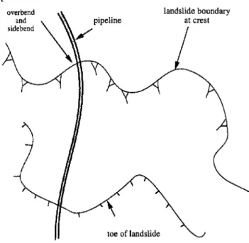
Fig. 13. Plan view of a typical pipeline traversing a potential landslide area.

Worked example: longitudinal movement

The objective of this worked exampled is to illustrate the application of the proposed nondimensional characteristic curves for longitudinal movement of a unstable slope. It is important to note that, in general, pipelines will not be predominantly in a straight line going down slope (Fig. 13) but an overbend and a sidebend can also exist. Therefore. it will not always be possible to attribute the failure totally to longitudinal movement alone.

In the analytical procedure discussed above. the geometry of the mass movement (Fig. 14) can be idealized to a rec-tangular block and average dimensions can be established by judgment from some data on previous landslides in the

landslide boundary

at crest

toe of landslide

region. Soil properties and landslide dimensions for this example are summarized in Table 4.

Two approaches can be used to estimate the condition of a pipeline. One approach is to estimate the displacement (u_o) required to yield the pipe. The other approach is to estimate the landslide geometry required to induce yielding of the pipe.

Approach 1

To estimate the landslide geometry required to yield the pipe requires the determination of the total force (Po) based on limit equilibrium of the slide using eqs. 12 and 14.

Ifthe yield stress is taken as cry=367 MPa. Then based on the area of the pipeline, the total force Po at yield is

Po (yield)=25000 kN. Based on eq. 12, the soil-pipeline resistance per unit length of slide is

Is

=494 kN/m. There-fore, using eq. 14, the length of landslide required to gen-erate Po = 25 000 kN would be about 50 m. In circum-stances where an existing pipeline has to be assessed, and if it is known that the estimated landslide length is exceeded, then a check may be required to see how much more landslide movement can be tolerated before exceeding strain limits dictated by regulatory standards. Typically the critical axial tensile strain limit is 0.5%, which exceeds the elastic strain proportionality limit of 0.1%. Consequently, the corresponding ultimate end load on the pipe corre-sponding to specific landslide size would be determined on the basis of the strain hardening modulus.

Approach 2

For the displacement approach, it is first necessary to esti-mate the total axial load (P,,) required to cause yield in the pipe. Based on the yield stress ofcry

=

367 MPa, the total force Po for yield isPo

=

25 000 kN. Therefore, the nondimensional axial load at yield,PYield

=

'YPiFx= 15.

Assuming K

=

12 and 11

=

80, the nondimensional axial displacement corresponding to the calculated nondimensional axial load (Fig. 11) depends on whether or not the stress in 18° IS m 100m ISO m 1.37m 0.95 m 0.067 m2 0.024 m 367 MPa 0.024 m-L 17.2 MN/m3 70 kN/m2 0.20 0.005 m 40.2 kN/m 2800 kN/m2/m H A h, W,

L,

Slope angle Height of landslide Width of landslide Length of sliding mass Depth of centreline of pipeline

from surface

Geotechnical properties

Pipeline geometry Diameter of pipeline b

Area of pipeline (wall) A

Wall thickness t

Yield stress cry

Axial characteristic length 'Y Landslide characteristics

and 23) are similar to the expression derived by Rizkalla and McIntye (1991) and shown in eqs. 24 and 25. However, the expression derived in this study assumes a stable soil mass with the displacement at the interface derived only from the moving unstable soil mass. The factor of two that differentiates eqs. 23 and 25 is explained by the def-inition of U

O' Equation 23 also includes the very small

amount of displacement (uJ due to the response of the soil-pipeline interaction when both ..!he soil and pipeline are assumed to be elastic, i.e., Uo= P.

Figure 11 shows that the sole application of eq. 23 and. hence, eq. 24 to analyze pipelines may result in an unduly conservative design. Since steel can be characterized as an elasto-plastic material with strain hardening (£2)' larger longitudinal displacements can be tolerated by the pipeline (eq. 20 shown in Fig. 11) before axial strains exceed the limits set by current practice or standards.

Unit soil weight

Undrained shear strength Adhesion factor

Limiting elastic soil displacement Axial resistance/unit length Axial subgrade modulus

322 Can. Geotech. J., Vol. 32, 1995 u w W "Is "Is 'Y TJ K ｾ Ws x

x

.x

a M N, T

N

e N_qh p

f.o

p R

List of symbols

A cross-sectional area of pipe

b pipeline diameter c cohesion of soil

E, E1 elastic modulus for pipeline

EI flexural modulus of the pipe

Is

soil-pipeline resistance per unit length of pipeline F a x i a l force per unit length

F_x ultimate axial resistance per unit length

h depth of pipeline embedment

h_s depth of landslide

H depth from ground surface to centre of pipeline

I pipeline moment of inertia

k. soil subgrade modulus k_x axial subgrade modulus

K_o coefficient of earth pressure at rest

Ls length of sliding soil mass

M

nondimensional maximum moment developed in the pipeline

maximum moment developed in the pipeline soil forces acting on the failure plane in the slope horizontal bearing capacity factor for cohesive soils horizontal bearing capacity factor for frictional soil load applied at edge of landslide

force at interface of moving-nonmoving masses nondimensional end load

ultimate soil resistance undrained shear strength pipeline wall thickness axial displacement

longitudinal edge displacement

axial displacement when soil and pipe are both elastic

nondimensional longitudinal edge displacement elastic displacement unit

transverse displacement along x-axis transverse displacement at edge of landslide free-field landslide displacement

nondimensional end displacement

weight of the sliding mass per unit length of pipeline

width of sliding soil mass longitudinal coordinate axis region in plastic state

point of maximum bending moment adhesion factor

reciprocal of flexural elastic characteristic length interface friction angle betwl?en the pipeline and soil

unit length of pipeline

effective stress friction angle for soil unit weight of soil

effective unit weight of soil

reciprocal of axial elastic characteristic length ratio of elastic to hardening moduli of pipe soil-pipeline stiffness parameter

slope of soil sliding mass stress in pipe

yield stress for steel and strain at yield soil-pipeline strength parameter shear stress

References

ADINA R&D, Inc. 1987. ADINA - A finite element program for automatic dynamic incremental nonlinear analysis. ADINA R&D, Inc., Boston, Mass., Report ARD 87-1.

Bowles, J.E. 1977. Physical and geotechnical properties of soils. McGraw-Hill Book, Company, New York. Canadian Standards Association. 1992. Gas pipeline

systems. National Standards of Canada, Canadian Standards Association, Standard No. CSA-2184-M92. Committee on Gas and Liquid Fuel Lifelines. 1984.

Guidelines for the seismic design of oil and gas pipeline systems. American Society of Civil Engineers, New York.

Gale, A.D., Robertson, P.K., and Morgenstern, N.R. 1989. Parametric study of soil-pipeline interaction for pipelines crossing landslides. Nova Corporation of Alberta, Calgary, Research Report.

Hetenyi, M. 1974. Beams on elastic foundation. Univer-sity of Michigan Press, Ann Arbor.

Morgenstern, N.R., and Thomson, S. 1971. Comparative observations on the use of the Pitcher sampler in stiff clay. American Society for Testing and Materials, Special Technical Publication 483, pp. 180-191. Poulos, H.G., and Davis, E.H. 1980. Elastic solutions

for soil and rock mechanics. John Wiley& Sons, Inc., New York.

Rajani, B. 1992. Deformation of pipelines in frozen soil. Ph.D. thesis, Department of Civil Engineering, University of Alberta, Edmonton.

Rajani, B., and Morgenstern, N. 1993. Pipelines and laterally loaded piles in an elasto-plastic medium. ASCE Journal of Geotechnical Engineering, 119(9): 1431-1448.

Rajani, B.B., Robertson, P.K., and Morgenstern, N.R. 1992. Research on soil-pipeline interaction analysis (Phase IV). NOVA Corporation of Alberta, Calgary, Research Report.

Rizkalla, M., and McIntye, M.B. 1991. A special pipeline design for unstable slopes. The American Society of Mechanical Engineers, Pd-Vol. 34, pp.69-74.

Rowe, R.K., and Davis, E.H. 1982. The behaviour of anchor plates in clay. Geotechnique, 32(1): 9-23. Skempton, AW., and Northey, R.D. 1953. The

sensitiv-ity of clays. Geotechniq\le, 3(1): 30-53.

Sladen, J.A. 1992. The adhesion factor: applications and limitations. Canadian Geotechnical Journal, 29:

322-326. .

Trigg, A., and Rizkalla, M. 1994. Development and appli-cation of a closed form technique for the preliminary assessment of pipeline integrity in unstable slopes. Proceedings of the 13th International Conference on Offshore Mechanics and Arctic Engineering. Edited by

A. Murray. M.L. Fernandez, and J.E. Thygesen. ASME, New York, 127-139.

Wroth, C.P., and Wood, D.M. 1978. The correlation of index properties with some basic engineering proper-ties of soils.. Canadian Geotechnical Journal, 15: 137-145. .'

ｾ ','

Rajani et al. 323

,

where PI

=

N/2,

and

x

is the point of maximum bending moment.

-x

ｾ x :5: 0 region A: [A8] [A5] d4wB k 0

[A6] region B: 0:5:x :5: 00

E1--4-

+

sbWB

=

dx

where

x

has been defined earlier. The pair of differential equation can be solved with the ｡ｰｰｬｩ｣ｾｴｩｯｾ of the.｡ｰｰｲ＿ｾ priate boundary conditions. The Sol.utlOn 1S Ｐｾｴ｡Ｑｾ･､ tn terms of the displacement at the pomt of apphcatlOn of the load which can be evaluated

as

a function of the applied load to determine what is commonly termed as the char-acteristic curve. The expression thus obtained can be con-veniently expressed in nondimensional form:

_(1 2

P

8

p

4

)

[A 7]

w

= N

e

'2

+

"3

Me

+"3

M

e

4

DUring the second stage of loading, Le., PI ::;;P :5: P

_z,

the maximum curvature can develop on either side of the moving axisx-xsince different functions describe the displacement pattern as indicated in equations [A5] and [A6].

If

PI

:5:

P

:5: 2]5I' then the maximum moments occurs to the left of axis x-x and is given as

M

=

l!.

+

4 _

2M

e

2 N_e

p

where

J3X

=

I -

P1N

c ._ _ _

On the other hand if2P1:5: P :5: P3' the maximum moment is to the right of axisx-x and is given as

13"- [ ( - ) ] - e- xN A 2 P I (.l.A [A9] M

=

2P

e sin !3x

+

N

e - cos ....x ｾ

N - P

where tan !3x

=

c P

It is important to note that the point(x) of maximum moment increases as the load is monotonically increased. For specific values of the horizontal bearing capacit}' factor

N,

the load-displacement (Fig. 4) and moment-d{splacement (Fig. 5) characteristic curves can be traced with the help of eqs. A3 and A7, and eqs. A4, A8, and A9, respectively.

StageP1:5:P :5:P

z

andwｾ Uz' Eplpeline :5: Ey

As soon as the beam displaces sufficiently so as to exceed the elastic displacement limit, U_z' then an ultimate pas-sive resistance offered by the surrounding soil will be act-ing on that portion of the beam while the rest of the beam foundation is still· elastic. It is also required that no plastic strains are induced in the pipeline during this loading stage,

1·• • , C,plpe me -e ". I' <P-yo The equilibrium equations for the two regions described earlier are

4

Eld WA

= _

R dx4

Appendix

A sequence

of

events as a result

of

the transverse inter-action between the beam and the surrounding foundation takes place as the load is monotonically increased and these can be described as follows:

• On initial application of the end load, P (0 :5: P :5: PI)' the embedded beam as well as the soil behave elastically. Pl is the load level beyond which inelastic strains are

induced in surrounding soil.

• As the load, P, is increased to a load levelPI :5:P :5: P

_z'

ultimate passive resist.ance will be developed in part of the surrounding soil medium but the pipe will remain elastic. P

_z

is the load level beyond which inelastic strains are induced in the soil as well as in the pipeline. Referring to Fig. I, we define an axis x-xthat distinguishes two regions: region A where the medium is in an elasto-plastic state and region

Bwhere the medium is still elastic. The position of the axis x-xwill shift from initial positions-swhere it is ini-tially coincident with the edge where the load or prescribed displacement is applied. The shift from the far edge to the axisx-xis. denoted by

x

at any particular loading stage. • As the load, P, is further increased to, say, P

_z

:5: P :5:P_3, the distance

x

increases when a plastic hinge begins to develop in the beam or wrinkles develop in the beam depending on the structural characteristics of the beam. P3 is the load level beyond which the pipeline section is

fully plastic. . .

The objective is to trace this load reSistance behaviOr for the first two events. Only the relevant equations have been presented here but full details can be found in Rajani and Morgenstern (1993).

Stage 0 :5:P :5: P1and

w

:5: Vz

As noted earlier, for a load 0 :5: P :5: PI and as long as the

displacement wdoes not exceed the limiting elastic displace-ment of the soil, Le., W :5: U_z' the solution for a beam on

elastic foundation is perfectly valid and the corresponding differential equation, boundary conditions, and solution (Hetenyi 1968) are:

d4w

[All E l -

+

kbw

=

0 dx4 s

Solving the above differential equation with the appropriate boundary conditions, the displacement is given by [A2] W

=

2P!3e

Ｍ｛ＱＮｾ

cos !3x

ksb

for0 :5:x :5:x. The displacement at the edge of the landslide

(x

=

0) in terms of nondimensional variables, eq. A2, is [A3] W

=

2P

The maximum moment in nondimensional form,

M

=

ｍｾＯｐＮ is easily identified by usual procedures as shown below: [A4} M

=

e-[1.t sin

!3x

where

13x

A = -11"