HAL Id: hal-00848724
https://hal.archives-ouvertes.fr/hal-00848724
Submitted on 28 Jul 2013
HAL is a multi-disciplinary open access
archive for the deposit and dissemination of
sci-entific research documents, whether they are
pub-lished or not. The documents may come from
teaching and research institutions in France or
L’archive ouverte pluridisciplinaire HAL, est
destinée au dépôt et à la diffusion de documents
scientifiques de niveau recherche, publiés ou non,
émanant des établissements d’enseignement et de
recherche français ou étrangers, des laboratoires
Identification of interlaminar fracture properties of a
composite laminate using local full-field kinematic
measurements and finite element simulations
Florent Mathieu, Patrick Aimedieu, Jean-Mathieu Guimard, François Hild
To cite this version:
Florent Mathieu, Patrick Aimedieu, Jean-Mathieu Guimard, François Hild. Identification of
inter-laminar fracture properties of a composite laminate using local full-field kinematic measurements and
finite element simulations. Composites Part A: Applied Science and Manufacturing, Elsevier, 2013,
49, pp.203-213. �10.1016/j.compositesa.2013.02.015�. �hal-00848724�
Identification of interlaminar fracture properties of a
composite laminate using local full-field kinematic
measurements and finite element simulations
Florent Mathieua, Patrick Aimedieua, Jean-Mathieu Guimardb,
Fran¸cois Hilda,∗
a
Laboratoire de M´ecanique et Technologie (LMT-Cachan) ENS Cachan / CNRS / UPMC / PRES UniverSud Paris 61 Avenue du Pr´esident Wilson, F-94235 Cachan Cedex, France
b
EADS France - Innovation Works, 12 rue Pasteur, F-92152 Suresnes, France
Abstract
The paper is devoted to the identification of interlaminar properties by analyzing three tests with different mode mixities on a unidirectional thermoset composite material. It is shown that by coupling digital image correlation with finite element simulations, it is possible to locally extract energy release rates whose standard uncertainty is at most equal to 50 J/m2. This performance is achieved
with a standard finite element code by optimizing the location of the crack tip, which is the key information needed to evaluate (linear elastic) fracture mechanics parameters of these materials. The level of stress intensity factors and the experimental mode mixity can be identified in all configurations with an acceptable uncertainty.
Keywords: A. Carbon Fiber Reinforced Plastics (CFRPs); B. Delamination; C. Finite element analysis (FEA); D. Mechanical testing.
∗Corresponding author. Phone: +33 1 47 40 21 92, Fax: +33 1 47 40 22 40.
Email addresses: florent.mathieu@lmt.ens-cachan.fr (Florent Mathieu), patrick.aimedieu@lmt.ens-cachan.fr(Patrick Aimedieu),
jean-mathieu.guimard@eads.net(Jean-Mathieu Guimard), francois.hild@lmt.ens-cachan.fr(Fran¸cois Hild)
1. Introduction
The general context of this study is related to the intensive use of composite materials in aerospace structures. Besides the known and interesting mechanical properties of these materials, it is important to know their cracking properties with a high confidence to design structures up to failure. The modeling capa-bilities, for instance at the mesoscale (i.e., at the ply level [1]), are currently used [2]. These types of models need for each material (and more precisely for the ply and interface entities to be modeled) to perform an identification process at the coupon scale. The identification procedure proposed herein is only devoted to the interface cracking parameters of a unidirectional thermoset composite material T700/M21 (from pre-preg cured with industrial quality pro-cess). More precisely, it consists in performing fracture mechanics based tests in dominant modes with a pre-crack. The geometries chosen in the present case are the double cantilever beam (DCB) test [3] for the mode I, and the CLS (i.e., crack lap shear) test [4] for mode II or mixed mode characterization. Such tests enable the critical energy release rates, which are directly connected to the intrinsic parameters of interface models [5], to be extracted. The aim of the present paper is to propose a new extraction method with an acceptable accu-racy with respect to reference methods, which can give confidence when applied to more complex delamination tests. Furthermore, it allows to determine quan-tities that are very difficult to assess experimentally such as the actual mode mixity, which is directly related to the actual boundary conditions. Last, the detection of propagation onset is also possible.
When identifying models for adhesive or cohesive layers, point data, e.g., displacement, strain and load, usually are the only experimental information available [6], see an example of force vs. displacement curve for a DCB test in Figure 1. The expected Gc values of the critical energy release rate are then
computed from any classical beam assumptions, through the definition of the energy release rate G [7]. Pictures shot at different scales are also used in a qualitative way in addition to global data [8, 9, 10, 11], or quantitatively by evaluating deflections [12, 13], deformed shapes [14], and more detailed dis-placement fields [15, 16]. In this study, it is proposed to use quantitatively full-field measurements provided by Digital Image Correlation (DIC) to determine displacement fields in DCB and CLS experiments for identification purposes. These two experimental configurations are classical when evaluating interlam-inar properties of composite materials [17]. The advantage of DIC lies in the fact that displacement fields are available to analyze an experiment, as opposed to standard procedures using few data [3, 18, 19, 4]. These displacement fields typically contain 1,000 to 10,000 degrees of freedom. In particular, it is possi-ble to know the experimental boundary conditions. Furthermore, the 2D local displacement field near the crack tip is accessible at the right scale and with a good accuracy during propagation, so that other intrinsic interface parame-ters may be identified without taking into account any global displacement and load values, provided the elastic properties of the plies are known. The mea-sured displacements can be used to determine interlaminar parameters for each recorded image during loading, contrary to IGC [18] or AITM [19] methods that respectively extract one propagation value per cycle of small propagation path or only a single value for the whole propagation regime of the test (Figure 1). As mentioned above, the present analysis also includes a quantitative evaluation of the mode mixity during the experiment, an information that is not provided by IGC or AITM methods but only from theoretical pre-test assumptions.
Figure 1 about here
DIC has seen many developments during the last decade [20] for several reasons. First, it is generally simple and easy to apply under natural light.
Its resolution is now sufficient to analyze experiments performed at various scales [21, 22, 23, 24]. DIC is usually based upon local registration of interro-gation windows in a series of pictures. In the present case, a finite-element dis-cretization of the displacement field [25] will be used to prescribe the loading con-ditions on the external part of the region of interest. This approach allows us to couple seamlessly measurements and computations to extract fracture mechanics parameters. There are many studies that have attempted to enrich experimen-tal databases by resorting to full-field measurements [26, 27, 15, 28, 29, 30]. However, the identification of fracture parameters and cohesive models remains an experimental challenge because displacements need to be measured at very fine scales [31, 16]. For instance, Abanto-Bueno and Lambros [31] used a multi-camera system to determine the traction separation law of a photodegradable copolymer. In the present work, only a local analysis with a single camera is performed to evaluate linear elastic fracture mechanics parameters via a cou-pling with finite element simulations. Among those parameters, the crack tip location is key information from which all the others are subsequently obtained. The inverse procedure is applied to the characterization of delamination properties of a 0 / 0◦ interface configuration of a carbon-epoxy composite in
DCB and CLS tests (Section 2). A series of pictures is analyzed by a finite element based DIC algorithm [25] during crack opening, and subsequent prop-agation steps. Energy release rates and stress intensity factors are evaluated in both cases by using the commercial code Abaqus [32] and user-developed Matlab scripts. The internal points of the mesh are used to determine the crack tip location by minimizing the distance between measured and computed dis-placements (Section 3). In Section 4, all the previous tests are finally analyzed and discussed. The changes of crack tip location, stress intensity factors, energy release rates, and mode mixities with the applied load are reported.
2. Experimental set-up and protocol for the two configurations
In the sequel, three experimental configurations are analyzed. The DCB experiment allows for the identification of mode I properties as the crack is mainly loaded under mode I condition [3]. In that case, the zone around the crack tip can be observed when the crack was opening and subsequently propa-gating. The two CLS configurations studied herein lead to predominantly mode II cracking [4]. First, the analysis is performed with no apparent crack propa-gation, and second, with crack propagation. The experiments are monitored by a Canon EOS 350D camera with a Sigma lens, focal length: 180 mm.
2.1. DCB configuration
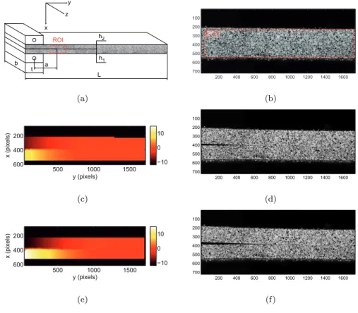
A DCB sample is first analyzed. Its geometry is shown in Figure 2(a). The corresponding dimensions are b = 20 mm, h1 = 2.15 mm, h2 = 1.85 mm,
L = 250 mm, and t = 20 mm. All the plies are aligned along the 0◦-degree
direction (or y-axis, see Figure 2(a)) perpendicular to the loading direction (i.e., x-axis), and there is a pre-crack of length a0 at the separation plane. The
sample was loaded under a displacement controlled procedure. In the following, the end of the loading step will be analyzed.
Figure 2 about here
Figure 2 shows three pictures of the experiment, namely, the reference one and two of the surface in its deformed configuration. They are used to measure displacements via Q4-DIC [25] in which the displacement field is based upon a finite element discretization with 4-noded bilinear (Q4) elements. The com-mercial code CorreliSTCr was used [33]. In the present case, the size of each
element edge is equal to 16 pixels (or ≈ 200 µm). The corresponding transverse displacement fields are shown. The presence of the crack is clearly seen on both pictures and on the displacement fields themselves.
2.2. CLS configurations
The modified Cracked Lap Shear (CLS) or mode II test configuration is shown in Figure 3(a). It consists in a tensile-like specimen made of plies aligned along the 0◦-direction with respect to the loading direction. The dimensions
are b = 10 mm, h1= 1.6 mm, h2 = 1.9 mm, L = 350 mm with a pre-crack of
length a0 at the separation plane. In such conditions, a longitudinal
displace-ment applied on one arm in conjunction with a clamped condition at the other end of the specimen leads to a mixed crack propagation mode. Two lateral confinements (in the x-direction, see Figure 3(a)) are put into contact with the external surfaces in order to avoid opening and as a consequence prevent any mode I contributions (as will be shown hereafter, the loads introduced by the grips are of second order of magnitude with respect to the longitudinal loads).
Figure 3 about here
This geometry has several advantages. First, it enables for the use of the same device for static and dynamic tests to ensure that comparisons are made on the same basis in a quasi pure mode II. Second, the propagation is confined to a longitudinal domain. The determination of the loading possibly transmitted to the specimen does not involve any complex analysis. A first order estimate of the critical value Gc of the energy release rate is determined by using a classical
beam solution for a steady state value [4]
Gc=
F2 ch2
2E1b2h1(h1+ h2)
(1)
where Fc is the maximum load level, b the width of the sample, and E1 the
Young’s modulus in the longitudinal direction.
A first propagation is sought in a displacement controlled manner. The main difficulty of this type of experiment is then related to the location of the crack
tip. This task is performed by resorting to Q4-DIC [25]. The size of each ele-ment edge is equal to 32 pixels (or ≈ 200 µm) ; it is chosen since it corresponds to a good compromise between uncertainty level and spatial resolution. As soon as the first propagation occurs, the sample is unloaded, and then subsequently loaded up to a level of 5 kN. The crack is maintained open and the camera is moved until the crack tip is located at about the center of the picture. Fig-ure 3(b) shows a displacement field in which the presence of a crack is clearly distinguished. The exact position of the crack tip is still unknown. It will be determined more precisely in the sequel.
After the crack is detected in the picture, four additional pictures are shot every 1 kN. For a load level of 9.6 kN, unstable (or undetermined) crack prop-agation occurred. No additional pictures are taken. The CLS configuration is theoretically quasi-unstable since the first derivative of G with respect to the crack length is equal to 0 (see Equation (1)). The analysis of this experiment consists of the five displacement fields corresponding to load levels ranging from 5 to 9 kN.
In the second experiment, no lateral confinement (i.e., no grips) is applied and the mode mixity is induced by the experimental configuration itself. The dimensions of the sample are b = 10 mm, h1= 1.61 mm, h2= 1.57 mm, and L =
250 mm. Two different steps are analyzed. First, the initiation of propagation of the pre-crack close to the groove of the CLS sample is studied. Thirteen loading steps are analyzed. The subsequent propagation was not monitored, but the crack did not cross the whole sample. The next task is then to determine a rough estimate of the crack tip position so that the camera can be moved. The sample is then reloaded (20 loading steps are available) and the beginning of the new propagation step is followed (with 11 pictures). One key issue of this experiment is related to the actual mode mixity and its change during the various loading steps.
3. Identification procedure of fracture mechanics parameters
The following analyses are based upon measured displacement fields umeas
by resorting to Q4-DIC (e.g., Figures 2 and 3). This is the only experimental information that will be used herein. By prescribing the displacements of the external boundary of the region of interest (ROI, see Figure 4(a)) to a finite element calculation of the same part (Figure 4(b)), the way the external load is applied to the crack is accounted for. There is therefore no need to model the whole experiment, but only the part inside the ROI [16]. The computed dis-placements ucompof all inner nodes are used to determine the crack tip position
xc, the first unknown of the fracture mechanics problem. In the present study,
a simple definition of the crack tip location is considered. It corresponds to the location for which the identification error between the measured and computed displacement field is the smallest. It can be noted that other approaches might have been considered (e.g., damage mechanics, cohesive zone model) for which the existence of a crack tip is not necessarily needed. The identification error
δ2(x c) = 1 nm nm X m=1 kumeas(xm) − ucomp(xm, xc)k2 (2)
is minimized with respect to xc, where nmis the number of measurement nodes
located at xm. Various crack positions are considered along the crack surface
di-rection. Each node of the interface is scanned to define a crack tip (Figure 4(b)), and the best position corresponds to the minimum value of the displacement residual δ (Figure 4(c); it corresponds to the 56-th node number in that case).
Figure 4 about here
In the finite element analyses reported hereafter, the behavior of the com-posite is assumed to be elastic. The elastic properties of the two 0-degree lam-inates are as follows, E1 = 120 GPa, G12 = 5.3 GPa, E2 = E33 = 8.9 GPa,
transverse direction is 2, and the out-of-plane one 3. These values were deter-mined in another identification process by performing a series of tensile tests on [0◦], [± 45◦], [± 67.5◦] configurations with loading and unloading sequences [1].
The mesh used in the simulations is refined in comparison with the measure-ment discretization to achieve a finer resolution for the detection of the crack tip. All the points of Q4-DIC are part of the simulation. Consequently, the differences are still performed on the common nodes of the two meshes so that the error is evaluated with respect to the same number of nodes, irrespective of the discretization used. A refinement index ρ is defined such that the number of numerical elements is equal to ρ2 times that of the measurement elements.
The sensitivity of the identification results to the discretization will be studied hereafter. It is worth noting that this refinement is possible thanks to the Q4 interpolation so that no interpolation error on the correlation results is added.
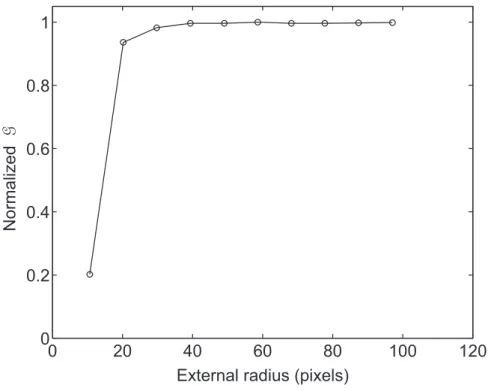
The crack tip position being found (Figure 4(d)), the computed displacement field is post-processed by using fracture mechanics tools available in the finite element code. In the present case, the energy release rate G and the stress intensity factors (SIFs) are evaluated in orthotropic media [34] by using contour integrals [35]. A sensitivity analysis to the size of the integration domain is performed to check that the results have reached a value that becomes domain-independent as expected from a J-integral [36] or an interaction integral [37]. Figure 5 shows the change of G with the external radius of the integration domain. When the radius is greater than 32 pixels the evaluation is virtually insensitive to the size of the integration domain, namely, a fluctuation less than 0.5 % is observed. This minimum radius is equal to the element size of the DIC analysis. This result shows that the minimum size of the integration domain is equal to two elements. In all the analyses that will follow, it was checked that G-values are in a region where the results are independent of the size of the integration domain.
Figure 5 about here
4. Analysis of the three different tests
The various (linear elastic) fracture mechanics parameters are extracted by following the previous procedure for the three tests introduced above.
4.1. DCB experiment
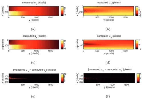
The DCB experiment allows for analyses in which propagation is stable under a displacement controlled test. A series of 28 pictures is considered in addition to the reference picture. One of the aims of the present analysis is to determine which pictures correspond to a situation where propagation does not occur. Further, if propagation occurs, is it under constant G-value? Figure 6 shows a comparison between the measured and computed displacement fields for one of the highest load levels of the series. The residual map is also shown to evaluate the quality of the identification. Except in the immediate vicinity of the crack surface, the residuals are very small (i.e., less than 0.5 pixel or 6 µm). This is to be expected since a Q4-DIC analysis is performed without any discontinuous kinematic enrichment.
Figure 6 about here
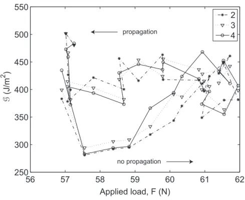
Figure 7 shows the change of the identification error δ as a function of the applied load for three different discretizations. The identification error is inde-pendent of the discretization level when ρ ≥ 2. The case ρ = 1 leads to results different from the reported ones. Two regimes are observed. First, when the crack does not propagate (and the load level increases), the identification error is of the order of 0.2 pixel (or 2.4 µm). This value is larger than the standard displacement uncertainty (of the order of 0.04 pixel or 0.5 µm). It is explained by the fact that a purely elastic model is only a first order approximation of the
interfacial and intralaminar behavior. Second, when the crack propagates (and the load level decreases), there is a gradual increase of the identification error. The last points are likely to be less well tuned. One reason is that the crack tip moves closer to the edge of the region of interest and less measurement points exist in the ligament so that the evaluation of the energy release rate is less accurate.
Figure 7 about here
The location of the crack tip as a function of the load level is shown in Figure 8. Three different refinements are used. The root mean square (RMS) difference between these three results is less than 5 pixels (i.e., 60 µm). A very small effect of the discretization is observed. When analyzing the first 12 points (for which the load level increases), it is seen that the standard uncertainty of the crack tip location is of the order of 14 pixels (or 170 µm). For the last 16 points (for which the load level decreases), there is a clear motion of the crack tip. When a linear interpolation is used, the level of fluctuations is equal to 10 pixels (i.e., 120 µm), which is close to the previous value. It is therefore believed that the local fluctuations are an indication of the identification uncertainty rather than of physical origin. When compared to classical methods where a visual inspection of the crack size is performed (i.e., with a ± 500 µm resolution), there is a clear benefit of using the approach developed herein, which is mechanically-based.
Figure 8 about here
Figure 9 shows the change of the energy release rate G with the applied load for the 28 analyzed pictures. The RMS difference between the three refinements is equal to 15 J/m2. This low value is consistent with the previous results in
trends when the first 12 points are considered in comparison with the last 16 ones. This difference is related to the fact that propagation has occurred for the latter ones. In the first part, a parabolic interpolation leads to a RMS error of about 50 J/m2, as well as with a constant level for the second part (for which
Gc= 410 ± 50 J/m2).
Figure 9 about here
To analyze further the effect of the crack tip location, the first nine points for which the load variation is less than 5 N are considered. The evaluation of G performed before is compared with that obtained with a constant crack tip loca-tion. Figure 10 shows the correlation obtained when comparing these two ways of identifying G values. The RMS difference is of the order of 50 J/m2. These
levels of uncertainty are in accordance with those obtained by a classical global method [3] based on load measurements. This level proves that the fluctuations observed in G-values are related to the uncertainty of crack tip position. There-fore it is believed that the fluctuations observed during the propagation stage are essentially related to measurement and identification uncertainties, and not to physical phenomena due to, say, local variations in interfacial properties, which are known to remain small in the present configuration.
Figure 10 about here
Last, the mode mixity is studied during the two steps of cracking. The fact that the two beam thicknesses are slightly different may induce some mixity. The ratio GI/GII reaches high values, on average equal to 17. This value is virtually
independent of the refinement index, and therefore assumed to be physical. The mixity remains of the same order of magnitude prior to and during the propagation step, with a negligible part of mode II contribution (i.e., 27 J/m2
on average). The DCB test is therefore not only mode I dominant, but purely mode I in the present configuration.
4.2. CLS experiments
4.2.1. Modified CLS experiment
In the modified CLS experiment reported herein, propagation is mainly un-stable and the analysis is restricted to the 5 load levels for which pictures were shot. An additional information is given by the maximum load Fcthat the
sam-ple could sustain after the series of pictures was taken (Fc= 9.6 kN). With that
information, the critical value Gcis determined by using Equation (1). With the
material parameters given above, Gc= 1320 J/m2. This value will be compared
with those obtained by analyzing the 5 load levels with the above-described procedure.
Figure 11 shows a comparison between the measured and computed dis-placement fields for the 9 kN load level. The residual map is also shown to evaluate the quality of the identification. An identification error of 0.3 pixel (or 1.8 µm) is found. This value is small in terms of physical quantity, how-ever larger than the measurement uncertainty evaluated to be of the order of 0.05 pixel (or 0.3 µm). When analyzing the residual maps (Figure 11(e,f)), the maximum values are for the elements cut by the crack in the measured data. This is to be expected since a Q4-DIC analysis was performed without any dis-continuous kinematic enrichment. When this zone is left out for the evaluation of the residuals, the identification error decreases to 0.25 pixel (or 1.5 µm). The same trend is observed for the four analyzed cases.
Figure 11 about here
In the following analysis, the mesh used in the simulations is again refined in comparison with the measurement discretization. Figure 12(a) shows the change of G with the applied load for different values of ρ. The results are weakly dependent on the discretization when ρ ≥ 2. The results with ρ = 1 are completely different from those reported in Figure 12(a) and are not shown. An
overall standard deviation less than 20 J/m2 is observed, which is acceptable
and in line with classical deviations reached with global identification methods. Figure 12(b) shows the mean values obtained with the five analyzed load levels, and the one obtained from the knowledge of the maximum load level (hexagram). If the results of the five load levels were extrapolated to the maximum load, they would reach a value of the order of 1250-1350 J/m2, in good agreement with
the value found previously (i.e., 1320 J/m2).
Figure 12 about here
In terms of identification residuals, Figure 13 shows the change of the identi-fication error δ as a function of the applied load. The range of δ varies between 0.15 and 0.25 pixel (or 0.9 − 1.5 µm). There is a clear degradation when the applied load level increases. The fact that the order of magnitude of the error remains the same indicates that the overall quality of identification does not change. These levels show that even though the agreement between measured and identified fields is good, a purely elastic description of the behavior of the interface and the plies is only a first order approximation of the true one. Last, the influence of the discretization is weak on the overall identification quality when ρ > 1. This trend is to be expected by analyzing the results shown in Figure 12(a). The case ρ = 1 leads to residuals that are systematically higher than those observed for ρ ≥ 1. There is therefore a clear benefit in using a more refined FE mesh. However, a very fine mesh is not needed since the results are virtually mesh-independent as soon as ρ ≥ 2.
Figure 13 about here
The location of the crack tip as a function of the load level is shown in Figure 14. It is worth noting that the crack tip location is directly related to the underlying finite element mesh, namely, each node along the crack path is
considered (Figure 4). For the first three load levels, there is a ± 20 pixel (or ± 120 µm, which is in all cases more accurate than any visual inspection used in classical methods) difference in the location of the crack tip when different meshes are used. Conversely, for the last two load levels, all results are virtually identical for ρ greater than 3. Larger values of ρ allow for a better spatial resolution of the crack tip position. The fact that the crack tip moves as the load level is increased is related to its opening that becomes more easily quantified and identified.
Figure 14 about here
The mode mixity is finally addressed. The point of using lateral confinement was to minimize the mode I contribution. The ratio GI/GIIwill thus be analyzed
for the two CLS configurations studied herein. Figure 15 shows the change of GI/GII with the applied load for the five different mesh densities. Contrary to
what is observed for G and the crack tip position, the ratio GI/GII fluctuates
more due to small variations in GI (± 20 J/m2) for levels varying between 20
and 60 J/m2. For the highest load level, the mean G
I/GII ratio is equal to 0.12
for the five discretizations. Even though there are fluctuations with the applied load, the mode mixity remains low during the load history. It is in accordance with a mode II dominant configuration and below the classical value without confinement, i.e., a mean ratio of about 0.20 is classically reported [38, 39]. The difficulty to set up the confinement supports and the local extraction (instead of global one) are explanations to this difference. The main point is that the present method captures all mode mixity effects whatever the condition and configuration of the actual test.
4.2.2. Standard CLS experiment
To compare the mode mixity observed in the previous configuration, a stan-dard CLS experiment is also performed. In all the analyses to follow, a value of the refinement index ρ = 2 is chosen. Two different phases are analyzed. The initiation of the first crack, which is always delicate since it depends on the sam-ple preparation and in particular on the details of the bonding state close to the teflon tape. Because propagation may be very quickly unstable, this first step is critical in CLS experiments as shown above. Figure 16 shows the change of G with the applied load. The dashed line shows that a quadratic interpolation is a very good approximation of the G vs. applied load curve. The RMS difference between the predicted and measured values is less than 70 J/m2. This value is
close to the estimated uncertainty of G values (i.e., 50 J/m2), thereby indicating
that a quadratic interpolation is a good estimate of the dependence of G with the applied load.
Figure 16 about here
With the same material parameters as above, the application of Equation (1) leads to Gc = 1260 J/m2 for the maximum applied load (Fc = 9.9 kN). This
value is significantly lower than what is identified with the proposed approach (i.e., Gc = 2100 J/m2, see Figure 16). It is worth remembering that an initial
crack is not necessarily present and therefore the applicability of Equation (1) is not guaranteed (i.e., no steady state propagation is observed). The fact that a very high initiation value is found explains why the observation of subsequent propagation is very difficult in this type of test. Since a lot of elastic energy is stored prior to propagation, it may be sufficient to induce a very significant propagation before the crack stops.
One key information in CLS experiments and for the present identification method is related to the mode mixity. Figure 17 shows the change of the ratio
GI/GII with the applied load. The ratio remains less than 0.08 throughout
the whole loading sequence for which no propagation occurs. It is therefore concluded that the initiation stage is mainly mode II controlled. However, the initial loading does not proceed with a constant mode mixity. Close to the maximum load level for which a picture is recorded, the initiation itself is mode II dominant. The fluctuations of mode mixity may explain part of the difference observed in terms of dependence of G with the applied load. For orthotropic media, a complex coupling appears between GI and GII that does not lead to a
linear dependence (classically known for isotropic media) [34].
Figure 17 about here
This is confirmed by analyzing the changes of the two SIFs with the applied load (Figure 18). The mode II SIF follows a linear dependence with the applied load whereas the mode I SIF fluctuates during the whole loading history. These fluctuations, which are very difficult to control experimentally, are responsible for the small variations around a quadratic response of G. Last, when com-pared with the previous CLS configuration, it is observed that the GI/GII ratio
becomes even smaller without any lateral confinement.
Figure 18 about here
Even though a very high value of G is observed in the initiation stage (Fig-ure 16), the crack does not traverse the whole sample. It stops at about the middle length of the beam. The displacement is then decreased to a very small value. After roughly locating the crack tip by visually analyzing the displace-ment maps provided by Q4-DIC, the applied displacedisplace-ment is increased again. In the present case, it is possible to follow the beginning of propagation until the crack tip is no longer located in the picture. Figure 19 shows the change of G with the applied load during the two stages (i.e., no propagation and
sub-sequent propagation). The first stage leads to a quasi quadratic G vs. applied load trend as previously observed.
Figure 19 about here
The deviation from the quadratic response is again due to the value of mode I SIF that varies significantly during the first loading part. It leads to very high values of mode mixity (Figure 20) especially at the beginning of the load-ing history. This may be due to loadload-ing conditions that are not strictly those associated with a CLS geometry due to small misalignments. It is worth remem-bering that this type of analysis is only possible when these various quantities are extracted with the true experimental conditions (i.e., the displacements on the boundary of the ROI).
Figure 20 about here
During propagation, there is a clear increase of G as the load level decreases (see inset of Figure 19). An interpolation by the inverse of the applied load captures the trend observed experimentally. Contrary to the first part of the loading history, this second part is characterized by a slight increase of mode mixity GI/GII from 0.09 to 0.12 (Figure 20). The value at the onset of
prop-agation is below the mean estimate without confinement (i.e., 0.20 [38, 39]) and is below the ratio obtained with confinement. The difficulty to set up the lateral confinements is again pointed out. In spite of this complex preparation, the present local extraction gives good tendencies and more accurate estimates than only from a classical (global) analysis, which does not give access to actual (and varying) mode mixities.
When compared with the modified CLS configuration, the same level of GI/GII ratio is observed. The effect of lateral confinement is therefore minimal
deviation from the value as propagation proceeds. This result proves that prop-agation is not under a constant mode mixity and that the present method is able to capture it. The fact Gc increases with the crack length may be due to
an R-curve behavior since an increase of the mode mixity cannot explain the increase in toughness (since these materials are classically known to have Gc
-values that are significantly higher under mode II propagation compared with mode I propagation [40]).
Last, with the material parameters given above, Jc = 860 J/m2 for the
maximum applied load (Fc = 8.3 kN). This value is of the same order of
mag-nitude, yet lower than what is identified during the propagation stage (i.e., Gc= 670 − 730 J/m2, see inset of Figure 19). This trend is identical for all the
cases studied herein.
4.3. Discussion
In the present analyses, the location of the crack tip was shown to be more accurate (i.e., ± 120 µm) than classical (visual) procedures (of the order of ± 500 µm), which are operator-dependent since it is performed by analyzing pictures of the edge of the sample. The standard uncertainty in G values was shown to be at most equal to 50 J/m2, which is significant but acceptable, for
DCB tests for which a critical value of G is of the order of 400 J/m2. Conversely,
for the CLS test values as high as 1300 J/m2are determined, and even greater
than 2000 J/m2 at initiation. Thanks to the sub-pixel resolution of Q4-DIC,
this new methodology, which is encapsulated in a unique tool, offers a safer and more robust evaluation compared with global and visual techniques.
The analysis of mode mixity shows that it can sometimes deviate quite sig-nificantly from the theoretical estimates based upon ideal loading conditions. The evaluation of the true boundary conditions was crucial to draw this type of conclusion. In particular, it is shown that passive (i.e., lateral) confinements
have to be controlled in a very complex manner to ensure the quasi-pure mode II configuration for CLS configurations. One of the reasons being the Poisson contraction associated with the tensile load. For DCB experiments, when the two heights of the beams are not identical, small mode II contributions are ob-served. For all geometries and configurations, the mode mixity extracted at the local scale is more accurate than (former) global extractions since experimen-tal boundary conditions are continuously accounted for during the propagation events.
5. Conclusions
In this paper, three tests were analyzed to determine critical propagation parameters in mode I and II conditions, and also a mixed mode I/II configura-tion by extension. This is achieved by coupling displacements fields measured by resorting to digital image correlation and finite element simulations. The common information is given by the measured displacements on the boundary of the region of interest that are the boundary conditions of the finite element simulations. By minimizing the distance between the measured and computed displacement fields, it is possible to determine the crack tip location. The latter being determined, energy release rates associated with each mode are evaluated by post-processing the finite element results. The experimental mode mixity is also accessible by following the procedure proposed herein for any of the ana-lyzed geometries and configuration.
These encouraging results show that the identification of more advanced (cohesive) models of any interface parameters (e.g., the stiffness of the interface) can be reached without any global sensor measurement, the two layers can be seen as a “stress gauge,” provided their elastic properties are known and no intralaminar damage develops during the test. (Nonlinear contributions of the intralaminar behavior may also be accounted for in the present setting.)
Local kinematic fields may also be used to identify propagation parameters under more complex configurations (e.g., interfaces between [± θ] plies) since the approach developed herein is very generic, and does not rest on closed-form solutions whose applicability is restricted to very simple cases. It also shows that it is possible to extract directly intrinsic propagation parameters (e.g., GIc and GIIc), but also initiation values and a direct evaluation of the mode
mixity even when it is not constant during the whole test. These emerging identification methods fully support the virtual testing approach in the way to reduce numerous classical tests with a poor quality of parameter extraction to the benefit of new identification methods with added value [41, 42, 43, 44]. They can also be used as a redundant check of any identification process or for local counter-expertise of any complex delamination process.
Acknowledgements
The support of this research by “Agence Nationale pour la Recherche” is gratefully acknowledged (VULCOMP Phase 1 project, grant number ANR-2006-MAPR-0022-01).
References
[1] Ladev`eze P, Le Dantec E. Damage modelling of the elementary ply for laminated composites. Comp Sci Tech. 1992;43(3):257-67.
[2] Allix O, Blanchard L. Mesomodeling of delamination: towards industrial applications. Comp Sci Tech. 2006;66(6):731-44.
[3] ASTM D5528 - 01e3 Standard Test Method for Mode I Interlaminar Frac-ture Toughness of Unidirectional Fiber-Reinforced Polymer Matrix Com-posites. West Conshohocken, PA (USA): ASTM; 2007.
[4] ASTM D5868 - 01 Standard Test Method for Lap Shear Adhesion for Fiber Reinforced Plastic (FRP) Bonding. West Conshohocken, PA (USA): ASTM; 2008.
[5] Allix O, Corigliano A. Modeling and simulation of crack propagation in mixed-modes interlaminar fracture specimens. Int J Fract. 1996;77:111-40.
[6] Derewonko A, Godzimirski J, Kosiuczenko K, Niezgoda T, Kiczko A. Strength assessment of adhesive-bonded joints. Comput Mat Sci. 2008;43(1):157-64.
[7] Kanninen MF, Popelar CH. Advanced Fracture Mechanics. Oxford (UK): Oxford University Press; 1985.
[8] Pardoen T, Ferracin T, Landis CM, Delannay F. Constraint effects in ad-hesive joint fracture. J Mech Phys Solids. 2005;53:1951-83.
[9] Leffler K, Alfredsson KS, Stigh U. Shear behaviour of adhesive layers. Int J Solids Struct. 2007;44:530-45.
[10] Sørensen BF, Gamstedt EK, Østergaard RC, Goutianos S. Micromechani-cal model of cross-over fibre bridging - Prediction of mixed mode bridging laws. Mech Mat. 2008;40:220-34.
[11] Salomonsson K, Andersson T. Modeling and parameter calibration of an adhesive layer at the meso level. Mech Mat. 2008;40(1-2):48-65.
[12] Yang QD, Thouless MD, Ward SM. Elastic-plastic mode-II fracture of ad-hesive joints. Int J Solids Struct. 2001;38:3251-62.
[13] Su C, Wei YJ, Anand L. An elastic-plastic interface constitutive model: Application to adhesive joints. Int J Plasticity. 2004;20:2063-81.
[14] Sargent JP. Durability studies for aerospace applications using peel and wedge tests. Int J Adhesion Adhesives. 2005;25:247-56
[15] Abanto-Bueno J, Lambros J. Investigation of crack growth in function-ally graded materials using digital image correlation. Eng Fract Mech. 2002;69:1695-711.
[16] Fedele R, Raka B, Hild F, Roux S. Identification of adhesive properties in GLARE assemblies by Digital Image Correlation. J Mech Phys Solids. 2009;57:1003-16.
[17] Ireman T, Thesken JC, Greenhalgh E, Sharp R, G¨adke M, Maison S, et al. Damage propagation in composite structural elements-coupon experiments and analyses. Comp Struct. 1996;36:209-20.
[18] IGC 4.26.381. Instruction g´en´erale de contrˆole pour la d´etermination du G1c. A´erospatiale standard (in French); 1991.
[19] AITM 1.0005. Determination of interlaminar fracture toughness energy. Airbus Industrie Test Method, Issue 2; 1994.
[20] Sutton MA, McNeill SR, Helm JD, Chao YJ. Advances in Two-Dimensional and Three-Dimensional Computer Vision. In: Rastogi PK, editor. Pho-tomechanics. Berlin (Germany): Springer; 2000. p. 323-72.
[21] Sutton MA, Zhao W, McNeill SR, Helm JD, Piascik RS, Riddel WT. Local crack closure measurements: Development of a measurement system using computer vision and a far-field microscope. In: McClung RC, Newman Jr. JC, editors. Advances in fatigue crack closure measurement and analysis: second volume, STP 1343: ASTM; 1999. p. 145-56.
[22] Chasiotis I, Knauss WG. A New Microtensile Tester for the Study of MEMS Materials with the Aid of Atomic Force Microscopy. Exp Mech. 2002;42(1):51-7.
[23] Forquin P, Rota L, Charles Y, Hild F. A Method to Determine the Tough-ness Scatter of Brittle Materials. Int J Fract. 2004;125(1):171-87.
[24] Chasiotis (edt.) I. Special issue on nanoscale measurements in Mechanics. Exp Mech. 2007;47(1).
[25] Besnard G, Hild F, Roux S. “Finite-element” displacement fields analy-sis from digital images: Application to Portevin-Le Chˆatelier bands. Exp Mech. 2006;46:789-803.
[26] McNeill SR, Peters WH, Sutton MA. Estimation of stress intensity factor by digital image correlation. Eng Fract Mech. 1987;28(1):101-12.
[27] Geers MGD, De Borst R, Peijs T. Mixed numerical-experimental identi-fication of non-local characteristics of random-fibre-reinforced composites. Comp Sci Tech. 1999;59:1569-78.
[28] Cho S, C´ardenas-Garc´ıa JF, Chasiotis I. Measurement of Nanodisplace-ments and Elastic Properties of MEMS via the Microscopic Hole Method. Sensors and Actuators A. 2005;120:163-71.
[29] Maier G, Bocciarelli M, Fedele R. Some innovative industrial prospects cen-tered on inverse analyses. In: Mr´oz Z, Stavroulakis G, editors. Parameter
Identification of Materials and Structures CISM Lecture Notes: Springer Verlag, Wien; 2005. p. 47-73.
[30] Hild F, Roux S. Digital image correlation: From measurement to identifi-cation of elastic properties - A review. Strain. 2006;42:69-80.
[31] Abanto-Bueno J, Lambros J. Experimental Determination of Cohe-sive Failure Properties of a Photodegradable Copolymer. Exp Mech. 2005;45(2):144-52.
[32] Simulia. Abaqus Analysis User’s Manual (version 6.7) 2010.
[33] http://www.holo3.com/correli-stcr-afr17.html
[34] Sih GC, Paris PC, Irwin GR. On cracks in rectilinearly anisotropic bodies. Int J Fract Mech. 1965;1:189-203.
[35] Simulia. Contour integral evaluation (section 11.4.2). Abaqus Analysis User’s Manual (version 6.7) 2010. See also Stress intensity factor extraction (section 2.16.2). Abaqus Theory Manual (version 6.7) 2010.
[36] Rice JR. A Path Independent Integral and Approximate Analysis of Strain Concentrations by Notches and Cracks. ASME J Appl Mech. 1968;35:379-86.
[37] Parks DM. A stiffness derivative finite element technique for determination of crack tip stress intensity factors. Int J Fract. 1974;10(4):487-502.
[38] Russel AJ, Street KN. Moisture and temperature effects on the mixed-mode delamination fracture of unidirectional graphite epoxy. Delamination and debonding of materials: ASTM , Philadelphia (PA), USA; 1985. p. 349-70.
[39] Rhee KY. Characterization of delamination behavior of unidirectional graphite/PEEK laminates using cracked lap shear (CLS) specimens. Comp Struct. 1994;29:379-82.
[40] L´evˆeque D. Analyse de la tenue au d´elaminage des composites stratifi´es : identification d’un mod`ele d’interface interlaminaire [PhD thesis]: ENS Cachan; 1998.
[41] Ben Azzouna M, P´eri´e J-N, Guimard J-M, Hild F, Roux S. On the identi-fication and validation of an anisotropic damage model by using full-field measurements. Int J Damage Mech. 2011;20(8):1130-50.
[42] Cox B, Yang Q. In Quest of Virtual Tests for Structural Composites. Sci-ence. 2006;314:1102-7.
[43] Gonz´alez C, LLorca J. Virtual fracture testing of composites: A computa-tional micromechanics approach. Eng Fract Mech 2007;74:1126-38.
[44] Davies GOA, Ankersen J. Virtual testing of realistic aerospace composite structures. J Mat Sci 2008;42(20):6586-92.
List of Figures
1 Different identification methods for the toughness of a DCB test from the applied load versus stroke curve. AITM method: one mean value is extracted from all the experimental data. IGC method: one value per cycle is determined. In the method devel-oped herein each picture pair can be used to evaluate the current energy release rates and mode mixities . . . 30 2 (a): DCB sample and location of the Region of Interest to analyze
locally the displacement field in the vicinity of the crack tip. (b): Reference picture of the experiment. (c,e): Vertical displacement fields (in pixels) from which the rigid body motions have been subtracted (1 pixel ↔ 12 µm). 16-pixel Q4 elements are used in the DIC analysis. (d,f): Corresponding pictures in the deformed configuration . . . 31 3 (a): CLS sample and location of the Region of Interest to analyze
locally the displacement field in the vicinity of the crack tip. (b): Horizontal displacement field (in pixels) from which the rigid body motions have been subtracted (1 pixel ↔ 6 µm). 32-pixel Q4 elements are used in the DIC analysis . . . 32 4 Different steps for the determination of the crack tip position . . 33 5 J-integral normalized by its maximum value as a function of the
external radius of the integration domain. For an external radius greater than 32 pixels, the evaluation of J = G is independent of its value . . . 34 6 (a,b): Measured, (c,d): computed, and (e,f): residual
displace-ment fields in the vertical (left) and horizontal (right) directions (1 pixel ↔ 12 µm) for the DCB experiment . . . 35
7 Change of the identification error δ with the refinement index ρ for the 28 load levels of the DCB experiment (1 pixel ↔ 12 µm). The first part corresponds to a load increase with no propagation, and the second part is associated with a load decrease during crack propagation . . . 36 8 Crack tip position as a function of the applied load level for three
different refinement indices ρ for the DCB experiment (1 pixel ↔ 12 µm). The first part corresponds to a load increase with no propagation, and the second part is associated with a load decrease during crack propagation . . . 37 9 G as a function of the applied load level for the three refinement
indices ρ for the DCB experiment. The first part corresponds to a load increase with no propagation, and the second part is associated with a load decrease during crack propagation . . . . 38 10 Sensitivity of G with respect to the crack tip position.
Com-parison of G determined for a fixed crack tip position (Gf) as a
function G determined for a variable crack tip position (Gv, see
Figure 9) for the DCB experiment. The dashed line corresponds to a linear interpolation of slope equal to 1. The RMS difference between the two estimates is of the order of 50 J/m2 . . . . 39
11 (a,b): Measured, (c,d): computed and (e,f): residual displace-ment fields in the horizontal (left) and vertical (right) directions for the 9 kN load level of the modified CLS experiment (1 pixel ↔ 6 µm) . . . 40
12 -a-Change of G with the refinement index ρ for the five load levels (CLS experiment). A 16 J/m2 RMS difference is observed when
the different results are compared. -b-Average G as a function of the applied load. The hexagram corresponds to the evaluation of the critical value by using Equation (1) . . . 41 13 Change of the identification error with the refinement index ρ
for the five load levels of the modified CLS experiment (1 pixel ↔ 6 µm) . . . 42 14 Crack tip position as a function of the applied load level for five
refinement indices ρ for the modified CLS experiment (1 pixel ↔ 6 µm) . . . 43 15 Energy release rate ratio as a function of the applied load level
for the modified CLS experiment . . . 44 16 G as a function of the applied load level for the initiation step of
the CLS experiment. The dashed line corresponds to a parabolic interpolation . . . 45 17 GI/GII ratio as a function of the applied load level for the
initi-ation step of the CLS experiment . . . 46 18 Mode I and II SIFs as functions of the applied load level for the
initiation step of the CLS experiment. The dashed line corre-sponds to a linear interpolation . . . 47 19 G as a function of the applied load level for the propagation step of
the CLS experiment. The dashed line corresponds to a parabolic interpolation. Inset: detail of the propagation history. The solid line corresponds to a hyperbolic interpolation . . . 48 20 GI/GII ratio as a function of the applied load level for the
Stroke
Ap
p
lie
d
l
o
a
d
Experimental data IGC AITMFigure 1: Different identification methods for the toughness of a DCB test from the applied load versus stroke curve. AITM method: one mean value is extracted from all the experimental data. IGC method: one value per cycle is determined. In the method developed herein each picture pair can be used to evaluate the current energy release rates and mode mixities
h2 a L b t ROI h1 x y z (a) 200 400 600 800 1000 1200 1400 1600 100 200 300 400 500 600 700 ROI (b) y (pixels) x (p ixe ls) 500 1000 1500 200 400 600 −10 0 10 (c) 200 400 600 800 1000 1200 1400 1600 100 200 300 400 500 600 700 (d) y (pixels) x (p ixe ls) 500 1000 1500 200 400 600 −10 0 10 (e) 200 400 600 800 1000 1200 1400 1600 100 200 300 400 500 600 700 (f)
Figure 2: (a): DCB sample and location of the Region of Interest to analyze locally the displacement field in the vicinity of the crack tip. (b): Reference picture of the experiment. (c,e): Vertical displacement fields (in pixels) from which the rigid body motions have been subtracted (1 pixel ↔ 12 µm). 16-pixel Q4 elements are used in the DIC analysis. (d,f): Corresponding pictures in the deformed configuration
h
2a
L
b
ROI
x
y
z
h
1 (a)y (pixels)
x
(p
ixe
ls)
200
400
600
800
1000
300
400
500
600
−1
0
1
(b)Figure 3: (a): CLS sample and location of the Region of Interest to analyze locally the displacement field in the vicinity of the crack tip. (b): Horizontal displacement field (in pixels) from which the rigid body motions have been subtracted (1 pixel ↔ 6 µm). 32-pixel Q4 elements are used in the DIC analysis
(a) Deformed mesh determined by Q4-DIC. The measured dis-placements of nodes in red are prescribed in FE analyses. The inner nodes (in blue) are used to minimize the identification er-ror δ
x y
(b) FE mesh in which the interface nodes that are not broken are marked in yellow
40 50 60 70 80 90
3.0 3.2 3.4 3.6
Crack tip position (node number)
Id e n ti fi ca ti o n e rro r (µ m) 3.1 3.3 3.5 3.7
(c) Change of the identification error δ as a function of the assumed position for the crack tip 200 400 600 800 1000 1200 1400 1600 100 200 300 400 500 600 700
(d) Optimal crack tip position marked with white arrow Figure 4: Different steps for the determination of the crack tip position
0
20
40
60
80
100
120
0
0.2
0.4
0.6
0.8
1
External radius (pixels)
N
o
rma
lize
d
G
Figure 5: J-integral normalized by its maximum value as a function of the external radius of the integration domain. For an external radius greater than 32 pixels, the evaluation of J = G is independent of its value
y (pixels) x (p ixe ls) measured u x (pixels) 0 500 1000 1500 0 200 −5 0 5 10 (a) y (pixels) x (p ixe ls) measured u y (pixels) 0 500 1000 1500 0 200 −3 −2 −1 0 1 (b) y (pixels) x (p ixe ls) computed ux (pixels) 0 500 1000 1500 0 200 −5 0 5 10 (c) y (pixels) x (p ixe ls) computed uy (pixels) 0 500 1000 1500 0 200 −2 0 2 (d) y (pixels) x (p ixe ls)
|measured ux − computed ux| (pixels)
500 1000 1500 100 200 300 2 4 6 8 10 (e) y (pixels) x (p ixe ls)
|measured uy − computed uy| (pixels)
500 1000 1500 100 200 300 2 4 (f)
Figure 6: (a,b): Measured, (c,d): computed, and (e,f): residual displacement fields in the vertical (left) and horizontal (right) directions (1 pixel ↔ 12 µm) for the DCB experiment
56
57
58
59
60
61
62
0.15
0.2
0.25
0.3
0.35
0.4
0.45
0.5
0.55
Applied load, F (N)
Id
e
n
ti
fi
ca
ti
o
n
e
rro
r
(p
ixe
l)
2
3
4
no propagation propa gationFigure 7: Change of the identification error δ with the refinement index ρ for the 28 load levels of the DCB experiment (1 pixel ↔ 12 µm). The first part corresponds to a load increase with no propagation, and the second part is associated with a load decrease during crack propagation
56
57
58
59
60
61
62
650
700
750
800
850
900
950
1000
Applied load, F (N)
C
ra
ck
ti
p
co
o
rd
in
a
te
,
x
c(p
ixe
ls)
2
3
4
no propagation pro pagatio nFigure 8: Crack tip position as a function of the applied load level for three different refinement indices ρ for the DCB experiment (1 pixel ↔ 12 µm). The first part corresponds to a load increase with no propagation, and the second part is associated with a load decrease during crack propagation
56
57
58
59
60
61
62
250
300
350
400
450
500
550
Applied load, F (N)
G
(J/
m
2)
2
3
4
no propagation propagationFigure 9: G as a function of the applied load level for the three refinement indices ρ for the DCB experiment. The first part corresponds to a load increase with no propagation, and the second part is associated with a load decrease during crack propagation
250
300
350
400
450
500
280
300
320
340
360
380
400
420
440
460
G
v(J/m
2)
G
f(J/
m
2)
Figure 10: Sensitivity of G with respect to the crack tip position. Comparison of G deter-mined for a fixed crack tip position (Gf) as a function G determined for a variable crack tip
position (Gv, see Figure 9) for the DCB experiment. The dashed line corresponds to a linear
interpolation of slope equal to 1. The RMS difference between the two estimates is of the order of 50 J/m2
y (pixels) x (p ixe ls) measured u x (pixels) 0 200 400 600 800 1000 0 200 400 −10 0 10 (a) y (pixels) x (p ixe ls) measured u y (pixels) 0 200 400 600 800 1000 0 200 400 −5 0 5 (b) y (pixels) x (p ixe ls) computed ux (pixels) 0 200 400 600 800 1000 0 200 400 −10 0 10 (c) y (pixels) x (p ixe ls) computed uy (pixels) 0 200 400 600 800 1000 0 200 400 −5 0 5 (d) y (pixels) x (p ixe ls) |measured u x − computed ux| (pixel) 200 400 600 800 1000 100 200 300 400 0.2 0.4 0.6 0.8 1 1.2 1.4 (e) y (pixels) x (p ixe ls) |measured u y − computed uy| (pixel) 200 400 600 800 1000 100 200 300 400 0.5 1 1.5 (f)
Figure 11: (a,b): Measured, (c,d): computed and (e,f): residual displacement fields in the horizontal (left) and vertical (right) directions for the 9 kN load level of the modified CLS experiment (1 pixel ↔ 6 µm)
0 2 4 6 8 10 0 100 200 300 400 500 600 700 Applied load, F (kN) G (J/ m 2) 2 3 4 5 6 (a) 0 2 4 6 8 10 0 200 400 600 800 1000 1200 1400 Applied load, F (kN) G (J/ m 2 ) (b)
Figure 12: -a-Change of G with the refinement index ρ for the five load levels (CLS experiment). A 16 J/m2RMS difference is observed when the different results are compared. -b-Average G
as a function of the applied load. The hexagram corresponds to the evaluation of the critical value by using Equation (1)
0
2
4
6
8
10
0
0.05
0.1
0.15
0.2
0.25
0.3
Applied load, F (kN)
Id
e
n
ti
fi
ca
ti
o
n
e
rro
r
(p
ixe
l)
1
2
3
4
5
6
Figure 13: Change of the identification error with the refinement index ρ for the five load levels of the modified CLS experiment (1 pixel ↔ 6 µm)
0
2
4
6
8
10
140
160
180
200
220
240
260
280
300
320
Applied load, F (kN)
C
ra
ck
ti
p
co
o
rd
in
a
te
,
x
c(p
ixe
ls)
2
3
4
5
6
Figure 14: Crack tip position as a function of the applied load level for five refinement indices ρ for the modified CLS experiment (1 pixel ↔ 6 µm)
0
2
4
6
8
10
0
0.2
0.4
0.6
0.8
1
G
I/
G
IIApplied load, F (kN)
2
3
4
5
6
Figure 15: Energy release rate ratio as a function of the applied load level for the modified CLS experiment
0
500
1000
1500
2000
2500
0
2
4
6
8
10
G
(
J/
m
2
)
Aplied load (kN)
Figure 16: G as a function of the applied load level for the initiation step of the CLS experi-ment. The dashed line corresponds to a parabolic interpolation
0
2
4
6
8
10
0
0.05
0.1
0.15
0.2
G
I/
G
IIApplied load, F (kN)
Figure 17: GI/GII ratio as a function of the applied load level for the initiation step of the
0
2
4
6
8
10
0
0.2
0.4
0.6
0.8
1
0
2
4
6
8
10
K
IIK
IK
II(M
Pa
.m
0 .5)
K
I(M
Pa
.m
0 .5)
Aplied load (kN)
Figure 18: Mode I and II SIFs as functions of the applied load level for the initiation step of the CLS experiment. The dashed line corresponds to a linear interpolation
0
100
200
300
400
500
600
700
800
0
2
4
6
8
10
G
(
J/
m
2
)
Aplied load (kN)
660 670 680 690 700 710 720 730 7.6 7.7 7.8 7.9 8 8.1 8.2 8.3Figure 19: G as a function of the applied load level for the propagation step of the CLS experiment. The dashed line corresponds to a parabolic interpolation. Inset: detail of the propagation history. The solid line corresponds to a hyperbolic interpolation
0
2
4
6
8
10
0
0.2
0.4
0.6
0.8
1
1.2
1.4
G
I/
G
IIApplied load, F (kN)
Figure 20: GI/GIIratio as a function of the applied load level for the propagation step of the