HAL Id: inserm-00134564
https://www.hal.inserm.fr/inserm-00134564
Submitted on 2 Mar 2007
HAL is a multi-disciplinary open access archive for the deposit and dissemination of sci-entific research documents, whether they are pub-lished or not. The documents may come from teaching and research institutions in France or abroad, or from public or private research centers.
L’archive ouverte pluridisciplinaire HAL, est destinée au dépôt et à la diffusion de documents scientifiques de niveau recherche, publiés ou non, émanant des établissements d’enseignement et de recherche français ou étrangers, des laboratoires publics ou privés.
Global Description of Protein 3D Structures
Alexandre de Brevern, Cristina Benros, Serge Hazout
To cite this version:
Alexandre de Brevern, Cristina Benros, Serge Hazout. Structural Alphabet: From a Local Point of View to a Global Description of Protein 3D Structures. Yan, Peter V. Bioinformatics: New Research, Nova publishers, pp.127-69, 2005. �inserm-00134564�
Structural alphabet
Structural alphabet: from a local point of view to a global
description of protein 3D structures.
Alexandre G. de Brevern *
#, Cristina Benros
#& Serge Hazout
Equipe de Bioinformatique Génomique et Moléculaire (EBGM),
INSERM E03-46, Université Denis DIDEROT-Paris 7, case 7113,
2, place Jussieu, 75251 Paris, France
* Corresponding author:
mailing address: Dr. de Brevern A.G., Equipe de Bioinformatique Génomique et
Moléculaire (EBGM), INSERM E 03-46, Université Denis DIDEROT-Paris 7, case
7113, 2, place Jussieu, 75251 Paris, France
E-mail : debrevern@ebgm.jussieu.fr
Tel: (33) 1 44 27 77 31
Fax: (33) 1 43 26 38 30
Running title: structural alphabet
key words: secondary structure, local folds, Bayesian prediction approach,
structure-sequence relationship, protein structural classes, ab initio.
#
both authors have contributed equally to this work.
Abstract
The study of protein structures’ local conformations has a long history principally based on the analysis of the classical repetitive structures (i.e. α-helix and β-sheet), and also on the characterization of some particular structures in the coil state (e.g. turns). The secondary structures are interesting for describing the global protein fold but miss all the orientations of the connecting regions and so neglect many particularities of the coil state.
In order to take these structural features into account, we have identified a local structural alphabet composed of 16 folding patterns of five consecutive residues, called Protein Blocks (PBs). Conversely to the secondary structures, the PBs are able to approximate every part of the protein structures. These PBs have been used both to describe precisely the 3D protein backbones with an average rmsd of 0.42 Å, and to perform a local structure prediction with a rate of correct prediction of 48.7%.
In this chapter, we present the interest of the Protein Blocks by comparing the secondary structure assignment with the assignment in terms of PBs. We highlight the discrepancies between different secondary structure assignment methods and show some interesting correspondence between particular local folds and the Protein Blocks. Then, we use the Protein Block prediction to classify proteins into the classical structural classes, namely all α, all β and mixed. The prediction rate of theses different classes is good, i.e. 71.5%, with no confusion between all α and all β classes. Finally, we present a new approach named TopKAPi that stands for “Triangular Kohonen Map for Analyzing Proteins”. It enables to classify and analyze proteins
according to their Protein Block frequencies using for this purpose a novel unsupervised clustering method: a triangular self-organizing Kohonen map. This method enables to determine new relationships between local structures and amino acid distributions. This new methodology could be of great interest in proteomics and sequence alignment.
Introduction
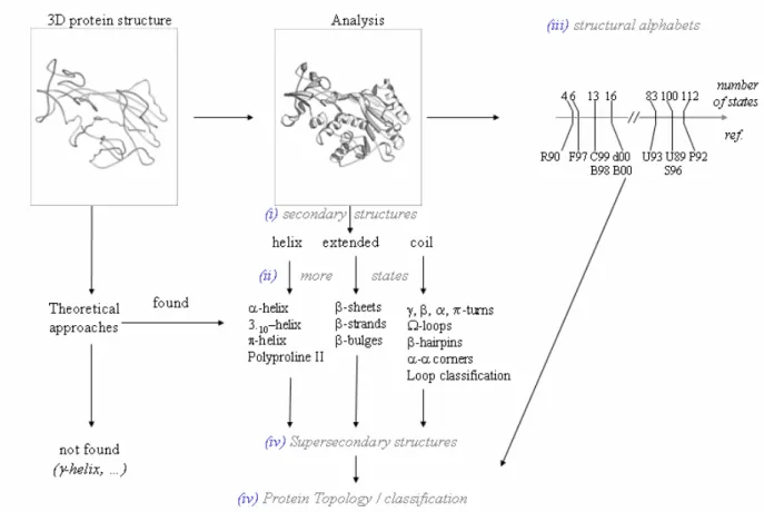
The first protein structure obtained by X-ray diffraction [1] had marked the beginning of the description and analysis of protein structures. Two ways have since been followed with the theoretical methods and the descriptive methods. In the first years, due to the limited number of available structures, the first kind of approaches was used for proposing potential local structures based on physico-chemical properties (e.g. the γ-helix [2]). Their presence and interest in experimentally determined structures were confirmed or not only in a second step [3]. In this chapter, we focus on the second kind of approaches based on the description and characterization of particular local fold structures observed in experimentally determined protein structures. Figure 1 summarizes different levels of description of the protein folds that we are going to follow in this introduction: (i) the 3-states secondary structures, (ii) the secondary structures with more distinct states, (iii) the structural alphabets and (iv) the description of the complete protein topology.
(i) the 3-states secondary structures. One of the major events in the protein history is the
series of seven consecutive papers of Pauling and Corey in 1951. They described an impressive number of potential local folds including the α-helix and the β-sheet [2, 4]. The average
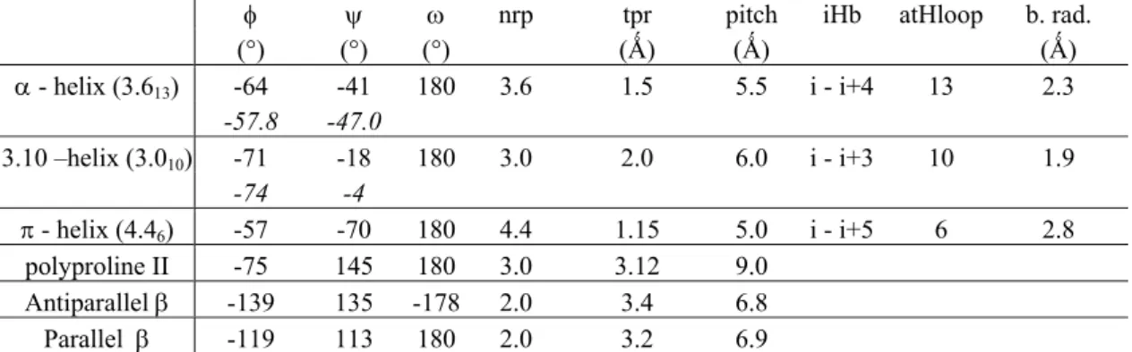
characteristics of these local structures are described in Table 1. The α-helix (or 3.613 helix) is
characterized by intramolecular hydrogen bonds between amino acid residues i and i +4 [5]. Its extremities show specific physicochemical stabilizations [6]. The β-sheet is defined by hydrogen bonds between neighboring parallel (or antiparallel) chains [4]. As for the α-helix, its edges have been widely analyzed [7 - 9]. Many studies have also analyzed the packing of these two repetitive structures [10 - 13] and the sequence - structure relationship between sequence and structure [14 -
17].
Figure 1. Protein structure analysis. From the 3D atom coordinates of a protein structure different analyses are possible. Theoretical approaches consist in predicting potential interesting local structures based on physicochemical criteria. Descriptive approaches are based on the analysis of known local structures at different levels of organization: (i) the secondary structures defined by three states (helicoidal, extended and non-helicoidal /non-extended). (ii) a more detailed description (see Text). Another way to describe the protein structures is by (iii) the use of
structural alphabets that are characterized by different states (references : R90 [125], F97 [126],
C99 [129], B98 [127], d00 [128], B00 [161], U93 [120], U89 [118], S96 [121], P92 [119]). The local folds combinations create local topologies referred to as (iv) super-secondary structures which describe the complete protein topology.
The high propensity of these helicoidal and extented local structures in experimentally determined structures has since achieved one kind of dogma, the ‘secondary structures’ composed of the α-helix, the β-strand and a state corresponding to everything else, the coil. The structures are often limited to this simple description.
φ ψ ω nrp tpr pitch iHb atHloop b. rad. (°) (°) (°) (Ǻ) (Ǻ) (Ǻ) α - helix (3.613) -64 -41 180 3.6 1.5 5.5 i - i+4 13 2.3 -57.8 -47.0 3.10 –helix (3.010) -71 -18 180 3.0 2.0 6.0 i - i+3 10 1.9 -74 -4 π - helix (4.46) -57 -70 180 4.4 1.15 5.0 i - i+5 6 2.8 polyproline II -75 145 180 3.0 3.12 9.0 Antiparallel β -139 135 -178 2.0 3.4 6.8 Parallel β -119 113 180 2.0 3.2 6.9
Table 1. Characterization of classical local folds with their dihedral angles (φ, ϕ and ω, in italics are given the theoretical values), the number of residues per turns (nrp), the translation per residues (tpr), the pitch, the intramolecular hydrogen-bond between (CO, NH) (iHb), the atoms found in the H-bonded loop (atHloop) and the backbone radius.
(ii) the secondary structures with more distinct states. Different studies have examined and
extended these definitions both in creating new states and refining the assignment criteria. They have improved our knowledge of the repetitive helicoidal and extended structures and have highlighted the interest of the coil state too many times badly described as ‘random‘ coil.
The new local folds pointed out exhibit interesting energetic and / or geometrical properties. Thus, less common helices, like 310 – helices are characterized by intramolecular hydrogen
bonds between amino acid residues i and i +3 [18 - 20] and π-helices (i.e. 4.46-helices) with
hydrogen bonds between amino acid residues i and i +5 [21 - 25]. These two types of helicoidal structures are often encountered at the extremities of longer α-helices and seem to play an important role in the stabilization of longer helicoidal structures [26]. The π-bulges constitute a particular kind of discontinuity in helicoidal structures. Like the π-helices, they are not frequent but seem directly associated to protein functions [23, 27]. The Polyproline II helices correspond to a specific local fold initially found in fibrous proteins [28, 29]. They contribute to the creation of coiled coil supersecondary structures characteristic of these proteins. They are also found in globular proteins and are not composed only of Proline [30 - 33]. Among the predicted helicoidal
local folds never observed in proteins we can quote the γ-helix (or 5.1117-helix) [2, 3], the 2.27
-helix and the 4.314-helix [18]. As for the Polyproline I, it is only found in apolar solvents.
In the same way, accurate analyses have been carried out for the β-sheet category. An interesting point is that since the description of the β-strands, several analyses have shown that a strand can be found independently of a β-sheet and named the E-strand [34]. Moreover, orthogonal ββ motifs, i.e. consecutive strands, have been identified, forming a ‘L’ structure with an angle of 90° [13, 35]. Globally, the irregularities within the β-strands have been classified into 4 distinct classes of β-bulges [36, 37] and can be related to the of proteins’ function and stability [38].
The regions between the repetitive helicoidal and extended structures have been intensively studied too. Thus, Venkatachalam, using a theoretical approach close to Ramachandran method [39], determined small local folds characterized by the reversing of the polypeptide chain maintained by a hydrogen bond between two close residues, i.e. the turns [40]. After this description, a classification was done and has greatly evolved. The tight turns are characterized by precise dihedral angle values and short distance between their ends [41]. The two most studied turns are the γ- (3 residues) and the β-turns (4 residues). The γ- turns are composed of two categories, classic and inverse [42 - 45]. The β-turns have a more complex history. At the beginning, the four main categories were the types I, I’, II and II’ [46, 47]. The extension of the β-turn classification created new categories: the turns III, III’, V and V’, the turn VI characterized by a Proline, the turn VII associated with a kink and the turn IV corresponding to all the non classified turns [48]. The first analyses of turns in protein structures used this classification [49 - 52]. However, at the beginning of the 80’s, different turns have been excluded, the turns III and III’ which were too close to the 3.10 helix, the turns V, V’ and VII which were too rare and their
definitions inaccurate [53]. Wilmot and Thornton defined the turn VIII which is associated with an important number of observations [54]. It is the first turn not directly associated with a stabilizing bond between its ends. The definitions used by Thornton’s group [37, 55] are considered as the standard. Nevertheless, some analyses have been done using the excluded turns V, V’ and VII [56, 57]. Shorter turns (e.g. 2 residues δ-turns) [58] and longer ones (e.g. 5 residues α-turns [59, 60] and 6 residues π-turns [61, 62]) have been less studied. The different classes of turns can be overlapping, e.g. two β-turns can have 3 positions in common. The turns can also be multiple at the same position, e.g. a β-turn can encompass a γ-turn [63 - 65]. The turns account for some 25% of the structures.
Other interesting local structures, less frequent than the turns have also been identified in the coil state. For instance, the Ω-loops constitute a particular category characterized by a small distance at their extremities and an important number of contacts in their structure [66, 67]. They correspond to compact globular loops mainly located at the surface of the proteins [68]. They may be directly associated with the protein functions [69, 70] and folding [70].
However, even if the coil state is better characterized, some local folds still remained unassigned. Hence, another approach is developed and consists in classifying the protein fragments between α-helices and / or β-sheets. Different kind of classifications has been carried out. The first type consists in analyzing only specific successions from one state to another. For instance, the study of the connections between two successive β-strands has been studied and has resulted in the classification of the β-hairpins [71 - 74]. Interestingly, the short length hairpins are often characterized by a specific turn [13] and the longer ones by a β-bulge in one of the strands [75]. Sometimes stabilization by disulfide bonds can be observed [76]. The β-hairpins are well studied in molecular dynamics [77, 78]. The same approach was performed for the short loops
connecting two α-helices and resulted in the characterization of the α-α corners which are similar to the ‘L’ structure of orthogonal ββ [79]. Other studies have focused on one precise loop category like α-helix-turn-β-strand [80], or on particular combinations of β-strands like the Ψ-loop [55, 81]. The second type of classification consists in more systematic analyses of the short and medium loops. Many studies have been carried out for short loops connecting α-helices and β-sheets [82 - 84]. Others have also been done systematically for the short [85, 86] and medium loops [87, 88], whatever the flanking regions.
All theses methods can only be used for short length loops [89] or for combination of small loops [90] since longer loops are less frequent and considered as too variables. Nevertheless, the different loop classifications have shown their interest in local structure prediction to construct loops in non-complete structures [91 - 95]. Databases of loops useful for molecular modeling have been created [88, 96 - 98].
Even if the repetitive secondary structures have been intensively analyzed [17, 99], the characterization of the α-helices and the β-strands has led to different assignment methods based upon energetic, geometrical and/or angular criteria, which do not always agree particularly at the
edges. The first software has been developed by Levitt and Greer and used only the Cα positions
as these atoms are the most precisely defined by X-ray crystallography [100]. Table 2 summarizes the different methods analyzed in this study in this research with the number and type of states they focus on. DSSP [101] is the most popular method. Moreover, it is the basis of the secondary structure assignment given by the Protein DataBank [102, 103]. It is based on the hydrogen bonding patterns.
Table 2. Secondary structure assignment methods with the number of states for the helicoidal states, the extended
states and the non-repetitive states. In brackets are given the number of states corresponding to one specific category and in parenthesis is given the one letter code corresponding to the state.
STRIDE [104] uses the same criteria with parameters slightly different and the computation
of backbone dihedral angles. SECSTR focuses on the correct assignment of 3.10 – and π-helices
[24]. Recently, DSSPcont tries to optimize the parameters of DSSP by taking into account methods helicoidal state strand state coil states
DSSP α-helix (‘H’) β-strand (‘b’) turn (‘T’) 8 310-helix (‘G’) β-sheet (‘E) bend (‘N’)
π-helix (‘I’) coil
STRIDE α-helix (‘H’) β-strand (‘b’) turns (‘T’) 7
310-helix (‘G’) β-sheet (‘E’) coil
π-helix (‘I’)
PSEA α-helix β-strand coil 3
DEFINE α-helix β-strand coil 3
PCURVE α-helix β-strand coil 3
XTLSSTR α-helix β-strand h-bonded turn (‘T’) 7 310-helix unh-bonded turn (‘N’)
polyproline II (‘P’)
coil
SECSTR α-helix β-strand coil 5
310-helix
π-helix
HELANAL α-helix [5] / / 5
EXTENDED-BETA / β-sheet [5] / 6
β-strand
PROMOTIF α-helix β-strand γ-turn [2] 25 β-bulge [10] β-turn [10]
β-hairpins SUMMARY α-helix [5] β-sheet [6] γ-turn [2]
310-helix β-strand β-turn [10]
π-helix β-bulge [10] β-hairpins
polyproline II
TOTAL 7 17 14 38
multiple NMR models assignment and tries to compensate at best the fluctuations of the assignment between the different model observations [105 - 107]. However, the results are not
really improved. DEFINE [108] like Levitt and Greer method, uses only the Cα positions. It
computes inter-Cα distance matrices and compares the results to ideal repetitive secondary
structures. PCURVE [109] is based on the helicoidal parameters of each peptide unit and generates a global peptide axis. PSEA [110] assigns the repetitive secondary structures from the
sole Cα position using distance and angles criteria. XTLSSTR uses all the backbone atoms to
compute two angles and three distances [111]. It is especially dedicated to the spectroscopists. PROMOTIF uses an implementation similar to DSSP but focuses on the characterization of γ- and β-turns, β-hairpins and β-bulges [55].
The assignment methods may generate particular problems. Hence, DSSP may assign very long helices which do not correspond to reality [112]. Bansal and co-workers have analyzed and classified the helices and showed that important part of them are in fact curved or composed of distinct helices [113]. In the same way, Woodcock and co-workers [114] noted that these methods do not assign the same state to certain residues, especially those located at the beginnings and ends of repetitive structures, i. e. the secondary structure assignments differ according to the chosen method. This observation has led to the development of a consensus approach [115] which represents an average measure of DSSP, DEFINE and PCURVE. This study has shown that less than 2/3 of the residues are associated to the same state by these three algorithms. The use of one or another method does not reflect the same type of reality. For instance, the α-helix defined by DSSP, with its eight states grouped in only three states, does not
correspond only to the α-helix (3.1613 helix), but incorporates the 3.10 helix and the π-helix (4.46
-helix). In the same way, β-sheets (DSSP ‘E’ state) correspond to β-strands implicated in parallel
or anti-parallel characteristic patterns but not β-strands without hydrogen bond partner (DSSP ‘B’ state). These features may induce difficulties in analyzing the protein structures or dynamic trajectories. So, it is important to note that the repetitive structures definitions only reflect a given classification.
(iii) the structural alphabet. Various teams have tried to proceed without using classic
secondary structure descriptions. Instead, they categorize the 3D structures without any a priori. Thus, every local fold is associated to one specific small prototype. The complete set of prototypes defines “a structural alphabet” [116, 117]. Numerous structural alphabets have been defined and differed by the description parameters of the protein backbone (Cα coordinates, Cα
distances, α or dihedral angles) and by the method used for defining them (hierarchical
clustering, empirical function, Kohonen Maps, neural network or Hidden Markov Model) [116]. Each structural alphabet or fragment library is defined as a series of N prototypes of l residues length. N is highly variable (between 4 and 123), l only varies between 4 and 7.
Two main types of research must be distinguished. The first one consists in describing an important number of prototypes to reconstruct precisely a protein structure. The second one aims at predicting the 3D structures from the sole knowledge of the sequence and so is limited to few prototypes.
Hence, the earliest works used hundred of prototypes (N = 83 to 120) to reconstruct protein structures [118 - 121]. Levitt's group [122, 123] and Micheletti and co-workers [124] tried to optimize the construction of such libraries from geometrical point of view. This structural description allows new insight into protein 3D structures and reveals peculiar sequence specificity [116].
However, to perform a prediction from the sequence, the number of prototypes, N, must be smaller, i.e. a correct prediction implies the selection of a more limited number of local conformations as shown by Rooman's and Fetrow's works [125, 126]. Indeed to capture most of the local folds, it is advisable to have a balance between a number of states sufficient for approximating correctly the local folds and limited for ensuring a correct prediction level. An alphabet composed of N = 10 to 20 states corresponds to this goal [127, 128]. These methods have proved their efficiency both in the description and the prediction of small loops [129, 130] or long fragments [131 - 137]. Bystroff and Baker’s I-Sites must be pointed out as one of the most interesting structural alphabet. It has been used with a high efficiency for improving new
fold methods [138, 139].
The different alphabets have in common to describe more precisely the repetitive structures (helicoidal and extended) and their edges, and to focus on a better description of the coil state.
In this work, we use the structural alphabet we have defined in a previous study. It is composed of 16 mean protein fragments of 5 residues length called Protein Blocks. These PBs have been used both to describe the 3D protein backbones and to perform a local structure prediction [128, 133]. A comparison between different structural alphabets has shown its informativity [140].
(iv) the local structures describe the protein topology. The succession of secondary
structures defines the supersecondary structures, i.e. αβ, βα, ββ and αα. Their combinations generate some particular motifs like the greek key (ββββ) or the Rosmann fold (βαβαβ) [141]. They can be used to define the complete topology of the proteins like in the TOPS family
database [142]. Thus, they are used to classify proteins into different structural families like that of SCOP [143] or CATH [144], even if a recent study has shown the difficulties to find a good consensus between all these classifications [145]. Most of these classifications give few major families and then a important number of sub-families. Nevertheless, these descriptions have proved their efficiency to find distant structural homologues [146] or to work with genomic data [147]. They are the classic benchmark of fold recognition [140].
Here, we examine the relationship between the structural alphabet and the 3D structure topology.
The results of our study are divided into three consecutive parts. (i) As proteins are classically described by their content in secondary structures, we looked at the correspondence between the different secondary structure states and our Protein Blocks. We highlighted the differences between many secondary structure assignment methods. (ii) We have previously described a Bayesian approach to predict the Protein Blocks from the sequence [128]. It has been improved and gives now a prediction rate of 48.7%. In the second part of this chapter, we analyzed the results of the prediction and their use to protein classification according to their structural classes. These classes are defined as all-α, all-β and mixed (α+β and α/β) following the definitions of Michie and co-workers [148]. (iii) Finally, we described a new method called TopKAPi, for Triangular Kohonen map for Analyzing Proteins. Firstly, it allows classifying and analyzing protein structures based only on the Protein Blocks frequencies. Then, it permits to analyze the amino acid distributions associated with this new classification. We show new insights into the sequence and structure relationships.
Materials and Methods:
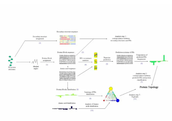
Figure 2. Main principles of this study. The first step consisted to extract from a non redundant databank the dihedral
angles of the protein structures. (1) These last allowed to encode the 3D structures in terms of Protein Blocks. (2) Using different assignment algorithms the 3D structures were encoded also in terms of secondary structures. (3) We first analyzed the agreement between secondary structures and PBs. (4) Then, using the amino acid sequences, we computed amino acid occurrence matrices associated to each PB. (5) We used this information to perform Bayesian prediction and from the prediction in terms of PBs, (6) we computed the predicted frequencies of PBs per protein. (7) We analyzed the correspondence between the predicted frequencies of PBs and the class of the proteins (all α, all β or mixed). (8) In parallel, from the true PBs and the amino acids of the proteins, we computed the frequencies of PBs and amino acids per protein. (9) We learnt these frequencies of PBs per protein using an adapted triangular Self-Organizing Maps, named TopKaPi. Then, we analyzed (10) the amino acid distributions in TopKaPi and (11) the different clusters of PBs.
Figure 2 gives the main steps of the research carried out in this chapter and described here.
Data sets: Different sets of proteins were used in this work. The four first ones have
already been used in a recent work [133]: PAPIA from PDB-REPRDB database [149], PDBselect
databank [150, 151], culled-Pdb (now PSICES) [152], SCOP - ASTRAL [143, 153]. We have preferentially used the PAPIA set which is composed of 717 protein chains and 180,854 residues. The set contained proteins with no more than 30% pairwise sequence identity. The selected chains had X-ray crystallographic resolutions less than 2.0 Å and an R-factor less than 0.2. Each selected structure had RMSD value more than 10 Å with every representative chain. A new updated data set (noted PAPIA03) has been composed from PDB-REPRDB database [149] with the same criteria as PAPIA and is composed of 1,407 protein chains and 293,507 residues. We have verified that the amino acid compositions were not significantly modified between the two protein sets. Each chain was carefully examined with geometric criteria to avoid bias from zones with missing density.
Figure 3. Backbone representation of the 16 Protein Blocks with MOLMOL software [162]. PB a to PB p are
displayed from left to right and from top to bottom.
Protein Blocks (PBs): The structural alphabet we defined in a previous study [128] is
composed of 16 local prototypes called “Protein Blocks” (PBs). They are overlapping fragments of 5 residues in length, encoded as sequence windows of 8 consecutive (ψ, φ) pairs. They were obtained by an unsupervised classifier similar to Kohonen Maps [154, 155] and Hidden Markov Models [156]. Figure 3 gives a representation of the 16 Protein Blocks. The PBs m and d correspond to the prototypes for the central α-helix and the central β-strand, respectively. PBs a through c primarily represents β-strand N-caps and e and f, C-caps. PBs g through j are specific to coils, PBs k and l to α-helix N-caps, and n through p to their C-caps. This structural alphabet allows a reasonable approximation of the protein 3D-structures with a RMSD now evaluated at 0.42 Å. This value has been assessed again in this study with the new databanks.
Protein coding: Protein structures are encoded as sequences of φ - ψ dihedral angles, so that a protein of M amino acids long is defined by a signal of 2(M-1) dihedral angular values.
Each fragment of M residues (M=5) centered at the α-carbon Cαn is represented by a vector of 8
dihedral angles (Ψn-2, Φn-1, Ψn-1, Φn, Ψn, Φn+1, Ψn+1, and Φn+2). The fragment is compared
to each PB with the RMSDa measure [121], i.e. Euclidean distance using angle values. The lowest RMSDa value for the 2(M-1) angles determines the assignment of the PB (Fig2, arrow 1).
Secondary structure assignments: They have been done with ten distinct softwares. The
seven first ones correspond to DSSP [101] (CMBI version 2000), DEFINE [108] (version 2.0), PCURVE [109] (version 3.1), STRIDE [104], PSEA [110] (version 2.0), XTLSSTR [111], SECSTR [24] (Table 2). Default parameters were used for each softwares. Three more programs
have been used: HELANAL [113] to analyze the α-helices, EXTENDED-BETA, which corresponds to an alphabet developed in Kevin Karplus’ laboratory to study more precisely the β-strands [140] and PROMOTIF [55]. DSSP was used to define the α-helices analyzed by HELANAL. Hence, we encoded the 3D protein structures in terms of secondary structures using these different algorithms (Fig. 2, arrow 2), and analyzed the correspondence between the secondary structure and the PB assignments (Fig. 2, arrow 3).
Z-score : Amino acid occurrence matrices were computed for each PB and normalized into
Z-scores as follows : Z-score= (nobs (i,x) - nth (i,x))/ √ nth (i,x), with nobs (i,x) the occurrence
number of observing amino acid i in PB x, and nth (i,x) the occurrence number expected. nth (i,x)
= Nx . fi, where Nx and fi denote the occurrence number of PB x and the frequency of amino acid i
in the entire databank respectively (Fig. 2, arrow 4). Positive Z-scores, more than a user-fixed
threshold ε (respectively negative, less than -ε) correspond to overrepresented amino acids
(respectively underrepresented).
Prediction of PBs by a Bayesian probabilistic approach: The goal is to predict the optimal
PB for each position along a sequence of length L (Fig. 2, arrow 5). To this end, we used a Bayesian probabilistic approach similar to that proposed in a previous work [128]. We focused on
the conditional probability of observing the PBk given an amino acid chain X, (a1, a2,..., ap),
noted P(PBk / X). Bayes' theorem accomplishes the inversion between the sequence X and the
structure PBk. This leads to:
P(X | PBk) = P(a1 | PBk) x P(a2 | PBk) x....x P(ap | PBk)
A window of length p (p =15 here) is slide along the sequence and centered on a position s. To define the optimal Protein Block, PB* for a given amino acid fragment X at a site in a protein,
we used the prediction score Rk:
Rk =P (X | PBk) / P(X) = P(PBk | X) / P(PBk)
The ratio Rk measures the information provided by the knowledge of the amino acid chain X
in the prediction of the Protein Block PBk. This criterion is equivalent to a ratio of likelihood's.
The optimal structural block PBk among the 16 possible blocks is defined as PB* = argmax{Rk}.
Then PB* is assigned to the central residue of the chain X. The final prediction rate, noted Q16, is
the ratio between the number of PBs correctly predicted and all the PBs of the protein.
To assess the prediction, the databank was divided into two sets. The first one was used to
define the PBs sequence-structure relationship and hence to compute : P(PBk / X). The second set
was used to perform the prediction.
To improve the prediction rate, we used the concept of the sequence families which lies on the fact that a local fold can be associated to different clusters of sequences. The initial prediction rate was of 34.2% and was improved to 40.7% [128]. Now, with a new approach (manuscript in
preparation), the prediction rate reaches 48.7%.
Protein classes assignment: To define for a protein its class, we have used the definition of
Michie and co-workers: an all-α protein is characterized by a frequency of α-helix of more than 60% and of β-strand less than 15%, and, an all-β protein by a frequency of α-helix of less than
15% and of β-strand of more than 35% [148].
Analysis of the protein structural classes from the prediction in terms of PBs: the predicted
PBs frequencies per proteins were computed from the results of the Bayesian prediction. They were analyzed using a Principal Component Analysis (PCA) [157] in regards to their structural classes [148] (all α, all β or mixed) (Fig. 2, arrows 6 and 7).
Prediction of the structural classes from the prediction in terms of PBs: For the 3 structural
classes, mean values of each predicted PB frequencies were computed. The prediction step is a comparison between the each target protein predicted PB frequencies and the mean values for the 3 structural classes using an Euclidean distance. The smallest distance defines the assignment to the predicted class.
TopKAPi. In parallel, we computed the true PB frequencies per protein (Fig. 2, arrow 8)
and learnt them using a Self-Organizing Map, named TopKaPi for Triangular Kohonen map for Analyzing Proteins (Fig. 2, arrow 9). Kohonen Map or SOM (Self – Organizing Map) is an efficient way to classify data [155]. The analysis of the results is highly facilitated by the nearness of related clusters. The main specificity of our SOM, is to be a triangle. It is composed
of w = G x (G-1)/2 neurons (triangle side of G neurons). A neuron wt is similar to the vector v
(dimension 16). The learning is iterative and consists in 5 consecutive steps:
(i) random choice of an observation vector v .
(ii) v is compared to every w neurons using an Euclidean distance.
(iii) the winning neuron w* , the closest to v, is identified, i.e. the Euclidean distance is
minimal.
(iv) each neuron wt of the SOM is modified :
w
t+1 <- w
t+ (v - w
t) α(n) π(n)
with α(n) the learning factor and π(n) the neighbourhood factor α(n) is defined as α0 / (1 +
(n / N)), with α0 = 5 /1000, n the number of observation vectors learnt and N the total number of
observation vectors. π(n) controls the diffusion process and is defined by exp(-2(r-r*)2/ ρ(n)2), r
is the coordinates of the neurons wt, r* the coordinates of the winning neuron w*, ρ(n) = ρ0 / (1 +
(n / N)) with ρ0 = 2.4.
(v) the process is reiterated from (i) to (iv) with another vector.
(vi) To learn all the observation vectors of the databanks, the whole databank is used C
times (C = 50).
Then, we analyzed the correspondence between the different clusters obtained and the relationship between local structure in terms of PB distribution and frequencies of amino acids (Fig. 2, arrows 10 and 11).
stride psea pcurve define xtlsstr secstr dssp 95.28 80.40 77.56 61.81 80.36 93.53 stride 81.44 77.99 62.07 80.50 91.40 psea 83.26 64.66 75.90 80.11 define 64.92 60.11 61.55 pcurve 74.56 77.38 xtlsstr 79.47
Table 3. Agreement rate between the different states defined by seven secondary structure assignment methods.
Part I: Secondary structures and PBs
Correspondence between the different secondary structure assignment methods. The
secondary structure definitions are often considered as fixed and the assignment unique [4, 5]. However, as we have noted in the introduction, the reality is less simple. Table 3 gives the agreement ratios between the different Secondary Structure Assignment Methods (SSAMs). These values are computed as the proportion of identical assignment between two SSAMs. To compute these ratios, we have carried out for the SSAMs with more than 3 states a reduction of their N states to a classical 3-state alphabet (helix, extended and coil). We have done the classical
associations for the helicoidal states (i.e. α-helix, 3.10 –helix and π-helix), the extended states (i.e.
extended strand and β-sheet) and the coil state (the other states: turn, bend, polyproline II and coil), even if these associations are not always pertinent. Table 3 shows that two SSAMs can strongly disagree.
A first cluster of SSAMs can be distinguished with DSSP [101], STRIDE [104] and SECSTR [24], which have agreement rates within the range [91.4%; 95.3%]. These 3 SSAMs will be noted DSS (DSSP – STRIDE – SECSTR). They have in common a similar assignment criterion, i.e. the hydrogen bonds computation. Interestingly, between these three methods, the extended structures are not the ones that have the most disruptive assignment. When a divergence in the assignment occurs, in 80% of the case it is between the helicoidal state and the coil state. This fact is particularly clear for SECSTR which was designed to better assign the less frequent
helicoidal states (3.10 and π-helices).
When different assignment criteria are compared (e.g. distances or angles), the agreement rates are within the range [75.9%; 83.2%] for DSS, PSEA [110], PCURVE [109] and XTLSSTR [111]. DEFINE [108] is clearly an outlier SSAM. It creates long successions of identical states,
and its helix frequency is only equal to 27%. This value is largely inferior to all the other SSAMs since the helix frequency is always greater than 31%. Moreover, it is the only one to create high assignment confusion between helix and strand. This awkward confusion is within the range [2% - 5%] between DEFINE and all the other methods. For the others, this confusion α / β is always less than 0.05%. Thus, we show that the definition of new rules and methods since the beginning of the 90’s has not changed the heterogeneity of the secondary structure assignments and that the remarks of Woodcock and co-workers [114] about the difficulties of comparing different assignment methods still remain true.
Example of a protein coding using different secondary structure assignment methods.
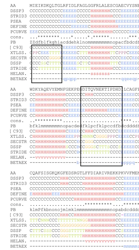
Figure 4 gives the example of the secondary structure assignments obtained for the Hhai Methyltransferase protein (PDB code: 10MH) using the different SSAMs. As Table 3, this figure highlights the difficulties of comparing these methods.
Firstly, the secondary structures of the Hhai Methyltransferase are assigned with a 3-state alphabet by DSSP, STRIDE, PSEA, DEFINE and PCURVE, and the difficulties of finding a consensus (cons.) between all these methods appear clearly since they are very few stars corresponding to a perfect match between the 5 SSAMs. The main disagreements are observed for the α-helices and β-strands edges and length. With the consensus method (noted C93) described by Colloc’h, Etchebest and co-workers [115] which involves the three oldest methods among these five ones, i.e. DSSP, DEFINE and PCURVE, we observe a rate of complete non agreement (i.e. one method assigns a α-helix, the second one a β-strand and the third one a coil) of 1%.
AA MIEIKDKQLTGLRFIDLFAGLGGFRLALESCGAECVYSNE DSSP3 CCCCCCCCCCCCEEEEECCCCCHHHHHHHCCCCEEEEEEC STRID3 CCCCCCCCCCCCEEEEECCCCCHHHHHHHHCCCEEEEEEC PSEA CCCCCCCCCCCEEEEEECCCCCHHHHHHHHHEEEEEEEEE DEFINE CCCCCCCCCCCCCCCEEEEEECHHHHHHHHHHEEEEEEEE PCURVE EEECCCCCCCCEEEEECCCCCCCHHHHHHHCCCCCCEEEC cons. ...********....*...*.******...***. PB ZZdfblfkghiacddehklnommmmmmmmnopacfbdcdf [C93] CCCCCCCCCCCCEEEEECCCCCHHHHHHHHCCCEEEEEEC XTLSS. CPPCEEETTTTEEEEEECTTTHHHHHHHHTTCPPPCEEEC SECSTR CCCCCCCGGGGCEEEEECCCCCHHHHHHHCCCCEECCEEC DSSP CCCCSSCTTTTCEEEEESCTTCHHHHHHHTTTCEEEEEEC STRIDE CCCTTTTTTTTTEEEEETTTTTHHHHHHHHCCCEEEEEEC HELAN. ---sssssss--- BETAEX ---qpqpp---qqeeqp- AA WDKYAQEVYEMNFGEKPEGDITQVNEKTIPDHDILCAGFP DSSP3 CCHHHHHHHHHHHCCCCCCCHHHCCCCCCCCCCEEEEECC STRID3 CCHHHHHHHHHHHCCCCCCCCCCCCCCCCCCCCEEEEECC PSEA EEHHHHHHHHHHCCEEEEECCCCCCCCCCCCCCEEEECCC DEFINE EEHHHHHHHHHHHHEEEEEEHHHHHHHHEEEEEEEEEEEE PCURVE CCHHHHHHHHHHCCEEEECCCCCCCCCCCCCCEEEEEEEE cons. ..**********...****... PB bfklmmmmmmmnopacdedfklpcfklpccdfbdcddddf [C93] CCHHHHHHHHHHHCEEEECCHHHCCCCCCCCCEEEEEEEE XTLSS. CHHHHHHHHHHHHEEEPPCNNNNCGGGGPPPCEEEECCPP SECSTR CCHHHHHHHHHHHCCCCECCGGGCCCCCCCCCCEEEEECC DSSP CCHHHHHHHHHHHSCCCBCCGGGSCTTTSCCCSEEEEECC STRIDE CCHHHHHHHHHHHCCCCBCTTTTTTTTTTCCCCEEEEECC HELAN. --vvvvvvvvvvv--- BETAEX ---b---ppppq-- AA CQAFSISGKQKGFEDSRGTLFFDIARIVREKKPKVVFMEN DSSP3 CCCCCCCCCCCHHHCCCCCCHHHHHHHHHHHCCCEEEEEE STRID3 CCCCCCCCCCCHHHCCCCCHHHHHHHHHHHHCCCEEEEEE PSEA CCCCCCCCCCCCCCCCCCCCHHHHHHHHHHCCCCEEEEEE DEFINE EHHHHHHHEEEHHHHHHHHHHHHHHHHHHHHHHHEEEEEE PCURVE CCCCCCCCCCCCCCCCHHHHHHHHHHHHHHHCCEEEEEEE cons. ...**********....****** PB klmPfkbnonojmlmklmmmmmmmmmmmmnopabdcdddd [C93] CCCCCCCCCCCHHHCCHHHHHHHHHHHHHHHCC-EEEEEE XTLSS. TTTCNNNCCCTTTTTTTNNGGHHHHHHHHHHCCEEEEEEE SECSTR CCCCCCCCCCCGGGGGGGGGGGHHHHHHHHHCCCEEEEEE DSSP CTTTCSSSCCCGGGSTTTTTHHHHHHHHHHHCCSEEEEEE STRIDE TTTTTTTTCCCGGGTTTTTHHHHHHHHHHHHCCCEEEEEE HELAN. ---vvvvvvvvvvv--- BETAEX ---mmmmmz
Figure 4. Example of multiple secondary structure assignments for the N-terminal extremity of the protein 10MH
with DSSP3 and STRID3 (DSSP and STRIDE reduced to 3 states), PSEA, DEFINE, PCURVE, a consensus method (cons. with a star when the 5 methods agree), the consensus defined by Colloc’h and co-workers ([C93]), XTLSSTR, SECSTR, DSSP, STRIDE, HELANAL and the extended BETA alphabet (BETAEX). For the labels see Table 2.
Box 2 Box 1
Secondly, the secondary structure assignments are represented for the methods that give more than three states and the results are even more difficult to analyze. For instance, at the N-terminus of the protein (box 1), when XTLSSTR assigns two positions as PolyProline II followed by a strand and a series of turns, DSSP shows a small bend followed by a turn, STRIDE a longer
series of turns, and SECSTR assigns a 310 helix instead of the turns. The box 2 is another
interesting example, because it reflects classical confusing problems. The 3-state descriptions give a region mainly in coil or with a short helix (except for DEFINE). The consensus C93 also
gives a short helix. SECSTR and DSSP assign a 310 helix which stays coherent with C93.
Nevertheless, XTLSSTR and STRIDE assign those positions as turns. This classical confusion
between 310 helix and turns is the main reason of the exclusion of type III β-turn from the β-turn
classification. In the following positions, we observe the same feature but inversed. XTLSSTR
assigns a 310 helix when STRIDE and DSSP give a turn.
The interest of the Protein Blocks appears through this example. When most of the SSAMs agree, the assigned PBs are coherent with the regular secondary structure states. For instance, the core of the α-helices are described by PB m and the core of the β-strands by PBs c and d. In addition, the PBs give a more detailed description in the confused positions. For example, in box 2, the Polyproline II helix assigned by XTLSSTR has its N-cap characterized by the PBs fklpc, a well characterized series of 5 PBs identified in a previous work as a Structural Word (SW). A SW is a series of PBs which is found with an important occurrence in the databank. The SWs identified have shown a particularly high structural stability [133]. This SW fklpc is characterized by a strong kink which induces a significant change in the backbone orientation. Its last dihedral angles are mainly associated to β-strand values. Thus, it is coherent with a transition between a tight turn and a Polyproline II helix, this last having dihedral angle values in the β-strand upper
left region of the Ramachandran Map.
Figure 5. Example of secondary structure assignments for the protein 10MH with (a) DSSP, (b) STRIDE, (c) PSEA, (d) DEFINE, (e) PCURVE, (f) XTLSSTR and (g) SECSTR. All the methods have been reduced to three states with the helicoidal states in red ribbons, the extended state in green arrows and the coil in blue line.
Figure 5 shows the global 3D structure of the Hhai Methyltransferase according to the seven assignment methods. This picture highlights again the heterogeneity of the secondary structure assignments. For instance, we can note the helices in the upper right of each picture. With DSSP and STRIDE, two helices are found creating an α-α corner, i.e. two helices which are orthogonal [79]. With PSEA, only one helix remains, the shorter one is not considered. DEFINE assigns all in helicoidal state in a surprising way, i.e. even the residues which are in the kink (deviation of 90°). XTLSSTR gives the same result as PSEA, but shorten more the remaining helix. SECSTR, as already noted, does a treatment very similar to DSSP and STRIDE with slight differences at the extremities. With the exception of some particularly well characterized structures like the Schellman box, the precise determination of repetitive structure capping limits is highly difficult [16].
Structu ral alphabet (a ) h elicoidal st ate coil state PB D S . ST . P S . D E . PC. X T . SE . D S . S T . PS. D E . PC. X T . SE . a 0. 13 0.12 0.0 8 15 .9 6 0.0 7 2. 38 0.72 79.80 7 3.55 66.7 7 57 .79 67.5 0 72 .92 82.95 b 0. 29 0.20 0.1 9 11 .3 2 0.0 1 0. 26 1.18 85.55 8 4.73 96.3 2 54 .01 80.2 2 80 .00 98.43 c 0. 02 0.04 0.8 3 15 .2 8 0.0 3 0. 10 0.20 55.42 5 4.26 49.2 0 50 .15 52.5 1 58 .47 57.50 d 0. 00 0.02 0.0 2 9. 13 0.0 1 0. 03 0.00 27.69 2 6.48 19.7 6 40 .30 19.9 9 40 .90 32.29 e 0. 14 0.08 0.0 7 9. 91 0.0 0 0. 04 0.30 47.70 4 6.17 43.7 8 47 .75 55.7 7 65 .51 50.05 f 0. 02 0.05 0.1 1 11 .4 0 0.0 4 18 .49 0.33 71.54 6 9.28 69.9 4 51 .55 78.1 4 64 .95 74.28 g 13 .1 0 11 .9 3 1 0. 63 24 .7 0 1. 69 11. 67 21 .3 5 79.34 7 9.81 84.7 4 58 .81 93.4 4 82 .95 72.95 h 3. 53 2.45 0.3 0 11 .97 0.0 2 0. 22 7.06 76.59 7 6.81 75.7 5 59 .92 88.3 9 89 .32 76.39 i 3. 70 2.36 0.6 0 11 .05 0.0 3 0. 82 10 .3 7 90.20 9 1.01 96.7 9 64 .48 81.6 5 91 .21 89.17 j 10 .63 8.60 0.9 9 12 .68 2.0 2 8.79 12.92 79.05 7 9.65 75.0 0 57 .90 93.5 0 85 .86 80.44 k 47 .69 4 8.91 33.07 22 .96 23.4 7 53 .06 48.21 51.89 5 0.69 66.1 5 56 .86 73.8 6 46 .70 51 .7 4 l 59 .72 5 9.91 41.0 5 29 .34 42.6 0 61 .59 61.14 39.62 3 9.28 58.6 7 55 .20 56.1 0 38 .17 38.46 m 90 .09 9 1.83 85.96 51 .08 86.7 2 91 .70 92.63 9.74 7.98 14.0 1 40 .41 13.2 0 8. 26 7.25 n 67 .99 7 2.36 62.36 44 .0 9 56 .7 8 71. 99 70 .6 4 31.56 2 7.13 37.5 4 46 .41 43.0 0 27 .84 28.88 o 29 .3 0 49 .7 3 3 9. 83 37 .0 7 7. 84 43. 15 28 .9 7 70.20 49 .8 5 59.8 3 52 .19 91.6 8 56 .66 70.72 p 16 .0 5 15 .9 3 9. 48 32 .5 1 1. 90 17. 27 22 .2 7 82.56 8 2.30 86.8 1 54 .93 90.9 7 73 .37 76.55 Ta bl e 4 (a). helico idal and c oil sta te fr eq ue ncies fo r eac h o f the 16 PBs wi th DSSP ( D S.), STRI D E (ST.), PSEA ( P S) , DEFIN E (DE), X T L SSTR (X T) SECS TR(S E).
Structu ral alphabet (b) strand stat e PB DS. ST. PS. DE. PC. XT. SE. a 20 .0 7 26. 32 33 .1 5 26 .2 5 32 .4 3 2 4. 69 16 .3 3 b 14.1 6 15 .07 3.49 34.67 19.76 19.7 3 0. 40 c 44 .5 5 45. 69 49 .9 7 34 .5 7 47 .4 5 4 1. 45 42 .2 9 d 72 .3 1 73. 50 80 .2 2 50 .5 7 80 .0 0 5 9. 08 67 .7 1 e 52 .1 6 53. 76 56 .1 4 42.35 44.23 34.4 6 49 .64 f 28 .4 4 30. 68 29 .9 5 37 .0 4 21 .8 2 1 6. 55 25 .4 0 g 7. 56 8. 25 4. 63 16 .4 9 4. 87 5 .37 5. 71 h 19 .8 8 20. 74 23 .9 5 28 .1 2 11 .5 9 1 0. 46 16 .5 5 i 6.0 9 6. 61 2.61 24.46 18.31 7.9 7 0. 46 j 10.3 3 11 .76 24 .01 29.42 4.48 5.3 6 6. 64 k 0. 43 0. 40 0. 78 20.18 2.67 0. 24 0. 04 l 0. 66 0. 81 0. 28 15.47 1.30 0. 23 0. 41 m 0. 18 0. 20 0. 02 8.51 0.08 0.0 5 0. 13 n 0. 46 0. 51 0. 10 9.50 0.23 0.1 7 0. 48 o 0. 49 0. 42 0. 34 10.73 0.48 0.2 0 0. 31 p 1. 39 1. 75 3. 71 12 .5 6 7. 13 9 .34 1. 17 Ta bl e 4 (b) . ex te nded state fr eq uenci es for each of the 1 6 PBs with DSSP (DS.), STR ID E ( ST .), P S E A ( PS), D E FI N E ( D E), XTLSSTR (XT) an d S E CS TR(S
Moreover, some algorithms are highly sensitive to the quality of the protein structures, i.e. resolution and temperature factors. For instance, a limited change in resolution or temperature factors can modify the DSSP secondary structure assignments.
The Protein Blocks and the classical secondary structure 3-state description. Table 4 (parts
a and b) gives the complete distribution of the 3-state secondary structures for the seven studied methods in the Protein Blocks. As seen in the last paragraphs, DEFINE has a distinct behaviour in regards to the other methods, so we will not take it into account in the following sections.
For all the methods, we observe that the PB m is associated to the α-helix with a mean frequency of 90%. The 10% left correspond to coil. The α-helix is also described by the PBs n (67%) and l (54%). The PB d is associated at 72% to the β-strand and at 28% to the coil. These values underline one more time the β-strand definition problem. The main interest of our structural alphabet is a better description of the coil state by PBs i (90%), b (87%), j (82%), p (82%), h (80%), f (71%), o (66%), k (56%), c (54%) and e (51%).
Tables 4a and 4b enable to further analyze the differences between the secondary structure assignment methods. For seven PBs (i.e. PBs a, b, g, i, j, o and p), we observe some significant differences in their secondary structure assignments. For instance, the PB o has an α-helix frequency of 29.3 % and a coil frequency of 70.2% with DSSP whereas these frequencies are equal to 49.7% and 49.9%, respectively with STRIDE, although these two methods are really close. The PBs g, i and p also present high variations in their α-helix and coil frequencies according to the different methods. The PB a shows high differences with β-strand and coil frequencies of 20.0 % and 79.8% with DSSP versus 26.3% and 73.6% with STRIDE. Furthermore, its β-strand frequency is only equal to 16.3% with SECSTR. A low value of
SECSTR compared to DSSP and STRIDE is also observed for PBs b and i: the β-strand frequencies of PB i and b are equal to 6.1% and 14.1% for DSSP, to 6.6% and 15.1% for STRIDE and only 0.5% and 0.4% for SECSTR. This last point is intriguing as SECSTR was specifically dedicated to perform a better assignment of the helicoidal states than DSSP and STRIDE while giving a similar assignment for the extended state.
We compare all the SSAMs according to their 3-state secondary structure frequencies in the different PBs. For the helicoidal state, we observe a hierarchy XTLSSTR > DSS > PCURVE > PSEA in the frequencies associated to PB m. For the extended state, it is the inverse for the frequencies characterizing the PB d, with XTLSSTR < DSS < PCURVE < PSEA. Finally, for the coil state, we can roughly note the hierarchy PSEA > PCURVE > DSS > XTLSSTR.
The Protein Blocks and the secondary structure N-state description. Table 5 focuses on
three SSAMs that describe the secondary structures with more than three states, i.e. DSSP, STRIDE and SECSTR, and shows the correspondence with the PBs. The helicoidal state is
characterized by α-helices, 3.10 –helices and π-helices. For the α-helix state, the frequencies in
the different PBs are close except as previously noted for the PB o which has an α-helix frequency equal to 22.2% for DSSP, 41.4% for STRIDE and only 14.5% for SECSTR. All the
α-helix frequencies are lower for SECSTR. However, it is the opposite for the 3.10 –helices and in a
lesser extent for the π-helices, since for the PBs from g to p the 3.10 –helix frequencies are 2 to
10% greater than DSSP and STRIDE. This last fact is consistent with the main purpose of
SECSTR. The PB l has a 3.10 –helix frequency of 19.2%. The PB g and p are also especially well
furnished with 3.10 –helix frequencies of about 17%. The π-helix frequencies are low, but far
superior with SECSTR.
Structu ral alphabet (a) α - hel ix 310 - hel ix π - helix PB DSS P S T RIDE SE C S TR DSS P S T RIDE SECS TR DSS P S T RIDE SECS TR a 0.07 0.06 0.0 9 0.05 0. 04 0.6 0 0.01 0.02 0.0 3 b 0.15 0.14 0.1 9 0.12 0. 06 0.9 5 0.02 0.00 0.0 4 c 0.01 0.04 0.0 3 0.01 0. 00 0.1 7 0.00 0.00 0.0 0 d 0.00 0.02 0.0 0 0.00 0. 00 0.0 0 0.00 0.00 0.0 0 e 0.03 0.02 0.0 3 0.09 0. 04 0.2 4 0.02 0.02 0.0 3 f 0.02 0.04 0.0 7 0.00 0. 01 0.2 6 0.00 0.00 0.0 0 g 4.55 4.56 4.0 2 8.52 7.37 17.2 6 0.03 0.00 0.0 7 h 0.43 0.04 0.4 8 3.08 2.39 6.5 6 0.02 0.02 0.0 2 i 0.57 0.02 0.5 5 3.11 2.32 9.8 0 0.02 0.02 0.0 2 j 5.24 4.43 4.7 5 5.34 4.17 8.1 2 0.05 0.00 0.0 5 k 34 .68 35.51 32.3 7 12.99 13 .39 15.7 9 0.02 0.01 0.0 5 l 43 .42 43.47 41.7 6 16.25 16 .40 19.2 0 0.05 0.04 0.1 8 m 85 .64 87.29 81.9 5 4.39 4.49 9.8 3 0.06 0.05 0.8 5 n 60 .40 62.20 57.5 7 7.57 10 .14 12.5 4 0.02 0.02 0.5 3 o 22 .19 41.36 14.4 9 7.10 8.36 14.2 4 0.01 0.01 0.2 4 p 4.56 6.26 4.6 2 11 .49 9.67 17.5 6 0.00 0.00 0.0 9 Table 5 (a). T he t hr ee helic oi dal states fr equencies fo r each of th e 16 PBs d efi ned b y DSSP, STRI D E a nd SECSTR.
Structu ral alphabet (b) turn b end coil iso. β-b ri dg e e xt en ded s tra nd PB D S SP ST RIDE DSS P DSS P STRI D E S E CST R D S SP S T RIDE D S SP ST RIDE SECS TR a 3.28 3 2.53 16.5 8 59.94 41.02 82 .95 3. 01 3.70 17 .06 22.62 16.3 3 b 11 .7 9 42 .1 4 48 .24 25 .5 2 42 .5 9 98 .43 0. 14 0.15 14 .02 14.92 0.4 0 c 0.47 21 .23 13.3 4 41.61 33.03 57 .50 3. 74 3.38 40 .81 42.31 42.2 9 d 0.11 3.60 5.3 6 22.22 22.88 32 .29 1. 79 1.73 70 .52 71.77 67.7 1 e 1.01 3 0.56 7.9 7 38.72 15.61 50 .05 2. 86 3.00 49 .30 50 .7 6 49.6 4 f 0.52 30 .28 7.4 1 63.61 39.00 74 .28 3. 67 3.74 24 .77 26.94 25.4 0 g 15 .4 9 60 .3 6 35.8 1 28.04 19.45 72 .95 3. 52 3.76 4.04 4.49 5.7 1 h 48 .4 7 64 .9 1 13.8 7 14.25 11.90 76 .39 2. 15 1.94 17 .73 18.80 16.5 5 i 61 .7 9 79 .1 7 21.1 3 7.2 8 11. 84 89 .17 0. 25 0.23 5.84 6.38 0.4 6 j 26 .7 8 42 .0 9 31 .47 20 .8 0 37 .5 6 80 .44 1. 83 2.70 8.50 9.06 6.6 4 k 34 .9 1 45 .5 1 10 .27 6. 71 5. 18 51 .74 0. 04 0.01 0.39 0.39 0.0 4 l 24 .36 3 4.90 9.0 2 6.2 4 4. 38 38 .46 0. 25 0.30 0.41 0.51 0.4 1 m 5.36 6.23 1.7 0 2.6 8 1.75 7. 25 0. 10 0.10 0.08 0.10 0.1 3 n 22 .77 2 3.80 4.6 8 4.1 1 3. 33 28 .88 0. 18 0.17 0.28 0.34 0.4 8 o 56 .9 0 41 .00 8.8 1 4.4 9 8. 85 70 .72 0. 39 0.23 0.10 0.19 0.3 1 p 45 .0 0 38 .7 1 17 .46 20 .1 0 43 .5 9 76 .55 0. 25 0.36 1.14 1.39 1.1 7 Ta b le 5 (b ). T urns, b ends, coil , i so late d β-bridg e (iso. β-bridge) an d ex tend ed s tr and stat es f req ue nc ies fo r each of th e 16 PBs defi ned by DSSP, STRI D E SECS TR.
Structu ral alphabet α - heli x exten de d strand PB short lin ear curved ki nk ed una. b p q a z m e a 0. 04 0. 00 0. 00 0. 03 0. 00 3.05 0. 38 1.96 1.6 3 11.4 4 0. 47 0. 92 b 0. 08 0. 00 0. 04 0. 02 0. 00 0.14 0. 02 0.18 0.0 2 0.2 3 0.0 1 13.4 8 c 0. 01 0. 00 0. 00 0. 00 0. 00 3.71 3. 93 7.65 6.1 4 20.75 1.7 9 0.5 3 d 0. 00 0. 00 0. 00 0. 00 0. 00 1.77 8. 03 9.97 17.81 29.39 4.7 7 0.6 7 e 0. 02 0. 00 0. 00 0. 02 0. 00 2.95 6. 05 6.66 8.7 7 25.1 3 2.1 5 0.5 4 f 0. 01 0. 00 0. 00 0. 01 0. 00 3.61 1. 15 4.98 1.5 0 16.24 0. 49 0. 33 g 1.8 5 0 .14 1.03 1.3 0 0.0 0 3.59 0. 00 0.95 0.0 4 2.5 7 0. 11 0. 46 h 0. 18 0. 00 0. 00 0. 25 0. 00 2.15 2. 37 3.41 1.2 7 8.8 6 0.2 9 1.3 8 i 0. 21 0. 00 0. 00 0. 30 0. 00 0.24 0. 00 0.16 0.0 0 0.1 6 0.0 0 5.3 3 j 1.4 8 0. 59 2.42 0.6 9 0.0 5 1.88 0. 00 1.93 0.5 6 4. 16 0. 05 1. 83 k 13.5 2 2 .99 15 .31 2.6 8 0.1 2 0.04 0. 00 0.01 0.0 0 0.0 2 0.0 0 0.3 5 l 16.7 6 3 .75 19 .08 3.5 2 0.1 8 0.23 0. 00 0.07 0.0 1 0.1 7 0.0 1 0.1 5 m 17.5 2 8 .47 48 .63 10.3 4 0.5 8 0.10 0. 00 0.02 0.0 0 0.0 5 0.0 0 0.0 0 n 18.6 1 5 .74 29 .08 6.3 1 0.2 9 0.19 0. 00 0.15 0.0 0 0.1 3 0.0 0 0.0 0 o 6. 92 1. 93 10 .6 3 2. 43 0.1 1 0.36 0. 00 0.00 0.0 1 0.0 3 0.0 1 0.0 3 p 2.0 6 0 .34 1.38 0.7 1 0.0 1 0.26 0. 00 0.01 0.0 2 0.9 4 0.0 0 0.1 8 Ta b le 6. A na ly si s of t he r ep et itive struct ur es de fi ne d by D S SP in ter m s o f Pr ot ei n Bl oc ks. T he α -heli ces are di vi de d in to 5 categories as short helices, l he lices, cur ved h elices, ki nk ed h el ices and u nassign ed h eli ces (una.) using HELANA L . The ex ten ded strands ar e descr ibed a s re si due i n iso la ted β-bridge ( as ex tend ed strand i n : par al le l i n sheet ( p), p ar all el ed ge (q) , anti par al lel sh ee t (a) , an tip ar all el edg e ( z), pa ra llel and a nt iparallel m ixe d ( m ) and str and, al one (e).
The coil state defined in Table 4 is decomposed in four categories, namely the coil (‘C’), the turn (‘T’), the bend (‘N’) and the isolated β-bridge (‘B’). As observed in Table 4, the non-repetitive structures present equivalent frequencies in the different PBs according to the three SSAMs. However, Table 5 shows that between the different types of classification, the results are clearly distinct. The turns of DSSP (states ‘T’ and ‘N’) are not equivalent to the turns of STRIDE (‘T’). Their average frequencies per PBs differ by more than 10%. The turns of DSSP are more frequent in PBs o (+25%), p (+25%), b (+19%) and j (+17%) and the turns of STRIDE (‘T’) are more frequent in PBs f (+21%), e (+21%), a (+11%) and g (+7%). This point is particularly important as the turns are commonly used to describe more precisely the protein structures. For the isolated β-bridge (‘B’), the frequencies are really similar between DSSP and STRIDE, the difference between the two assignment methods is always less than 0.9%. For the extended strand, the results are the same as previously found. These results highlight the complexity of describing only particular regions. The differences in the number of analyzed local folds can bias the analysis of the results.
The Protein Blocks and the precise description of the repetitive secondary structures. Table
6 summarizes the distribution of the α-helices and extended strands using more detailed descriptions.
The helices of the Protein DataBank [102, 103] are known not to be ideal helices according to the thermodynamical properties. The use of the SSAMs often creates helices that are too long. The longest helices in the Protein DataBank contain about 60 residues. Barlow and Thornton [112] have shown that 3/4 of the helices are not linear, i.e. they are curved or kinked. HELANAL [113] allows to redefine helices into 5 categories: short (less than 9 residues), linear, curved,
kinked or unassigned. We have used DSSP definitions of the helices to compute the assignment. As expected, the most frequent PB associated with the different categories is PB m with 48.6% associated to curved helices, 17.5% to short helices, 10.3% to kinked helices and only 8.5% to linear helices. PB m represents 70.1% of the PBs associated to short helices, 82.6% to linear helices, 84.2% to curved helices and 84.4% to kinked helices. We observe that the short helices are described by several other PBs including PB n (18.6%), l (16.8%) and k (13.5%), with PB n frequency greater than that of PB m. For the other types of helix, PB m remains the most important although for the curved helices for instance many other PBs are involved in their description.
In the same way than for HELANAL, the extended beta alphabet used the DSSP outputs to define different new labels : isolated β-bridge (‘b’), extended strand in parallel sheet (‘p’) or parallel edge (‘q’), antiparallel sheet (‘a’), antiparallel edge (‘z’), parallel and antiparallel mixed (‘m’) and strand only (‘e’). As expected, the PBs d, c and also e are the most frequent ones. In addition, two interesting facts must be pointed out. The first one is the isolated β-bridge (‘b’) which is characterized by the PB g with a frequency of 3.6% even though it is not a PB
particularly associated to extended structures. The second one is the distribution of the extended
strand alone (‘e’) which is mainly associated to the PB b, a PB associated with long loops and Ccap of β-strand, and to PB i, which is more associated to the coil state than to the extended state.
These results show that even for the repetitive not-so ideal structures, the Protein Blocks constitute an interesting analyzing tool.
Structu ral alphabet hel ix tu rn s PB α 310 3 10 Ccap h. -b onded un h.-bon d PII PII Ccap coi l ex tended a 1.64 0. 73 0. 01 3.34 2. 07 22 .15 0. 42 44 .94 24 .69 b 0.14 0.0 1 0. 11 9.31 7. 40 0. 91 0. 03 62 .35 19 .73 c 0.06 0.0 2 0. 02 0.66 0. 75 23 .13 5.36 28 .57 41 .45 d 0.02 0.0 1 0. 00 0.24 0. 37 17 .09 4.80 18 .40 59 .08 e 0.04 0.0 0 0. 00 12.14 3. 19 19 .96 5.64 24 .58 34 .46 f 12.77 5.7 2 0. 00 12.19 4. 04 0 .56 24 .96 23 .20 16 .55 g 4.17 0.1 1 7. 39 23.54 7. 81 14 .70 0.35 36 .55 5. 37 h 0.20 0.0 2 0. 00 35.09 6. 92 1 .69 23 .51 22 .11 10 .46 i 0.73 0.0 9 0. 00 39.17 5. 87 2 .10 0. 16 43 .91 7.97 j 6.13 2.6 6 0. 00 34.63 8. 02 0. 05 0. 31 42 .85 5.36 k 36.93 16.1 3 0. 00 31.42 9. 09 0. 02 0. 07 6. 10 0. 24 l 43.18 18.4 0 0. 01 24.89 7. 68 0. 13 0. 13 5. 34 0. 23 m 75. 73 13.1 1 2.86 4. 49 1.60 0. 02 0. 01 2. 14 0. 05 n 52.45 14.4 4 5.10 14.10 4. 24 0. 10 0. 21 9. 19 0. 17 o 30.05 1.8 8 11 .22 28.11 5. 21 0. 09 0. 03 23 .22 0. 20 p 4.48 0.3 3 12 .46 11.39 2. 67 0. 21 0. 00 59 .10 9. 34 Ta b le 7. Cor respon dence bet w een th e states def in ed by XTLS STR and th e 16 Protei n Bl oc ks wi th th e α -h el ix , t he 3 10 h eli x and its Ccap, the tu rns de fi ne d by t pr esence (h .-bo nded ) or ab se nce ( unh.-bo nd ) of an hydroge n s tabil iz ing b ond, t he poly pr ol ine II ( PI I) a nd it s Ccap, coil an d ex te nded stran d.
The Protein Blocks and XTLSSTR 9-state description. Table 7 summarizes the
correspondence between the 16 Protein Blocks and the 9 states defined by XTLSSTR. This method has some interesting particularities like the assignment of turns not with the classical dihedral angle criteria but defined as hydrogen- or non hydrogen bonding-turns, and of
polyproline II helices. Moreover, it identifies the Ccaps of the 3.10 –helices and of the polyproline
II helices. This SSAM gives different results in regards to the precedent methods. The PB f is
now associated with a non negligible proportion of α-helix (12.7%) and of 3.10 –helix (5.7%).
This last fact is related to the PB g 3.10 –Ccap frequency (7.4%) since the main transition of PB f
is PB g. This value is coherent with the DSS frequency of 3.10 –helix associated to PB g (DSSP,
STRIDE and SECSTR frequencies are equal to 8.5%, 7.4% and 17.3%, respectively; cf. Table
5a). The PBs o and p are associated to the 3.10 –Ccap (frequencies of 11.2% and 12.5%,
respectively). In addition, we observe that globally more hydrogen bond turns are found than unhydrogen bond turns. Several PBs are involved in their description with no particular specificity related to the hydrogen bond stabilization. As for the polyproline II helices, they appear more frequent in globular proteins than expected [23]. Their dihedral angle distribution is often confused with β-strands in the upper left of Ramachandran Map and so is confused with the β-sheet assignment. This feature is observed again in these results where PBs a, c, d, e and g have polyproline II frequencies equal to 22.1%, 23.1%, 17.1%, 20.0% and 14.7%, respectively. Some PBs are specific to the C-cap of the polyproline II helix, e.g. PBs f and h. These observations are in agreement with the main transitions between successive PBs since PB e often goes to PB f and PB g to PB h.
Thus, the goal of this detailed analysis was to emphasize the fact that the “classic”
secondary structures can be described with different criteria which results in ambiguous assignments. Moreover, we have highlighted the interest of using more than three states for better describing protein structures through a structural alphabet. The 16 PBs enable to analyze specifically every part of the protein structures.
In the next section of this chapter, we propose a prediction scheme of the protein structural classes from the PB prediction.
Part II: PBs and protein structural classes
Goal. The question tackled in this section is the potentiality of classifying one protein into
its true protein class from the sole knowledge of its prediction in terms of Protein Blocks. The process used is in three steps : (i) Protein Blocks are predicted from the sequence, (ii) the relative frequencies of the 16 PBs are computed and the three mean frequencies vectors, called prototypes, representing the three protein classes are computed from the learning protein set (iii) the comparisons between the three mean prototypes representing the protein classes and the relative frequencies of the 16 PBs are done for target proteins to predict their classes.
Having a good idea of the protein classes can be an efficient way for refining the prediction research. For instance, it can enable to direct the prediction of a protein, i.e. if a protein is all-α, the information derived from all-β proteins would not be used for this protein. The interest of this study is not to use the true PBs, but the predicted PBs. The prediction rate is, as previously said, equal to 40.7% [128]. Hence, the difficulty here is to predict accurately protein classes from this partial information.
Protein classes. As noted by Thornton and co-workers, the secondary structures form
particular motifs that define the global protein topology, e.g. the TIM barrel fold [141]. This information is used to classify the protein structures. Different algorithms have been developed and the classification is done either automatically like in the CATH database [144] or mainly manually like in the SCOP database [143]. Different classes are defined and give information about the relationships between the proteins. Interestingly, the different methods give the same types of hierarchical relationships with few superfamilies and many subfamilies. On the basis of their secondary structures, the folds are grouped into four main classes: all-α (essentially α-helices), all-β (essentially β-strands), α + β (α−helices and β-strands are largely segregated) and α / β (α−helices and β-strands are largely interspersed). The assignment of a structure to a particular class is in some cases a difficult task. In fact, even with an automatic classification, a manual inspection is needed. From the sole knowledge of the amino acid sequence, the task is even more complicated when no homologous sequence is found.
Bayesian prediction of the Protein Blocks: In a previous study [128], we have tackled the
Protein Blocks prediction from the amino acid sequence. To this end, we extracted the amino acid preferences for each local pattern and used this information in a Bayesian process to predict the structural motifs able to be adopted by a given protein chain. With this strategy, for each amino acid sequence, the potential series of Protein Blocks is predicted [128, 133]. To evaluate the
prediction, we computed a Q16 ratio which corresponds to the number of well predicted PBs. This
value is similar to the Q3 of secondary structures with more states to predict, i.e. N=16
possibilities against N=3 for the secondary structures.
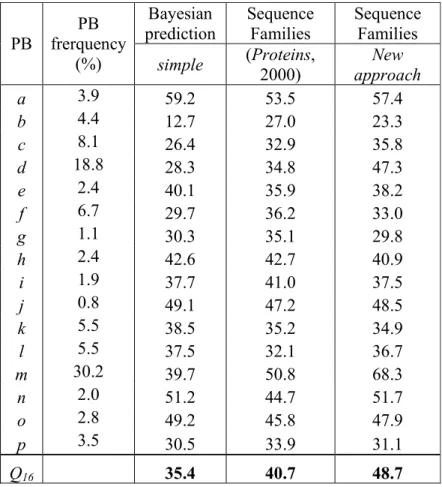
Table 8. Bayesian prediction with Q16 value for the 16 Protein Blocks with their corresponding frequencies and
prediction rate for the (simple) Bayesian prediction and the improved prediction using the sequence families with the original results (Proteins, 2000) [ADB00] and the new one (new approach).
With the new databank used in this study, we have an initial Q16 ratio equal to 35.4%, which
is very similar to the result of our previous work, i.e. 34.4% [128]. Table 8 (col 3) gives the prediction rates for each of the 16 PBs. The high differences of the PB frequencies in the databank need to be taken into account (Table 8, col 2) since some of the PBs are overrepresented
like PBs m and d (30.2% and 18.8% respectively). Consequently, we made sure that the Q16 ratio
was not biased by over-predictions of PBs m and d.
However, associating one PB with one class of sequences is a restrictive point of view. A Bayesian prediction Sequence Families Sequence Families PB PB frerquency
(%) simple (Proteins, 2000) approach New
a 3.9 59.2 53.5 57.4 b 4.4 12.7 27.0 23.3 c 8.1 26.4 32.9 35.8 d 18.8 28.3 34.8 47.3 e 2.4 40.1 35.9 38.2 f 6.7 29.7 36.2 33.0 g 1.1 30.3 35.1 29.8 h 2.4 42.6 42.7 40.9 i 1.9 37.7 41.0 37.5 j 0.8 49.1 47.2 48.5 k 5.5 38.5 35.2 34.9 l 5.5 37.5 32.1 36.7 m 30.2 39.7 50.8 68.3 n 2.0 51.2 44.7 51.7 o 2.8 49.2 45.8 47.9 p 3.5 30.5 33.9 31.1 Q16 35.4 40.7 48.7

![Figure 3. Backbone representation of the 16 Protein Blocks with MOLMOL software [162]](https://thumb-eu.123doks.com/thumbv2/123doknet/14215109.482647/17.892.189.721.593.1032/figure-backbone-representation-protein-blocks-molmol-software.webp)