Characteristics of North Sea Oil Reserve Appreciation
by
00-008 December 2000
G.C. Watkins
1/29/01 11:00 AM
CHARACTERISTICS OF NORTH SEA OIL RESERVE APPRECIATION
G.C. Watkins
Massachusetts Institute of Technology, Cambridge, USA and University of Aberdeen, Scotland, UK
CHARACTERISTICS OF NORTH SEA OIL RESERVE APPRECIATION* G.C. Watkins
Massachusetts Institute of Technology, Cambridge, USA and University of Aberdeen, Scotland, UK
December 2000
Abstract. In many petroleum basins, and especially in more mature areas, most reserve additions consist of the growth over time of prior discoveries, a phenomenon termed reserve appreciation. This paper concerns crude oil reserve appreciation in both the UK and Norwegian sectors of the North Sea. It examines the change in reserves attributed to North Sea fields over time, seeking to reveal patterns of reserve appreciation both for individual fields and for groups of fields classified by potentially relevant common elements. These include field size, year of production start-up, geological age, gravity, depth and depletion rate. The paper emphasises the statistical analysis of reserve appreciation. It contrasts the Norwegian and UK experience. An important distinction is drawn between appreciation of oil-in-place and changes in recovery factors. North Sea oil reserve appreciation between production start-up and the last observation year (usually 1996) is found to be substantial, but it generally lacks a consistent profile. Appreciation recorded for the Norwegian fields on average is considerably greater than for the UK. Most UK appreciation is seemingly accounted for by oil-in-place; in Norway, from increases in recovery factors. However, UK recovery factors commence at much higher levels than those for Norway.
*
I wish to thank Samantha Ward of the University of Aberdeen for her extensive, sterling research assistance. I wish to also thank Eric Mathiesen of the Norwegian Petroleum Directorate and Mervyn Grist of the UK Department of Trade and Industry for providing information and advice. Valuable comments were received from Morris Adelman (MIT), Denny Ellerman (MIT), Graeme Simpson (University of Aberdeen), Alexander Kemp (University of Aberdeen), James Smith (Southern Methodist University), Andre Plourde (University of Alberta), Emil Attanasi (US Geological Service), John Schuenemeyer (University of Delaware), and George Warne (World Petroleum Congress). I also thank participants in seminars and workshops at the University of Aberdeen and MIT for advice. The usual disclaimer applies.
TABLE OF CONTENTS
Introduction ... 6
1. RESERVES: BACKGROUND... 7
Reserve Components. ... 7
Oil and Natural Gas Reserve Appreciation ... 8
Technological Change ... 8
Field Development Patterns ... 9
Data Sources ... 11
2. NORTH SEA RECOVERABLE RESERVES: STATISTICAL FEATURES ... 11
Initial Recoverable Reserves ... 11
Distribution of Field Size ... 12
Gross Reserve Appreciation... 13
Distribution of Reserve Appreciation. ... 14
Distribution by Production Life ... 14
Distribution by Water Depth... 14
Distribution by Gravity... 15
Distribution by Geological Age... 15
Distribution by Depletion Rate ... 15
3. RESERVE APPRECIATION PATTERNS AND PROFILES ... 16
Factor Definition ... 16
Appreciation Profiles ... 17
Reserve Appreciation by Individual Field ... 17
Reserve Appreciation by Vintage ... 18
Reserve Appreciation by Water Depth ... 18
Reserve Appreciation by Gravity... 19
Reserve Appreciation by Geological Age ... 19
Reserve Appreciation by Field Size ... 20
Reserve Appreciation by Depletion Rate ... 21
Summary Features ... 21
4. RESERVE APPRECIATION FUNCTIONS ... 23
Similar Analysis... 24
Field Analysis... 24
Field Parabolic Functions ... 24
Field Constrained Functions ... 25
Summary Comment ... 25
5. ANALYSIS OF OIL-IN-PLACE AND RECOVERY FACTORS ... 25
UK ... 25
Norway ... 26
UK Oil-in-Place Appreciation and Recovery Factors... 28
Norwegian Oil-in-Place Appreciation and Recovery Factors……... 28
Validity of Comparisons ... 29
6. CONCLUSIONS ... 31
References ... 32 APPENDIX A: Reserve Statistics... A-1 APPENDIX B: Reserve Appreciation... B-1 APPENDIX C: Appreciation Factor Profiles ... C-1 APPENDIX D: Basic Field Data and Data Sources ... D-1
LIST OF TABLES, FIGURES, AND CHARTS (Main Text)
Table 2-1. North Sea Initial Recoverable Oil Reserves: Summary Statistics... 13
Table 2-2. Size Concentration of Initial Recoverable Reserves at Start-up... 13
Table 2-3. North Sea Gross Reserve Appreciation: Summary Statistics ... 14
Table 2-4. Size Concentration of Reserves Appreciation ... 15
Table 3-1. Reserve Appreciation Factors by Vintage ... ... 20
Table 3-2. Appreciation Factor Summary: UK Sector ... 22
Table 3-3. Appreciation Factor Summary: Norwegian Sector... 23
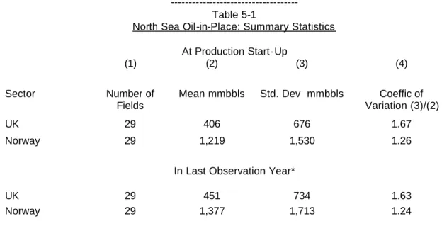
Table 5-1. North Sea Oil-in-Place: Summary Statistics... 27
Table 5-2. North Sea Oil-in-Place Appreciation: Summary Statistics ... 28
Table 5-3. Summary: UK Sector, Oil-in-Place and Recovery Factors ... 29
Table 5-4. Summary: Norway, Oil-in-Place and Recovery Factors ... 30 (Appendices)
Figure A-1. Initial Reserves in Start-up Year: Combined Sectors ... A-1 Figure A-2. Initial Reserves in Start-up Year: UK Sector ... A-2 Figure A-3. Initial Reserves in Start-up Year: Norwegian Sector... A-3 Figure A-4. Initial Reserves in Last Observation Year: Combined Sectors ... A-4 Figure A-5. Initial Reserves in Last Observation Year: UK Sector ... A-5 Figure A-6. Initial Reserves in Last Observation Year: Norwegian Sector ... A-6 Figure A-7. Gross Reserve Appreciation: Combined Sectors ... A-7 Figure A-8. Gross Reserve Appreciation: UK Sector ... A-8 Figure A-9. Gross Reserve Appreciation: Norwegian Sector ... A-9 Figure A-10. Age Characteristics: UK Sector ... A-10 Figure A-11. Age Characteristics: Norwegian Sector ... A-10 Figure A-12. Water Depth Characteristics: UK Sector ... A-11 Figure A-13. Depth Characteristics: Norwegian Sector ... A-12 Figure A-14. Gravity Characteristics: UK Sector... A-13 Figure A-15. Gravity Characteristics: Norwegian Sector ... A-13 Figure A-16. RP Ratio: UK Sector... A-14 Figure A-17. RP Ratio: Norwegian Sector ... A-15 Figure A-18. Oil-in-Place at Start-up Year: UK Sector ... A-16 Figure A-19. Oil-in-Place at Start-up Year: Norwegian Sector ... A-17 Figure A-20. Oil-in-Place in Last Observation Year: UK Sector ... A-18 Figure A-21. Oil-in-Place in Last Observation Year: Norwegian Sector ... A-19 Figure A-22. Oil-in-Place, Appreciation, UK Sector……… ... A-20 Figure A-23. Oil-in-Place, Appreciation, Norwegian Sector ... A-21 Figure A-24. Geological Age: UK Sector ... A-22 Figure A-25. Geological Age: Norwegian Sector ... A-22 Figure A-26. Size Characteristics: UK Sector... A-23 Figure A-27. Size Characteristics: Norwegian Sector ... A-23 Figure A-28. Water Depth Characteristics: UK Sector ... A-24 Figure A-29. Water Depth Characteristics: Norwegian Sector ... A-24 Figure A-30. Gravity Characteristics: UK Sector... A-25 Figure A-31. Gravity Characteristics: Norwegian Sector ... A-25 Figure A-32. RP Ratio: UK Sector……… ...…A-26 Figure A-33. RP Ratio: Norwegian Sector………. ... A-26 Figure A-34. Geological Age: UK Sector……… ... A-27 Figure A-35. Geological Age: Norwegian Sector……… ... A-27
Figure A-36. Size Characteristics: UK Sector………. ... A-28 Figure A-37. Size Characteristics: Norwegian Sector………... A-28 Table B-1. Initial Reserves: Appreciation Factors by Vintage: UK Sector ... B-1 Table B-2. Initial Reserves: Appreciation Factors by Vintage: Norwegian Sector ... B-3 Figure B-1. Reserve Appreciation by Vintage: UK Sector………. ... B-5 Figure B-2. Reserve Appreciation by Vintage: Norwegian Sector………. ... B-5 Table B-3. Oil-in-Place Appreciation Factors by Vintage: UK Sector... B-6 Table B-4. Oil-in-Place Appreciation Factors by Vintage: Norwegian Sector ... B-7 Chart C-1. Appreciation Profiles of Initial Recoverable Reserves: UK Sector ... C-1 Chart C-2. Appreciation Profiles of Initial Recoverable Reserves: Norwegian Sector .. C-10 Chart C-3. Reserve Appreciation Profiles by Vintage: UK Sector……… ... C-13 Chart C-4. Reserve Appreciation Profiles by Vintage: Norwegian Sector…………... C-16 Chart C-5. Appreciation Profiles by Depth: UK Sector………… ... C-18 Chart C-6. Appreciation Profiles by Depth: Norwegian Sector.. ... C-18 Chart C-7. Appreciation Profiles by Gravity: UK Sector………… ... C-19 Chart C-8. Appreciation Profiles by Gravity: Norwegian Sector… ... C-19 Chart C-9. Appreciation Profiles by Geological Age: UK Sector………. ... C-20 Chart C-10. Appreciation Profiles by Geological Age: Norwegian Sector…. ... C-20 Chart C-11. Appreciation Profiles by Size of Field: UK Sector……….. ... C-21 Chart C-12. Appreciation Profiles by Size of Field: Norwegian Sector……. ... C-21 Chart C-13. Appreciation Profiles by RP Ratio: UK Sector………... C-22 Chart C-14. Appreciation Profiles by RP Ratio: Norwegian Sector………… ... C-22 Table C-1. Reserve Appreciation Profiles by Field: Parabolic Curve Fits ...….C-23 Table D-1. Various Field Characteristics: UK Sector ... D-1 Table D-2. Various Field Characteristics: Norwegian Sector ... D-5 Data Sources ... D-7
Introduction
In many petroleum basins, and especially in mature areas, most reserve additions consist of growth in already discovered fields. This phenomenon is termed reserve appreciation. For example, in the US from 1978 to 1991 reserve appreciation accounted for more than 90 per cent of additions to proved reserves1. Hence, the nature and characteristics of reserve appreciation are crucial to understanding petroleum supply. Discovery size estimates require adjustment to reflect future field growth, otherwise the relative efficiency of recent exploration will be undervalued. Moreover, as M.A.Adelman has shown, relationships between field development cost and reserve additions can serve as a proxy for finding cost2.
This paper concerns crude oil reserve appreciation in both the UK and Norwegian sectors of the North Sea, a province that accounts for about two per cent of current world proven remaining oil reserves, eight per cent of production, and acts as a pricing fulcrum. Changes in field reserves are examined to see whether regular patterns of reserve appreciation are revealed for individual fields and for groups of fields classified by common elements3. These include field size, year of production start-up, geological age, gravity, water depth and depletion rate.
Field reserve growth in offshore areas such as the North Sea has not been investigated extensively. Some analysts have been sceptical about potential field growth in such regions, arguing that in high cost areas operators delineate fields more precisely prior to development4. Moreover, investment in pressure maintenance is more likely before production comes on stream, improving well productivity and economic viability. The associated higher recovery factor constrains the scope for reserve appreciation.
Primary emphasis in this paper is placed on the statistical analysis of reserve appreciation. A distinction is drawn between appreciation of oil-in-place - the oil contained in a field, whether recoverable or not - and the proportion estimated as recoverable (the recovery factor). This distinction turns out to be important. The paper does not attempt to discern the influence economic factors might have on appreciation patterns5. Such factors could include prices, tax regimes, technological change, market structure, and different approaches among company operators.
I find that oil reserve appreciation in the North Sea is substantial, contradicting the view that appreciation of offshore fields may be negligible. As a fraction of reserves booked in the start-up year, however, it is not as marked as that in mature onshore areas. This in part does reflect earlier reserve recognition at production start -up, with prompt inception of pressure maintenance. Although appreciation among North Sea fields lacks any consistent profile, noticeable differences among groupings of reserves are disclosed.
The most important distinction to emerge is that between the UK and Norwegian sectors. Appreciation recorded for Norwegian fields is considerably greater than for the UK. In the UK, most appreciation appears to be accounted for by growth in oil-in-place; in Norway, from growth in recovery factors. However, recovery factors in the UK commence at much higher levels than
1
Attanasi and Root [1994, p321].
2
For example, see Adelman [1993].
3
A field is a single reservoir or multiple reservoirs related to the same individual geologic structural feature and (or) stratigraphic condition. Two or more reservoirs (pools) assigned to the same field may be separated vertically by impervious strata or laterally by geologic barriers. Note that field growth can result from finding new reservoirs within a field - often well after the initial discovery, especially onshore. To give one example, in Alberta the Clive D-2B pool was discovered about 20 years after the D2-A pool.
4
Mentioned in Attanassi [2000, p63].
5
those for Norway. Increases in Norwegian recovery factors are akin to catch-up to those recorded by the average UK field.
The paper is organised in six sections. Section 1 deals with background aspects: the definition of oil-in-place and recoverable reserves; the role of technology; the nature of development patterns; and data sources. Section 2 brings together key statistical features of the distribution of North Sea recoverable oil reserves. Section 3 examines patterns of reserve appreciation among fields and field groupings for the UK and Norwegian sectors. Section 4 looks at time profiles of reserve appreciation. Section 5 concerns the appreciation of oil-in-place and implied shifts in recovery factors. This section relies on confidential field data and the results presented are confined to certain aggregates. The conclusions of the paper are presented in Section 6.
Additional, considerable detail is provided in four appendices. Appendix A consists of information on various statistical measures. Appendix B provides background tables on reserve appreciation. Appendix C compiles charts of appreciation factors over time. Appendix D provides summary tables of basic data by field, and information on data sources.
1. RESERVES: BACKGROUND
The discussion below covers the distinction between oil-in-place, initial recoverable reserves and remaining reserves, differences between crude oil and natural gas reserve appreciation, and the role of technological change. It also provides a specific example of how North Sea field development has given rise to reserve re-evaluation.
An initial recoverable oil reserve is an estimate of how much oil at the surface a deposit would eventually yield. Oil-in-place is the estimate of how much oil the deposit originally contained. These estimates are not fixed. They are subject to continual reappraisal. It is the
change in such estimates over time on which this paper focuses. Remaining recoverable
reserves are initial recoverable reserves less cumulative production to date.
Reserve Components. Initial recoverable oil reserves are the product of two components: oil-in-place, and the recovery factor. Oil-in-place is the estimated amount of petroleum in a field, whether the oil can be brought to the surface or not. The recovery factor is the estimated fraction of the oil-in-place that could be brought to the surface over a field’s effective life.
Oil-in-place can be thought of as the volume of oil bearing sediments less all the space not occupied by oil. The ability of oil to flow to the surface is affected by the inherent nature of the reservoir - its permeability and porosity, the amount of water as well as oil clinging to the rock, oil viscosity, various other physical factors, and above all by the physical reservoir drive mechanism propelling oil to the surface once the deposit is tapped.
To be more explicit, for a given field oil-in-place can be written as:
STOIP = c x H x A x POR x (1 - SW) x SHR (1-1) where STOIP = oil -in-place measured at the surface (stock tank barrels)
c = a constant converting acre-feet to barrels (or tonnes) H= pay thickness
A = acreage POR = porosity of the rock
SW= water saturation (1 - SW = oil saturation) SHR = shrinkage factor in bringing oil to the surface.
Equation (1-1) is expressed as if oil were recovered at the surface; the shrinkage factor accounts for the difference between measurement underground at reservoir temperature and
pressure, and that at the surface. Shrinkage mainly arises because underground oil is swollen by dissolved gas. At atmospheric pressure these liquids become gas, reducing the volume of liquids.
Initial recoverable reserves are:
INRES = RF x STOIP (1-2) where INRES = initial recoverable oil reserves (stock tank barrels)
RF = recovery factor.
A distinction can be drawn between primary, secondary and tertiary recovery. The primary recovery factor is that expected to prevail without any action by the field operator - in other words if the field were depleted naturally. Secondary and tertiary recovery factors are those anticipated were the natural drive mechanism augmented by production practices and investment intended for that purpose. Typically these are schemes to maintain reservoir pressure by water injection. Measures to increase eventual recovery are termed enhanced recovery (ER) schemes.
Oil-in-place is governed by a field’s natural physical configuration, as is evident from equation (1-1). It follows that field delineation and information gathered over time on field properties mainly determine revisions to estimates of oil-in-place. Estimates of the recovery factor can also be affected by field delineation. But they are more fundamentally affected by the kind of reservoir development plan pursued and by implementing advances in field technology, allied to accumulation of knowledge about production performance. The crux of the matter is that the dynamics of appreciation of ‘in-place’ reserves may well differ from those governing changes in recovery factors.
Hence, if the data permit it is preferable to breakdown appreciation of recoverable reserves between oil-in-place and recovery factor components. The two elements are not independent. Both are affected by knowledge garnered as reservoir development and depletion proceed.
Oil and Natural Gas Reserve Appreciation. This paper concerns oil. The scope for oil reserves appreciation usually exceeds that for natural gas. This mainly represents inherent differences in primary recovery factors, which for oil are typically around 30 per cent, for gas around 80 per cent. Most increases in gas reserves reflect increases in gas-in-place from extensions in field contours and reassessment of field properties. Increases in oil reserves reflect both increases in oil-in-plac e and in the recovery factor. It follows there is more latitude for changing technology to affect oil reserve appreciation (examined in this paper) compared with that for natural gas. Such differences in reserve appreciation patterns are one of the reasons for excluding natural gas reserves contained within the oil fields comprising the this study's data base.
Technological Change. Over the past decade or so changes in technology have been especially noticeable. The ‘big three’ have been 3D seismology, horizontal and directional drilling, and deep water production systems6. One stimulus behind such innovations has been relatively weak or stagnant oil prices since the mid-1980s until recently, in conjunction with a more competitive industry structure that has placed a high premium on cost efficiency.7
New technologies have inter alia improved drilling success rates, increased reservoir recoveries, and extended exploration prospects. In short, petroleum productivity has risen. The incidence, timing and nature of technological development influence the scope for reserve appreciation.
6
Bohi [1999, p74]
7
‘New technology’ is a broad term, embracing not only hardware embodying new techniques, but also new information systems and modelling techniques. Recent North Sea examples are mentioned below8.
The ‘Seisbit’ system measures the noise of a working drill-bit as a down-hole method of compiling seismic information. Its benefits include minimisation of rig downtime, lower operational risks for both exploration and appraisal wells, and increased accuracy in assessing rock properties in the neighbourhood of the well.
Multi-lateral wells replace two single wells by a dual well without compromising production rates or reserves, and also reduce pressure on available drilling slots. Application to the Forties field in the North Sea entailed development of an adjunct technology called ‘through tubing drilling’ enabling drilling via production tubing. This allows small remaining targets in mature fields to be targeted. The system is reported as being applied successfully to eight platforms and three sub-sea wells in the North Sea and offshore Brazil (Smith Rae [1999, p42])
Optimal reservoir management requires up to date information on the distribution of field fluids. Time dependent measurements improve the accuracy of reservoir models. 3D seismic measurements provide inter-well data. Four dimensional (4D) seismic images (3D plus time) can map fluid changes in a field, hence improving predictions of field parameters offered by simulations. The technique can lead to identification of bypassed oil and undrained reservoir niches. It has been applied by Statoil to the Gullfaks field to improve drainage by drilling a horizontal well, increasing recoverable reserves (Smith Rae [1999, p149]).
The ability of new and modified technologies to be brought to maturity has been enhanced by techniques that improve well drilling, completion, operation and evaluation. Two dimensions are involved: improvements in reservoir modelling; and introduction of new well equipment. The ‘Simpler’ process is an organisational approach to drilling operations resulting in significant cost reductions.
Floating production, storage and offloading (FPSO) units can be deployed on marginal fields, both at remote locations and in deep water. New developments have improved the quantity and quality of data obtained from these facilities, especially in terms of information on vessel fatigue. Lifetime prediction model techniques called ‘FPSO Integrity’ are expected to reduce fuel consumption by vessels, to increase positioning accuracy - especially in harsh weather - and to reduce downtime.
Improvements in seismic technology may well have a greater impact on assessments of oil-in-place than on recovery factors. Changes in drilling technology might have a greater relative impact on the recovery factor. Thus the nature and incidence of technological developments could have a differential impact on appreciation by reserve component.
Field Development Patterns. Mention has been made of how field delineation and production history can lead to continual reserve re-evaluation, in addition to that from introducing new technology. A good illustration of this is provided by the history of one now depleted field in the UK sector.9
Production started a decade after discovery. Abandonment was expected some 25 years later. Appraisal drilling commenced late 1973, with the first well drilled to 11,500 feet. One geologic interval tested 10,800 b/d, another 750 b/d. A well drilled to the north of the discovery well found only thin net oil pay. A final appraisal well drilled in 1978 flowed 5,300 b/d.
8
These are drawn mainly from Smith Rae Energy Associates [1999].
9
Development drilling started in 1979 and continued until early 1983. A production platform was installed to handle output from 12 wells. The natural water drive was boosted by six water injection wells - an example of immediate inception of ER. One development well discovered another reservoir. Peak production was reached in 1984. Subsequently, production wells that watered out were converted to injectors or side tracked to deeper targets.
Understanding of the field paralleled growth in the geophysical, geological and reservoir database. The first (two dimensional) seismic data was obtained in 1970. Further 2D data were acquired, but did not induce significant changes in the structural maps. More seismic data were obtained in 1978, confirming the prevailing geological model.
The first reservoir simulation model was constructed in 1974, and updated in 1976. Predicted oil recovery after 10 years was 46 per cent of stock-tank oil-in-place (STOIP). Further sensitivity studies on water injection were made in 1977; at that time, geological reinterpretation reduced the estimated STOIP.
In 1978 the estimated recovery factor was some 52 per cent, based on 14 producers and 7 injectors. In early 1982 a large amount of new data became available, including 2D seismic. These data led to revisions in the field structural map and new correlations. The estimated STOIP rose. Moreover, the new data necessitated revisions to the reservoir model, indicating new locations for injection wells. The 1982 model suggested higher initial recoverable reserves, with a recovery factor now of some 50 per cent.
By early 1985, data were available from 19 development wells, 18 months of production information, and from the reprocessing of an earlier 2D seismic survey. The new information indicated increases in STOIP and recoverable reserves. The geological model was revised. The STOIP rose further; the recovery factor was then estimated at 47 per cent.
The reservoir simulation model was updated in 1987, after well tests had shown the 1985 model underpredicted production. The revised model indicated a recovery factor of 52.5 per cent. New 2D seismic data were obtained in 1988. One observation well was side tracked and discovered another reservoir within the field.
By the mid 1990s significant advances were made in field information, particularly in geophysical acquisition and processing, and in high resolution biostratigraphy. The field was approaching the stage at which its economic life was very sensitive to the oil price. To ensure all economic oil was produced before abandonment, new studies were undertaken. In 1994 a 3D survey was acquired over the whole block. A revised geological model was developed using all core and log data.
A new biostratographic study was commissioned in 1995. And a field wide seismic inversion project was performed. Additional data obtained by these methods on net hydrocarbon pore volume increased the STOIP. Application of the reservoir model increased the STOIP further, and the recovery factor was estimated at 55 per cent.
The results of the geoscience studies in 1995 and 1996 indicated possible targets for infill drilling. Some new producing wells were drilled. The fluid lifting mechanism changed after 1994. Electrical submersible pumps were installed in 5 producing wells. This generated incremental reserves and reduced gas lift dependency, allowing additional gas lift allocation to remaining wells.
Some wells were converted from sea water to produced water injectors in the 1990s. By Dec., 1998 80 per cent of water injection was produced water, reducing disposal of contaminants. A horizontal well drilled in Nov.1996 confirmed the area reached had been swept. New data supported the accuracy of the revised reservoir simulation model.
This history of a field in the UK sector illustrates how reserve appreciation has taken place over a considerable period of time as a function of:
• reservoir development and performance providing new information;
• recalibration of field engineering and geological models in light of new knowledge; • investment in, and application of, new technology.
The inception of enhanced recovery techniques at production start-up is noteworthy. The estimated recovery factors fall within a fairly narrow band. Most of the field reserve appreciation related to increases in STOIP. As seen later (Section V), this pattern seems to be quite typical of fields in the UK sector.
Data Sources. The two primary sources of data were various issues of the UK ‘Brown Books’ compiled by the Department of Trade and Industry (DTI), and corresponding publications of the Norwegian Pet roleum Directorate (NPD). These were supplemented by confidential information from the NPD, and from some company sources in the case of the UK. Additional details are provided in Appendix D.
One data problem is lack of a standard definition of reserves across countries. For example, since reserve definitions used internationally are often not as tight as those for the US and Canada, care has to be exercised in comparing reserve growth factors across jurisdictions - broader reserve definitions may already include reserves that in other regions would be added as part of the appreciation process. Stricter definitions in the USA and Canada are based in part on US SEC requirements10. Differences in reserve reporting standards are mentioned further in Section V. For convenience, reserve related terms used frequently in this paper are listed below.
Reserve Terminology
Oil-in-Place: estimates of how much oil a field originally contains, measured at surface conditions Initial Recoverable Reserves: how much oil a field is estimated to eventually yield on the surface Remaining Recoverable Reserves: initial recoverable reserves less cumulative production to date Recovery Factor: the estimated fraction of oil-in-place that would be extracted during a field's
production life
Enhanced Recovery (ER) schemes: projects to increase the recovery factor
2. NORTH SEA RECOVERABLE RESERVES: STATISTICAL FEATURES
This section describes the key statistical features of the North Sea oil fields. The observation period ended in 1996; fields coming on stream after that year are excluded.
The field population consisted of 96 in the UK sector and 30 in the Norwegian sector – a total of 126 fields. All are developed - undeveloped discoveries are omitted. The comments below relate to the distribution of field reserves characterised by size, water depth, oil gravity, production life, depletion rates, and geological age.
Initial Recoverable Reserves. As discussed beforehand, estimates of initial reserves - recoverable reserves thought to be present before extraction commences - are continually revised in light of evidence provided by production performance, and by field development. Such revisions may be up or down.
Figures A-1, A-2 and A -3, Appendix A11, show histograms of field initial reserves assessed at the time of first commercial production (start-up) for the combined UK and Norwegian sectors, and for each individual sector, respectively. Figures A-4, A-5 and A-6 show
10
For discussion of reserve definitions in the US and Canada, and outside of North America, see Adelman et al [1983, chpts 4 and 9].
11
corresponding histograms for initial reserves assessed in the last observation period. For the great majority of observations this is 1996. But for nine fields in the UK, and one in Norway, production terminated earlier12.
Summary statistics are brought together in Table 2-1 below. The average field reserve size in the UK is less than half that of the average Norwegian field, whether at production start-up or last observation year. And by the last observation year the ratio approaches one third (0.36), reflecting greater reserve appreciation in Norway. Moreover, the coefficient of variation is appreciably smaller for the Norwegian fields compared with the UK.
Entries for initial reserves in the upper and lower panels of Table 2-1 show average appreciation factors for initial reserves (weighted average field appreciation) by the last observation year as 1.22 for the UK, 1.47 for Norway, and 1.32 for the combined sectors. In other words, the average field in the UK shows initial recoverable reserves rising by about 20 per cent over an average interval between start-up and the last observation year of some eight years. But in Norway the corresponding degree of appreciation approaches 50 per cent, with an average production life similar to the UK at about nine years. As long as reserve definitions, appraisal techniques and the average appreciation interval are reasonably comparable, this difference between the two sectors is undoubtedly marked13.
The UK data contain 16 fields that commence production in 1996, and no growth in initial reserves is shown between start up and year end: the appreciation factor for these fields is unity. In Norway, only one field is in this category. If the UK fields were confined to the 80 commencing production before 1996, the mean initial reserve at start-up would be 190 mmbbls, and 235 mmbbls in the last observation year, yielding an appreciation factor of 1.24, much the same as for all 96 fields. If the single field with start-up in 1996 were excluded from the Norwegian sample, the mean initial reserve at start-up is 394 mmbbls, 579 mmbbls in the last observation year: the appreciation factor is 1.47 (the same as for all 30 fields). Hence the difference in average reserve appreciation between the UK and Norway is not materially affected by the greater relative incidence of UK fields commencing production in 1996.
Distribution of Field Size. What of the shape of the frequency distributions of field initial recoverable reserves measured at start-up and the last observation year? All show significant positive skewness (see Figures A-1 through A-6). That is, there is a great preponderance of small fields, and there are several large fields14. Not surprisingly, the hypothesis that the field distribution conformed to normality was decisively rejected (using the Jarque-Bera test).
Often, the size distribution of fields in various petroleum basins around the world is found to be consistent with a skewed distribution such as the lognormal. The lower panels of Figures A-1 through A-6, Appendix A, show the distribution of the (natural) logarithm of field size. In all instances, the hypothesis of lognormality would not be rejected. In fact, the probability that the sample of field sizes was drawn from a lognormal distribution ranged from 36 per cent to 68 per cent15. In short, there is nothing especially distinctive about the size distribution of fields in the North Sea basin. Its shape broadly conforms to that found elsewhere.
12
These fields were Angus, Argyll, Brae West, Captain, Crawford, Duncan, Innes, Linnhe, Staffa (UK) and Mime (Norway).
13
Possible influences from reserve definition in the two sectors are discussed in Section V.
14
The preponderance of small fields would be even greater if discovered but undeveloped fields were included. According to Alex Kemp, the UK sector contains about 300 such fields of which the great majority are small.
15
However, research by Smith and Ward [1981] using data for 99 North Sea discoveries prior to 1977 found that while the lognormal distribution gave a reasonable fit to field size, it was not the preferred generating process. The reserve data used by Smith and Ward included natural gas fields converted at thermal equivalence to oil.
---
Table 2-1
North Sea Initial Recoverable Oil Reserves: Summary Statistics At Production Start-Up
(1) (2) (3) (4)
Sector Number of
Fields
Mean mmbbls Std. Dev mmbbls Coeffic of Variation (3)/(2)
UK 96 168 296 1.8
Norway 30 383 513 1.3
Both Sectors 126 219 369 1.7
In Last Observation Year*
UK 96 205 397 1.9
Norway 30 561 837 1.5
Both Sectors 126 290 553 1.9
*1996 or year when field is shut in.
---
The distribution curve shows that a minority of fields account for the majority of the aggregate reserves. In terms of initial reserves at start-up, for the UK sector the largest five fields account for 37 per cent, the largest 10 for 52 per cent, and the largest 20 for 71 per cent of the total reserves. In the Norwegian sector, the largest three fields account for 31 per cent, the largest six for 47 per cent, and the largest 12 for 61 per cent of total reserves. In short, there is a heavy concentration of recoverable reserves in the larger fields. Details are shown in Table 2-2 below.16
--- Table 2-2
Size Concentration of Initial Recoverable Reserves at Start-up
UK Sector (96 fields)
Norwegian Sector (30 fields)
millions of barrels millions of barrels
Sum of all fields 16,075 Sum of all fields 11,491
Top 5 as % 37 Top 3 as % 31
Top 10 as % 52 Top 6 as % 47
Top 20 as % 71 Top 12 as % 61
---
Gross Reserve Appreciation17. The difference between reserves at start-up and those in the last observation period shows total appreciation recorded between these two dates. Figures A-7, A-8 and A-9 are histograms of field gross appreciation for the combined, UK and Norwegian sectors, respectively. Table 2-3 below provides summary statistics. It shows that the differences between the UK and Norwegian sectors found in Table 2-1 are accentuated in terms of gross reserve appreciation. Average field appreciation in Norway is nearly five times that for the UK.
16
In terms of production, the contribution of small fields has risen in the UK sector over the past decade, while for Norway medium sized fields have contributed more in recent years (see Sem and Ellerman [1999, p6]).
Although the standard deviation for Norway is 2.7 times that in the UK, the Norwegian coefficient of variation is considerably lower. These results reflect in part the much greater incidence of smaller fields in the UK (developed) field population, an incidence affected by greater incentives in the UK tax system to bring such fields on line, compared with Norway18.
--- Table 2-3
North Sea Gross Reserve Appreciation: Summary Statistics*
(1) (2) (3) (4)
Sector Number of Mean Std. Dev Coeffic of Variation
Fields mmbbls mmbbls (3)/(2)
UK 96 37 143 3.8
Norway 30 178 390 2.2
Both Sectors 126 71 233 3.3
*Appreciation calculated as difference between initial reserves at start-up and initial reserves in the last production year.
---
Distribution of Reserve Appreciation. The frequency distribution of reserve appreciation by field does not conform to normality (see upper panels, Figures A-7 through A-9). The lower panels of Figures A -7 through A-9 show the distribution of the logarithm of gross field appreciation. The Jarque-Bera tests do not reject the hypothesis of lognormality19.
The cumulative distribution of reserve appreciation for fields with positive values (see Table 2-4 below) shows that in the UK sector the five fields recording the largest reserve appreciation accounted for 63 per cent, the largest 10 for 79 per cent, and the largest 20 for 93 per cent of total reserve appreciation. In Norway, the largest three fields account for 62 per cent, the largest six for 84 per cent, and the largest 12 for 98 per cent. These results show a greater degree of concentration for reserve appreciation than for initial reserves.
I now turn to the distribution of reserves in terms of various key field characteristics. These include: production life; water depth; gravity; geological age; and depletion rate.
Distribution by Production Life. The distribution of fields according to the number of years on production (production life) is shown in Figures A-10 and A-11 for the UK and Norwegian sectors, respectively. The distribution is far from uniform for either sector, with the majority of the fields being young. The median age for the UK is five years; for Norway it is somewhat older at seven years. If field age were weighted by initial reserves at production start-up, the resulting weighted average is 14 years for the UK, 11 for Norway, indicating a predominance of initial reserves in older fields for both sectors. This illustrates the tendency to find the larger fields earlier in exploring a basin.
Distribution by Water Depth. The average field water depth in the UK sector is about 120 metres20. A spread of only 100 metres, from 70 to 170 metres, covers the great majority of the distribution (see Figure A-12). The average field water depth in the Norwegian sector is
17
The term 'gross reserves appreciation' is used to distinguish it from 'net reserves appreciation', a term that could apply to remaining reserves.
18
A point made by Alex Kemp.
19
As might be expected of the difference between two lognormally distributed populations.
20
Depth data were not available for 8 UK fields. Note the measurement is water depth, not field depth – field depth data are absent.
somewhat deeper than for the UK at 140 metres, and with a much more extensive range (see Figure A-13).
--- Table 2-4
Size Concentration of Reserves Appreciation*
UK Sector (96 fields) Norwegian Sector (30 fields)
millions of barrels
millions of barrels
Positive sum of all fields 4,317 Positive sum of all fields 5,632
Top 5 as % 63 Top 3 as % 62
Top 10 as % 79 Top 6 as % 84
Top 20 as % 93 Top 12 as % 98
*
Confined to positive values.
---
Distribution by Gravity. The field distribution by gravity, in terms of API degrees, is shown for the UK sector in Figure A-14. The mean and median values are much the same at 37 and 38 degrees, respectively21. Few fields are of heavy gravity – in fact only four fields are less than 30 degrees. The majority of the distribution is in the medium range of 34 to 40 degrees. If the field gravities were weighted by initial reserves at production start-up, the resulting weighted average gravity is 36 degrees, close to the unweighted average.
The distribution for Norway appears in Figure A-15. The average (and median) field gravity is 38 degrees, virtually the same as that for the UK. A range of six degrees, from 34 to 40 degrees, covers about 70 per cent of the distribution.
Distribution by Geological Age. Whether in terms of initial reserves or number of fields, rocks of the Jurassic age predominate in the UK sector. The only other individual age of note is the Tertiary (see Figure D-1, Appendix D). In particular, 47 fields of the 96 in the UK sector are of Jurassic age, accounting for 62 per cent of initial reserves at production start-up.
For Norway, the geological distinction drawn is that between the Cretaceous (mainly chalk) and the Triassic/Jurassic/Tertiary age (mainly sandstone). Nine fields of the 30 in the Norwegian sector are chalk, the remainder sandstone (see Figure D-2, Appendix D).
Distribution by Depletion Rate. The depletion rate can be represented by the ratio of remaining reserves to production for a given year, termed the reserves to production ratio (RPR). The distribution of RPR for 1996 amongst fields is shown in Figures A-16 and A-17 for the UK and Norway, respectively. The number of UK fields in the sample is 82 (after exclusion of those with RPR’s greater than 50 or less than unity); the corresponding number for Norway is 28. The respective mean RPRs are 9.2 and 6.6 years, suggesting an appreciably faster average depreciation rate for Norway than for UK fields. But that result is heavily influenced by a few high field RPRs in the UK sector: the median values at 5.7 years (UK) and 5.6 years (Norway) are close.
Lognormality of RPRs is not rejected for the combined and individual sectors. This result contradicts any presumption that deliverability requirements – which often arise in the case of natural gas - might induce a degree of constancy in RPRs across fields. That is, there is little reason to suppose a priori that the depletion rate would be heavily skewed. As seen earlier, lognormality would not be rejected for the distribution of initial reserves, or for annual production
21
by field (at least for the one year examined, 1996). But it does not follow that the ratio of remaining reserves to production in 1996 necessarily would be lognormal22.
3. RESERVE APPRECIATION PATTERNS AND PROFILES
Analysis in the preceding section showed average reserve appreciation in the Norwegian sector of the North Sea considerably exceeding that in the UK sector. I now look at the appreciation experience of individual fields, and of fields grouped by the various characteristics mentioned beforehand such as size, gravity, water depth, depletion rate, geological age, and production life. Such experience is examined both in overall terms and as time series (profiles). The latter will shed light on whether revisions to reserves are possibly random corrections or whether they reveal regularity.
Factor Definition. As indicated in Section 2, the reserve appreciation factor is calculated with reference to initial recoverable reserves, not remaining reserves.23 The point of reference is the initial reserve booked at the time of first commercial production (start-up): the denominator of the appreciation factor. The numerator is the initial reserve booked in the years following start-up. That is:
AFt = INRESt / INRES1
(3-1)
where: AFt = appreciation factor
INRESt = initial reserves, year t
INRES1 = initial reserves in start-up year, designated year 1.
The reserves entering the formula could be the reserves for an individual field, or a summation of fields by some common characteristic.
For new discoveries beyond the US and Canada, field output - especially in offshore more remote areas - can often be delayed by lack of infrastructure to produce and transport the product to market. Here, initial field size estimates may bear little relation to the size of the field used for production facility design. Time series of reserve estimates also generally reflect field development activity, driven by economic and market factors. Consequently, field growth functions will be affected by economic conditions.
In the North Sea, typically there is a substantial elapse of time between field discovery and production start-up. The apparent corollary is that adopting initial reserves booked at start-up as the numeraire in equation (3-1) might omit substantial appreciation between discovery and start-up.
This issue was examined by looking at reserve bookings recorded in the UK ‘Brown Books’. For many fields no information was available on reserve assessments prior to start-up. However, data were available for 22 fields. In all cases bar one, field reserves booked in years preceding start-up were either much the same or even higher than those booked when production commenced. No corresponding data were available for Norway.
On the basis of this albeit partial evidence it seems that using the start-up year as the base from which to measure trends in North Sea reserve appreciation does not omit significant appreciation between discovery and start-up. Rather, either there is no noticeable appreciation before start-up, or by start-up reserves have been revised downward, correcting earlier optimism. Moreover, if the time period between field discovery and production start-up were long, as often
22
If production were a fixed proportion of initial reserves by field, there would be no distribution - the RPR would be a single number: the uniform depletion rate.
23
holds offshore, the number of years since first production is a better grounded index of field development than the age of the field since discovery.
Appreciation Profiles. Appreciation profiles show booked initial recoverable reserves as a function of time elapsed since production start-up or year of discovery. Within any petroleum basin, such profiles tend to vary greatly. For example, in the case of Alberta, Canada, reserves discovered in 1955 increased about 75 per cent over the first 10 years; those discovered in 1957 increased nearly 20 fold over ten years (see OGCB [1969,Table V-3]). In the US some reserve ‘vintages’ show substantial and sudden growth as long as 70 years after discovery24. A good example here would be the impact of steam injection in Californian heavy oil reservoirs (Attanasi and Root [1994, p323]. Repetition of such late growth would not be expected for more recently discovered oil and gas fields, or for offshore deposits such as the North Sea, where facility decommissioning would make re-entry prohibitively expensive or where ER schemes have already been introduced.
More generally, early implementation of extant or new technology - such as ER schemes - reduces the scope for later appreciation. The expense of offshore field development and rig availability encourages early introduction of pressure maintenance - of which North Sea field development practice provides good examples.
Although an appreciation function normally trends upward, it need not be monotonic. Revisions to reserves can be negative or positive as knowledge about field performance accumulates and field parameters are reassessed.
The reasons for variability in appreciation whether by individual reservoir, field, geological play, basin or other characteristics, include:
• timing of the discovery within the discovery year or the timing of when the field comes on stream (the ‘denominator effect’);
• types of fields discovered (for example, the type of drive mechanisms); • the geological formations in which discoveries are made;
• marketability (proximity and saleability);
• ownership (market access and investment requirements); • incidence and nature of technological change.
And in high cost areas - such as offshore - there is a link between field additions and maturity of the infrastructure. The availability of production platforms and pipeline systems with unused capacity can make the development of marginal fields or reservoirs within a field profitable later on.
Many onshore fields in the 1950s and 1960s in North America suffered from market restrictions (prorationing) and geophysical information was inferior to today’s. These factors tended to extend periods of appreciation in mature North American onshore areas, compared with what would have occurred under more recent conditions.
Reserve Appreciation by Individual Field. Charts C-1 (UK) and C-2 (Norway) in Appendix C show plots of reserve appreciation factors by field25. For meaningful plots, the charts are confined to fields with more than four years of production history. The resulting number of fields plotted totalled 71, of which 53 were in the UK, 18 in the Norwegian sector.
A general observation is the great variety of reserve appreciation patterns displayed. But in broad terms, the plots for the 71 fields can be classified as follows: 39 showed appreciation factors that grew over time; 16 showed a quite flat trajectory; 11 were erratic; and five showed a
24
Even within intensively drilled areas of the US, field growth is regularly underestimated; see Root and Attanasi [1993, p550].
25
declining trend. However, scrutiny of the charts reveals that the 39 fields with growing factors exhibit quite different ‘steps’.
The conclusion is that the appreciation experience of individual fields in both countries is disparate. Although the majority of the fields with noticeable changes in reserves display a positive pattern, there is no obvious common trajectory. This comment is confirmed by the further statistical analysis to which fields displaying positive growth were subjected, reported in Section 4.
I now look at whether greater regularities in reserve appreciation emerge when reserves are grouped by some common characteristics. In what follows, the calculation of appreciation factors aggregates estimates of initial reserves by year for a given category and divides that by the corresponding aggregate initial reserves at start-up. The first such classification is by common year of production start-up, termed ‘vintage’.
Reserve Appreciation by Vintage. Vintage refers to the year in which field production commences. Initial reserves for fields with the same year of production start -up are aggregated and tracked over time to the last observation year, providing ‘vintage’ appreciation profiles. The calculation of appreciation factors for each year after start-up by aggregating data for the relevant group of fields is equivalent to weighting the individual field appreciation factors by initial reserves. In a few instances, the last observation year occurs before 1996. To preserve continuity such a field’s reserves could be subtracted from the denominator of the appreciation factor in the years following cessation of production. However, the appreciation profile would be biased if the appreciation experience of those fields left in were not representative. To guard against any such bias, this approach is not employed. Instead, the factors are confined to appreciation for those fields of a given vintage still on production in 1996.
The different patterns of appreciation by vintage are illustrated in Charts C-3 and C-4. The annual plots are aggregates for those fields with a common history of 10 years or more. Their appreciation profiles are quite disparate and not smooth26.
Table 3-1 shows 1996 appreciation factors by vintage in the two country sectors. In the UK, the 1975, 1976 and 1977 vintages have factors for the last observation year in roughly the same bracket. But the 1978 to 1987 vintages show marked fluctuations, many reflecting the small number of fields in a given vintage. For example, the strong appreciation factor in the 1979 vintage of 2.44 simply represents the experience of one field – Cormorant. The high factor of 2.39 in 1985 reflects the performance of three fields (Highlands, Innes and Scapa). For vintages after 1987, appreciation - while relatively modest - falls within a somewhat tighter range.
The picture in Norway is also erratic, at least until the mid 1980s. Strong appreciation is recorded for the 1971 vintage, but this is just for one field – Ekofisk. The same comment applies to the 3.5 appreciation factor for 1982: it is just for Valhall. However, a much tighter range holds for 1986 and beyond. Indeed, the factors for the 1988, 1990 and 1992 vintages are pretty much the same at about 1.3. This in part reflects the more circumscribed scope for appreciation over the shorter interval.
Generally, for both sectors there is no obvious tendency for early fields to grow more than later fields, nor vice-versa, over comparable production periods.
Reserve Appreciation by Water Depth. In terms of water depth, the fields can be classified as relatively shallow (less than 100 metres), medium (more than 100 metres, less than 149 metres) and deep (more than 150 metres).
26
By way of contrast, Attanasi (World Oil [April, 2000, p84]) finds that in the Gulf of Mexico OCS, when fields are grouped by year of discovery, reserves for each group increase more or less systematically over time.
The respective number of fields in each category for the UK is 28, 48 and 12 (recall that data were not available for eight of the 96 UK fields). Plots of the three categories for fields with at least 10 years of production history are shown in Chart C-5. The shallow category has the highest appreciation factor by the tenth year of history; the deep category shows virtually none.
For Norway, the three depth categories breakdown as: shallow, 15 fields; medium, six; and deep, nine. For fields with ten years or more of consistent history, the appreciation factor by the tenth year was highest for the deep category at 1.46 (but that was just one field, Gullfaks); the medium category recorded minimal appreciation. These results contrast with those for the UK. The profiles are illustrated in Chart C-6.
Reserve Appreciation by Gravity. Fields by gravity can be broadly classified as heavy (less than 30 degrees API), medium (30 to 39 degrees), and light (40 degrees and over).
In the UK, about 80 per cent of the reserves (62 fields) are medium and some 13 per cent are light (20 fields). Only four fields are classified as heavy. Recall that gravity information was not available for 10 UK fields. Since the appreciation experience of the heavy fields is minimal, comparisons of appreciation factors are restricted to medium and light groupings (see Chart C-7).
The results shown in the UK chart are plain – there is a much greater propensity for lighter gravity reserves to appreciate compared with medium gravity. The appreciation factor for light is about 1.4 in the last common observation year; for medium it is only modestly above unity. This difference is not attributable to lighter gravity fields having a longer production history than the medium gravity fields - it is only marginally higher at one year.
For Norway, 11 fields were classified as light, 16 as medium and two as heavy (information was not available on two of the 30 Norwegian fields). The ranking of appreciation factors after 10 years of production history was heavy, 1.46 (one field, Gullfaks); medium, 1.23; and light, 1.10 (see Chart C-8).
Reserve Appreciation by Geological Age. As noted in Section 2, in the UK fields of the Jurassic age predominate. Chart C-9 shows appreciation experience for those fields with at least ten years of production life. The sparse number of fields of a mix of geological ages with 10 years of history necessitated including these fields with the ‘other’ category, totalling 27 fields. The tertiary accounted for 12 fields.
Chart C-9 shows the Jurassic category as having only marginal appreciation by the tenth year, while the ‘other’ category had a corresponding appreciation factor of about 1.4. Appreciation in the Tertiary group over the ten year period was modest at 1.1. Recall that the average UK appreciation factor defined by dividing initial reserves in the last observation year by initial reserves at start-up is 1.22 (see Table 2-1). The implication is that some Jurassic fields with a history of under 10 years had quite strong appreciation, and/or that some Jurassic fields had noticeable appreciation beyond ten years.
Norwegian data afforded a distinction between chalk (9) and sandstone (21) fields. Most fields in southern Norway, generally the Ekofisk area, are located in Cretaceous chalk formations. Later, when the chalk formation subsides, reservoir pressure tends to rise - which might augment reserves. This kind of effect is partly revealed by the data. Seven fields of the chalk category provided 15 years of consistent history, with an appreciation factor by year 15 of 1.43. But the appreciation factor in year 11 for these chalk fields was only 1.09 (see Chart C-10); reserve additions from year 11 to 15 were very considerable. Five Sandstone fields showing 11 years of consistent history yielded an appreciation factor by year 11 of 1.29.
--- Table 3-1
Reserve Appreciation Factors by Vintage
Year of Start-up UK Sector Norwegian Sector
Number of Fields Appreciation Factor 1996
Number of Fields Appreciation Factor 1996 1971 0 1 2.93 1972 0 0 1973 0 0 1974 0 0 1975 2 1.39 0 1976 5 1.58 0 1977 1 1.40 2 0.55 1978 4 0.96 1 0.86 1979 1 2.44 4 1.39 1980 1 0.92 0 1981 3 1.04 0 1982 2 1.26 1 3.50 1983 5 1.10 0 1984 2 0.98 0 1985 3 2.39 0 1986 2 1.67 3 1.56 1987 3 1.04 0 1988 2 1.13 2 1.30 1989 8 1.40 0 1990 5 1.17 3 1.31 1991 1 1.40 0 1992 8 1.16 2 1.30 Total 58 19
Note: 1993, 1994, 1995, 1996 omitted (insufficient history). Fields included are those with more than four years of production history; fields abandoned before 1996 are excluded.
---
Reserve Appreciation by Field Size. A threefold classification was employed: small (reserves less than 100 million barrels); medium (greater than 100 million barrels, less that 400 million barrels); and large (greater than 400 million barrels)27. The measurement uses initial recoverable reserves at production start-up.
For the UK, mean field sizes in the respective divisions are 42 mmbbls, 215 mmbbls and 819 mmbbls - supporting the adopted classification. The number of fields in each category was 46 small, 22 medium, and 12 large (16 fields with 1996 start-up were eliminated). Appreciation profiles were calculated by category for those fields with at least ten years of production. The number of fields so qualifying was 11 small, 12 medium and 10 large; profiles are shown in Chart C-11. The greatest degree of appreciation was displayed by the small group, with a factor of 1.8, ten years after start-up. The medium category declined to 0.9 after ten years; the large category increased to 1.2 after 14 years.
27
For Norway, the number of fields in the small, medium and large categories were nine, 11, and nine, respectively (one field with 1996 production start-up was dropped). Fields with at least 10 years of production history were three small, five medium and three large. The resulting profiles are shown in Chart C-12. The greatest degree of appreciation was displayed by the medium group, with a factor of 1.4, eleven years after production start-up. The small and large categories showed similar factor increases after eleven years of 1.16 and 1.19 respectively. Reserve Appreciation by Depletion Rate. A simple two-fold division was employed for the reserves -production ratio (RPR): those fields of less than 7 years; and those with seven or more. Fields with apparent RPRs of less than one year or apparent RPRs exceeding 50 were excluded on the grounds of suspect data. The resulting number of UK fields in the rapid depletion category was 45, accounting for 66 per cent of 1996 initial reserves for the 69 fields. The slower depletion category totalled 24, comprising 34 per cent of initial reserves. In Norway, seven fields were in the rapid depletion category, accounting for 68.5 per cent of 1996 initial reserves; four fields were in the slower depletion category.
Appreciation profiles for the two categories are plotted in Chart C-13 and C-14 for the UK and Norwegian sectors, respectively. For the UK, by the tenth year the appreciation factor for the rapid category exceeds that for the slower one, but the difference is modest (1.12 versus 1.09). For Norway, the eleventh year appreciation factor for the more rapid category was 1.25; for the slow it was 1.2, but increased markedly to 1.6 by year 15 of production.
Summary Features. The preceding discussion was mainly directed at appreciation profiles for groups of fields with the same number of years on production. Table 3-2 and Table 3-3 below for the UK and Norwegian sectors provide aggregate appreciation factors by category within the various classifications, calculated as the sum of initial reserves in the last observation year divided by the corresponding sum at production start-up. Of course, comparisons across categories are affected by the average number of years on production: simple averages are shown in the last columns.
The results are varied. Average differences among categories within a classification are generally material. However, within a given classification, the appreciation experience of fields comprising a category is by no means similar - the ranges in appreciation factors shown in both Tables 3-2 and 3-3 are wide. This suggests that division by categories does not appreciably compress the disparate experience of individual fields. Formal testing of mean appreciation factors among categories for a given classification was not pursued, but the wide ranges suggest detection of statistically significant differences may be elusive.
From Table 3-2, ostensibly the greatest chance for a UK field to show high appreciation would be for it to be of medium depth and gravity, produce at a low rate, be small, and straddle more than one geological age. For Norway, from Table 3-3 the most favourable combination would appear to be a large, shallow field of medium gravity, with a slow output rate, residing in a chalk formation - a somewhat different mix of ‘ingredients’ than for the UK. However, such field characteristics are likely not well correlated – a sequel to this paper will examine that issue, among others28.
28
For example, in terms of 'cross effects', Sem and Ellerman find depletion rate differences among size categories were not significant beyond initial years of production (op cit., p16).
--- Table 3-2
Appreciation Factor Summary: UK Sector Number of fields Appreciation Factor last observation year Appreciation Factor Range last
obs year Average Years on Production All Fields* 80 1.23 0.08-2.92 9.3 Depth(1) Shallow 20 1.17 0.68-2.42 8.1 Medium 41 1.27 0.42-2.92 9.8 Deep 11 1.15 0.38-1.76 12.0 Gravity(2) Heavy 2 1.01 1.00-1.04 3.5 Medium 56 1.26 0.42-2.92 10.7 Light 14 1.14 0.38-2.42 6.4 Depletion Rate High 45 1.19 0.42-2.67 9.0 Low 24 1.34 0.38-2.92 10.6 Geological Age Jurassic 39 1.13 0.38-2.44 10.9 Tertiary 10 1.26 0.64-1.50 8.3 Triassic/Jur/Tertiary 9 1.83 0.68-2.92 7.1 Other 22 1.37 0.08-2.62 7.8 Size Small 46 1.40 0.08-2.62 6.9 Medium 22 0.99 0.53-1.76 11.3 Large 12 1.32 0.73-2.92 16.9
*16 Fields with 1996 start-up eliminated
(1)
Missing data on 8 fields
(2)
Missing data on 10 fields
--- Table 3-3
Appreciation Factor Summary: Norwegian Sector Number of fields Appreciation Factor last observation year Appreciation Factor Range last
obs year Average Years on Production All Fields* 29 1.46 0.37-3.50 9.7 Depth Shallow 14 1.85 0.37-3.50 13.9 Medium 6 1.41 0.44-2.13 7.8 Deep 9 1.3 1.00-1.54 4.3 Gravity Heavy 2 1.43 1.32-1.46 6.5 Medium 15 1.55 0.44-3.50 8.5 Light 12 1.35 0.37-2.17 11.6 Depletion Rate(1) High 18 1.40 0.37-2.13 8.5 Low 9 1.63 0.86-3.50 10.9 Geological Age Chalk 9 1.91 0.44-2.13 16.7 Sand 20 1.36 0.37-3.50 6.5 Size Small 9 1.01 0.44-2.17 8.4 Medium 11 1.39 0.37-3.50 9.9 Large 9 1.50 0.98-2.93 10.6
*1 Field with 1996 start-up eliminated
(1)
Missing data on 2 fields
--- 4. RESERVE APPRECIATION FUNCTIONS
The preceding section looked at the reserve information classified initially by field and then by broad categories such as field vintage, size, water depth, gravity, depletion rate, and geological age. This section searches for statistical regularity in the reserve appreciation trajectories by fitting equations. Fields seldom shrink in size, so a monotone restriction model might be reasonably used to depict reserve growth29.
29
Onshore reserve growth functions initially tend to increase more rapidly than functions for offshore fields. Offshore delineation continues in years following discovery but production is commonly delayed until production platform installation. Onshore field development and production usually occur quickly after discovery.
Similar Analysis. There is some precedence in the analysis of Canadian reserve data. In Alberta, a function has been adopted of the form:
AFt = 1 + k(1 - e -bt
) (4-1)
where AFt = appreciation factor, year t
k = (positive) scale constant
t = time elapsed from year of discovery, t=0,1,…. b = fitted constant.
Variations in appreciation patterns by reservoir groups were expressed by differences in the fitted constant, b (see OGCB [1969]30. Note that if b is positive the derivative of AFt with
respect to t is positive (∂AFt/∂t = bke
-bt); and the second derivative, ∂A f t
2/∂2
t = -b2ke-bt, is negative. That is, the function is concave from above, growing at a declining rate. Its upper asymptote is 1 + k.
The notion of an upper asymptote is partly suggested by the fact that the recovery factor component of reserves cannot exceed unity. And while limitations on oil-in-place are less obvious, nevertheless perpetual growth is inconsistent with inherent geological constraints on field contours. This is congruent with Adelman's observation that for a group of fields, reserves added will increase at a decreasing rate, and finally converge to a limiting value.31
Analysis of reserve appreciation in the US has been undertaken by Attanasi and Root [1994]. Growth functions were estimated in relation to the year of field discovery, calculated both on an unconstrained basis, and after incorporating a restriction that the annual percentage growth declines as a field ages. The restricted function is analogous to the Alberta equation (4-1).
Field Analysis. The focus was on those fields exhibiting some degree of reserve growth over at least a 10 year interval. The graphs in Appendix C for individual fields (Charts C-1 and C-2) suggested 27 fields in the UK satisfied that criterion with sufficient degrees of freedom to allow estimation, nine in the Norwegian sector.
Two functional forms were fitted to the profiles of appreciation factors. The first was parabolic, with an intercept of one. The restriction on the intercept simply allows the appreciation factor to start as a ratio of unity. The equation is:
AFt = 1 + c1t + c2t 2
(4-2)
where t = time elapsed after production start-up, t=0,1,2...
The second equation is given by expression (4-1), imposing a declining slope if the sign of the coefficient b were positive. But the appreciation function is measured from the years after production start-up, rather than from the years after discovery given by (4-1).
Field Parabolic Functions. The results of estimating equation (4-2) are summarised in Table C-1, Appendix C. Not surprisingly, the initial results were infected with first order autocorrelation. The coefficient estimates listed in the table are after adjustment for first order autocorrelation, but not for higher orders.32 And some equations still contain first order autocorrelation, an indication of omitted variables.
30
Alberta data were analysed on a reservoir rather than field basis.
31
Adelman [1962,p5].
32