Wavefront Synthesis in a Reverberation
Chamber: Experimental Results
Andrea Cozza, Florian Monsef
Pôle Physique et Ingénierie de l’Electromagnétisme
GeePs (UMR 8507), Université Paris Saclay
Contact : [email protected]
References
[1] A. Cozza, Physical Review E 80, 5 (2009)
[2] A. Cozza, H. Moussa, IET Electronics Letters 45, 25 (2009) [3] A. Cozza, IET Electronics Letters 46, 9 (2010)
[4] A. Cozza, H. Moussa, WO 2010/112763, (2010)
[5] A. Cozza, IEEE Transactions on Antennas and Propagation 60, 8 (2012) [6] P. Meton et al, EuCAP, Goteborg (2013)
Journées EMGE 2015, 2-3 décembre 2015, Onera, Toulouse, France
The TREC recipe in a nutshell: a) a weakly lossy diffusive
environment (e.g., a reverberation chamber), b) a single
source, with no special features and c) a scanning system
for sampling Green’s functions over a surface.
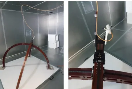
Fig. 1 : The robot optimized to weakly perturbate a
reverberation chamber in the GHz range. On the right, a detail showing the electro-optic probe.
First automated validation. Goals: a) to assess how
strongly the generated wavefronts contrast with the
diffusive background, b) they reproductibility and c) their
ability to generate spatially resolved EM stress.
-0.60 -40 -20 0 20 40 30 40 50 60 70 -0.14 -40 -20 0 20 40 30 40 50 60 70 0.60 -40 -20 0 20 40 30 40 50 60 70 -0.60 -40 -20 0 20 40 30 40 50 60 70 -0.14 -40 -20 0 20 40 30 40 50 60 70 0.60 -40 -20 0 20 40 30 40 50 60 70 -0.60 -40 -20 0 20 40 30 40 50 60 70 -0.14 -40 -20 0 20 40 30 40 50 60 70 0.60 -40 -20 0 20 40 30 40 50 60 70 -0.60 -40 -20 0 20 40 30 40 50 60 70 -0.14 -40 -20 0 20 40 30 40 50 60 70 0.60 -40 -20 0 20 40 30 40 50 60 70 -0.60 -40 -20 0 20 40 30 40 50 60 70 -0.14 -40 -20 0 20 40 30 40 50 60 70 0.60 -40 -20 0 20 40 30 40 50 60 70 -0.60 -40 -20 0 20 40 30 40 50 60 70 -0.14 -40 -20 0 20 40 30 40 50 60 70 0.60 -40 -20 0 20 40 30 40 50 60 70
Fig. 2 : Wavefronts sampled at three time instants over a vertical
plane, as they approach and leave the focal region (top to bottom): an example of local planar excitation (left column) and one limited by diffraction. -0.60 -40 -20 0 20 40 30 40 50 60 70 -0.60 -40 -20 0 20 40 30 40 50 60 70 -0.14 -40 -20 0 20 40 30 40 50 60 70 -0.14 -40 -20 0 20 40 30 40 50 60 70 0.60 -40 -20 0 20 40 30 40 50 60 70 0.60 -40 -20 0 20 40 30 40 50 60 70 -0.60 -40 -20 0 20 40 30 40 50 60 70 -0.60 -40 -20 0 20 40 30 40 50 60 70 -0.14 -40 -20 0 20 40 30 40 50 60 70 -0.14 -40 -20 0 20 40 30 40 50 60 70 0.60 -40 -20 0 20 40 30 40 50 60 70 0.60 -40 -20 0 20 40 30 40 50 60 70 -0.60 -40 -20 0 20 40 30 40 50 60 70 -0.60 -40 -20 0 20 40 30 40 50 60 70 -0.14 -40 -20 0 20 40 30 40 50 60 70 -0.14 -40 -20 0 20 40 30 40 50 60 70 0.60 -40 -20 0 20 40 30 40 50 60 70 0.60 -40 -20 0 20 40 30 40 50 60 70 -0.60 -40 -20 0 20 40 30 40 50 60 70 -0.60 -40 -20 0 20 40 30 40 50 60 70 -0.14 -40 -20 0 20 40 30 40 50 60 70 -0.14 -40 -20 0 20 40 30 40 50 60 70 0.60 -40 -20 0 20 40 30 40 50 60 70 0.60 -40 -20 0 20 40 30 40 50 60 70 -0.60 -40 -20 0 20 40 30 40 50 60 70 -0.60 -40 -20 0 20 40 30 40 50 60 70 -0.14 -40 -20 0 20 40 30 40 50 60 70 -0.14 -40 -20 0 20 40 30 40 50 60 70 0.60 -40 -20 0 20 40 30 40 50 60 70 0.60 -40 -20 0 20 40 30 40 50 60 70 -0.60 -40 -20 0 20 40 30 40 50 60 70 -0.60 -40 -20 0 20 40 30 40 50 60 70 -0.14 -40 -20 0 20 40 30 40 50 60 70 -0.14 -40 -20 0 20 40 30 40 50 60 70 0.60 -40 -20 0 20 40 30 40 50 60 70 0.60 -40 -20 0 20 40 30 40 50 60 70
Fig. 3 : Testing the wavefront repeatability after translation (left
column) and rotation (right column).
Observations: a) stable wavefronts against translation
and rotation, b) good level of contrast (> 20 dB), c) good
polarization control.
Applications : a promising application currently developed
is imaging coupling paths in metallic shields. An example
is shown below.
x (cm) z ( c m ) x excitation -20 0 20 -40 -30 -20 -10 0 10 20 30 40 -56 -54 -52 -50 -48 -46 -44 -42 -40 -38 x (cm) z ( c m ) z excitation -20 0 20 -40 -30 -20 -10 0 10 20 30 40 -56 -54 -52 -50 -48 -46 -44 -42 -40 -38 x (cm) z ( c m ) x excitation -20 0 20 -40 -30 -20 -10 0 10 20 30 40 -56 -54 -52 -50 -48 -46 -44 -42 -40 -38 x (cm) z ( c m ) z excitation -20 0 20 -40 -30 -20 -10 0 10 20 30 40 -56 -54 -52 -50 -48 -46 -44 -42 -40 -38Fig. 4 : A transmission image of a slotted metal box, showing the
position of a slot and its sensitivity to polarization. Moving focal spots were used in order to generate it.