HAL Id: halshs-02658784
https://halshs.archives-ouvertes.fr/halshs-02658784
Preprint submitted on 30 May 2020
HAL is a multi-disciplinary open access archive for the deposit and dissemination of sci-entific research documents, whether they are pub-lished or not. The documents may come from teaching and research institutions in France or abroad, or from public or private research centers.
L’archive ouverte pluridisciplinaire HAL, est destinée au dépôt et à la diffusion de documents scientifiques de niveau recherche, publiés ou non, émanant des établissements d’enseignement et de recherche français ou étrangers, des laboratoires publics ou privés.
Top Wealth Shares in the UK over more than a Century
Facundo Alvaredo, Anthony Atkinson, Salvatore Morelli
To cite this version:
Facundo Alvaredo, Anthony Atkinson, Salvatore Morelli. Top Wealth Shares in the UK over more than a Century. 2017. �halshs-02658784�
World Inequality Lab Working papers n°2017/2
"Top wealth shares in the UK over more than a century."
Facundo Alvaredo, Anthony B. Atkinson, Salvatore Morelli
Keywords : Inequality; inequality dynamics; top income; wealth share; DINA;
Distributional National Accounts; United Kingdom
Top wealth shares in the UK over more than a century
*Facundo Alvaredo
Paris School of Economics, INET at the Oxford Martin School and Conicet
Anthony B Atkinson
Nuffield College, London School of Economics, and INET at the Oxford Martin School
Salvatore Morelli
CSEF – University of Naples “Federico II” and INET at the Oxford Martin School
This version: 19 December 2016 Abstract
Recent research highlighted controversy about the evolution of concentration of personal wealth. In this paper we provide new evidence about the long-run evolution of top wealth shares for the United Kingdom. The new series covers a long period – from 1895 to the present – and has a different point of departure from the previous literature: the distribution of estates left at death. We find that the application to the estate data of mortality multipliers to yield estimates of wealth among the living does not substantially change the degree of concentration over much of the period both, in the UK and US, allowing inferences to be made for years when this method cannot be applied. The results show that wealth concentration in the UK remained relatively constant during the first wave of globalization, but then decreased dramatically in the period from 1914 to 1979. The UK went from being more unequal in terms of wealth than the US to being less unequal. However, the decline in UK wealth concentration came to an end around 1980, and since then there is evidence of an increase in top shares, notably in the distribution of wealth excluding housing in recent years. We investigate the triangulating evidence provided by data on capital income concentration and on reported super fortunes.
JEL Codes: D3, H2, N3
Keywords: wealth inequality, estates, mortality multipliers, United Kingdom, United
States
* Tony sadly passed away on January 1st, 2017, after the completion of this paper, which received
clearance from HMRC for public releasing on January 3rd, 2017. The paper entirely reflects our
joint views, discussions, and effort. We are and will be deeply indebted to Tony.
We acknowledge financial support, at different stages, from the Institute for New Economic Thinking (F. Alvaredo, A. B. Atkinson and S. Morelli), the European Research Council (F. Alvaredo through ERC Grant 340831), ESRC/DFID (F. Alvaredo through grant ES/I033114/1), and the University of Venice Ca’ Foscari “Guido Cazzavillan Fellowship” (S. Morelli). During the final phase of the project, S. Morelli was visiting fellow at the Center for Equitable Growth (University of California Berkeley) and the Employment, Equity, and Growth Programme at INET Oxford. We thank for helpful comments Arthur Kennickell, Brian Nolan, Thomas Piketty, Emmanuel Saez, Tony Shorrocks, Gabriel Zucman, as well as participants at the Conference on household wealth data and public policy (IFS and Bank of England, London, March 2015), the International Inequalities Institute Annual Conference (London, May 2016), the Third Annual Conference of the Society for Economic Measurement (Thessaloniki, July 2016), and the INET at Oxford seminar (November 2016). We are particularly grateful to Edward Zamboni and Andrew Reeves of HMRC, to the HMRC personal wealth statistics team, and to the Datalab staff for providing access to the UK Inheritance Tax microdata. Contact: alvaredo@pse.ens.fr.
1. Introduction: The distribution of personal wealth
Economists have recently focused on the distribution of personal wealth. There have been two main sources of impetus. One is the recognition of the importance in macro-economics of assets and liabilities, as demonstrated by the investments being made in launching household financial surveys, and by the renewed interest in balance sheets in national accounts. Another impetus has come from Thomas Piketty’s Capital in the
Twenty-First Century, in which he warned that the main driver of inequality – the
tendency of returns on capital to exceed the rate of economic growth – today threatens to generate extreme inequalities. The debate generated by this book has turned the spotlight on the empirical evidence concerning the upper tail of the wealth distribution, and the importance of historical time series. As Kopczuk has underlined, “estimates of the top wealth shares are much less settled than those of the top income shares, and there is substantial controversy about how they have evolved in recent years” (2016, page 2).
This paper presents new long-run evidence about top wealth shares – which we believe to be essential in understanding the evolution of the modern economy - for the United Kingdom (UK). It builds on the earlier line of research, summarized in Atkinson and Harrison (1978), and on the work of the official statisticians in Her Majesty’s Revenue and Customs (HMRC), but has a different point of departure: the distribution of estates left at death, recorded in the administrative data required for estate taxation and the administration of estates. The evidence covers an extensive period, starting in the “Gilded Age” before the First World War. The long-run results since 1895 highlight the enormous transformation of the distribution of wealth within the UK over more than a century. Figure 1, previewing the main estimates, shows that in the wake of the first modern globalization the share of personal wealth going to the wealthiest 1 per cent of UK individuals remained relatively stable at around 70 per cent. The share began to fall after 1914 and the decline continued until around 1980, when the share had decreased to some 16 per cent. This is still 16 times their proportionate share, but represents a dramatic reduction. The fall, however, came to an end around 1980, and since the mid-1980s the share of the top 1 per cent – representing approximately half a million individuals today – has moved in the opposite direction.
What lies behind the long-run estimates for the UK presented in Figure 1? The paper describes the three main methodological steps. Our investigation begins in Section 2 with the estimation of the distribution of estates from the administrative tax data, which covers the longest period of time under investigation (1895 to 2013). As a second step, in Section 3, we estimate wealth concentration applying the mortality multiplier method to the estate data. In the UK, this involves piecing together data for the different years when sufficient information exists on the demographic structure of estates to implement such method. It also means confronting the discontinuity introduced from 2005 when the HMRC ceased publication of the previous official series and adopted a new methodology. In Section 4, we link the different estimates of wealth concentration over time in order to provide a continuous time series from 1895 to 2013. The results cover, in addition to the evolution of top wealth shares, the shape of the upper tail, which builds a bridge with the theoretical literature on thick tails of the wealth distribution (see Benhabib and Bisin, 2016, for a recent review). We pay
particular attention to the role of housing in understanding the dynamics of wealth concentration. The new estimates represent, we believe, an advance on those available to date, but they should be viewed in the context of a variety of potential sources of error, arising both from the underlying method and from the reliance on tax data. In Section 5, we consider the internal validity of the estimates presented here by addressing the main problems with the methods used in their construction, and in Section 6 we apply checks on their external validity through an examination as to how far they can be triangulated with evidence from other sources.
Source: Table G1.
The new evidence about top wealth shares for the UK is compared in Section 7 with the evidence for top wealth shares in the United States (US). There has long been interest in contrasting wealth distributions in the UK and the US (for example, Lydall and Lansing, 1959, and Lampman, 1962). The juxtaposition of the two countries is of particular relevance given the recent critical reviews of the long-run US evidence (Kopczuk, 2015 and 2016, and Sutch, 2015), and the publication of alternative estimates by Bricker et al, 2016, and Saez and Zucman, 2016, the latter finding a particularly sharp rise in the very top wealth shares. Comparisons made half a century ago found wealth to be more concentrated in England, but today the US is seen as the home of major concentrations. If so, when did the countries change position? There are significant differences in the nature of the estate data – in coverage and in the process of assembly – but the sources are sufficiently similar to make the comparison a meaningful one.
In the final Section 8, we summarize the main findings and discuss the implications for the future measurement of the distribution of wealth (see also Alvaredo, Atkinson and Morelli, 2016).
Measuring the distribution of wealth
The paper is concerned with the distribution of personal wealth, or net worth: the value of the assets owned by individuals, net of their debts. Assets include financial assets, such as cash, bank accounts or bonds or company shares, and real assets, such as houses and farmland, consumer durables, and household business assets.
The total wealth considered here differs in important respects from total national wealth, as measured in the national accounts balance sheets. To begin with, we are concerned only with one sector of the economy: the household sector (sector S14 in the national accounts), where this excludes non-profit institutions serving households (sector S15). Secondly, there are differences in the method of valuation, a subject that is often neglected. The balance sheets are in principle based on values observed in the market, but it is necessary to distinguish between “realization” and “going concern” valuations (Atkinson and Harrison, 1978, page 5). Here the nature of the data on individual wealth-holdings at our disposal means that we focus on the former: what a person could realize by the sale of all assets, net of liabilities. The going concern valuation could well be
higher than that recorded in the statistics.1 In the case of household contents (durables,
furniture, etc.), for instance, the price obtained on sale is likely to fall considerably short of the value to a continuing household (or the replacement cost). A less common, but quantitatively important, example is that of business assets, where the realization value is likely to be less than the valuation on “going concern” basis. As these examples illustrate, the move to a going concern basis would add to wealth at different points on the wealth scale. On balance, moving to a going concern basis is likely to reduce top wealth shares (see Atkinson and Harrison, 1978, pages 112-113), and this should be borne in mind in what follows
In adopting a realization basis, we are open to the charge of departing from national accounting practice. However, it should be noted that the official UK statement about the basis for the balance sheet valuation states that
“market value is an estimate of how much these assets would sell for, if sold on the market” (Office for National Statistics, 2016, Section 2).
This sounds more like a realization basis than a going concern basis. What is more, once we depart from observed market transactions, any estimate of what assets “would sell for” involves a number of speculative assumptions. This applies to a number of classes of assets, but is particularly the case with defined benefit pension rights, both private and
1 Although this is not invariably the case. In the estate statistics, life assurance policies on the life
of the deceased are valued at the sum assured, whereas in the hands of the living their value is less than this amount, whether valued on a going concern or a realization basis. It would be possible to make adjustments to the recorded amounts (see Atkinson and Harrison, 1978, pages 95-99), but this has not been done here. In the same context, no account has been taken of the cash withdrawal/surrender value of defined contribution pensions.
state, where there have been a series of official UK estimates, but these have been subject to substantial revisions (see, for example, Inland Revenue Statistics 1995, pages 124-125).
It has also to be remembered that we are concerned about the distribution of wealth not only on account of the potential consumption. Wealth conveys power. The realization basis may be seen as capturing the degree of direct personal control over resources that is one of the major reasons for interest in the concentration of wealth. If, as it has been expressed by Abraham, there is concern that “a growing share of income and wealth is controlled by households in the top 1 percent or top 0.1 percent” (2016, page 313), then it is reasonable to omit assets, such as pension rights, over which the individual has only
limited or no control.2
There are five main potential sources of evidence about the distribution of personal wealth:
1. Household surveys of personal wealth, such as the UK Wealth and Assets Survey,
conducted by the Office for National Statistics, or the Survey of Consumer Finance conducted by the Flow of Funds Unit of the US Federal Reserve, or the Household Finance and Consumption Surveys co-ordinated by the European Central Bank;
2. Administrative data on individual estates at death, multiplied-up to yield
estimates of the wealth of the living, as utilised in the UK by Her Majesty’s Revenue and Customs (HMRC, previously the Inland Revenue);
3. Administrative data on the wealth of the living derived from annual wealth taxes;
4. Administrative data on investment income, capitalized to yield estimates of the
underlying wealth;
5. Lists of large wealth-holders, such as the annual Forbes Richest People in America
List, or the Sunday Times “Rich List” for the UK, which has been compiled by Beresford
(1990, 1991 and 2006).3
For the UK and the US, the third source does not exist: there is no annual wealth tax. Sample surveys are relatively recent: the earliest in the UK and the US were carried out in the 1950s. The Rich Lists are even more recent: the UK Sunday Times list dates from 1989; the US Forbes list started in 1982. This means that long-run historical evidence has to make primary use of sources (2) and (4). The latter, the capitalization of investment income, has recently been revived in the US by Saez and Zucman (2016), and was the subject of research in the UK in the 1970s (Atkinson and Harrison, 1974 and 1978). However, as explained by Alvaredo, Atkinson and Morelli (2016), the data necessary to satisfactorily apply this approach in the UK are unfortunately less readily
available than in the US.4
The main focus of the paper is therefore on the use of estate data. Estates are not the same as the wealth among the living, but it turns out that the estate distribution provides a valuable point of reference.
2 Our estimates equally exclude “human capital” (the capitalized value of future earnings) and the
value of rights to state benefits in kind such as health care, education, etc.
3 In some particular cases, population census also provide evidence about the distribution of
personal wealth.
4 The application of the capitalization method in the UK, as well as a re-evaluation of its
2. The distribution of estates
The distribution of estates (the net value of property of a deceased person) has
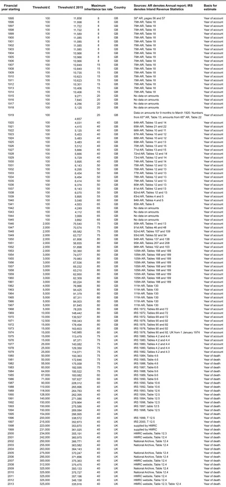
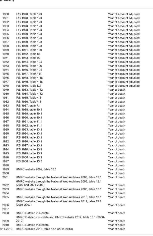
commonly served as a starting point for the estimation of the distribution of wealth among the living via the mortality multiplier method, but has never been under extensive scrutiny in and of itself. There are nonetheless reasons to consider the distribution of estates a good starting point, at least in the UK. First, there are tabulated data on the distribution of estates for almost all years from 1895 to 2013 (the missing years are 1915-1918, 1942-1945, 1995 and 2004). The sources of the estate data
are listed in Appendix Table A1.5 The estimates relate to Great Britain (excluding
Ireland) from 1895 to 1973, and the UK (including Northern Ireland) from 1974 onwards. This geographical definition reduces the extent to which the distribution is affected by the division of Ireland in 1921. The estates are taken to refer to adult deaths, where we take adult to mean throughout the period the population aged 18 and over (even though
the age of majority changed from 21 to 18 in 1970).6 The second main reason for
beginning with estates is that the underlying concept is relatively straightforward: it is the wealth left at death, and there is inherent interest in the concentration of inheritances. Thirdly, the estate distribution does not involve the multiplying-up process described in Section 3, and where the choice of mortality multipliers has been the subject of intensive debate.
Figure 2 shows the upper tail of the distribution of estates over the period from 1895 to 2013 (the underlying estimates are given in Appendix Table E1; the top shares in total
estates are interpolated from the published tabulations classified by ranges of estate
size).7 The changes in top shares may be summarized in terms of the three periods
marked by vertical lines in Figure 2. The first of these is the twenty-year period leading up to the First World War. There was a scarcely perceptible decline in the top shares: that for the top 1 per cent went from 69.2 per cent in 1895 to 67.3 per cent in 1914. The groups at the very top saw an actual increase in their share: that of the top 0.1 per cent rose from 31.8 per cent to 33.1 per cent, and that of the top 0.05 per cent from 23.9 to 25.4 per cent. The last of these figures means that the top 0.05 had more than 500 times their proportionate share of total estates. At the other end of the scale, the bottom 90 per cent had very little wealth at death. In short, estates were highly concentrated at the top, and there was overall little sign of change.
The second period covers more than half the twentieth century: from 1914 to 1980. This encompassed two world wars, and much attention has been paid to the loss of capital during the periods 1914 to 1918 and 1939 to 1945. Top shares certainly fell in the UK during the war years, but these only accounted for a part of the large reduction that took place over the period as a whole. The share of the top 1 per cent in total UK
5 The data are based on a sample, as described in Appendix I.
6 This definition follows that in the official Inland Revenue (IR)/Her Majesty’s Revenue and
Customs (HMRC) estimates of the distribution of wealth. At one point, the IR defined the adult population as those aged 15 and over (see, for example, Inland Revenue Statistics (IRS) 1976, Table 108), but with effect from IRS (1978) this was changed to 18 and over (see IRS 1978, page 79). Earlier studies of the distribution of wealth took those aged 20 and over (Lydall and Tipping, 1961) or even 25 and over (Daniels and Campion, 1936). On the grounds that there had been a downward trend in the age of economic independence, Atkinson and Harrison (1978) took a cut-off that began at 23 in 1923 and then fell by 1/10th of a year until reaching 18 in 1972.
estates fell by 48.7 percentage points between 1914 and 1979, but the war years only contributed 10.5 percentage points. The share of the top 0.1 per cent fell by 27.2 percentage points, but again only a quarter (6.2 percentage points) took place during the war years. The large decline in top shares was very much a peacetime phenomenon. The third period is from 1980 to the present. There have been year-to-year variations, but over the thirty years as a whole little change in top estate shares. The share of the top 1 per cent ended in 2013 at virtually the same figure as in 1980. The share of the top 0.5 per cent was higher by 1 percentage point, but that of the top 5 per cent was lower by 1.5 percentage points.
Source: Table E1.
The nature of estate data
The estate data are important both in their own right and because they provide the basis for the estimation, using the mortality multiplier method, of the wealth of the living discussed in the next section. The existence of the data reflects the institution of a single Estate Duty in 1894, substituted in 1975 by the Capital Transfer Tax, which was in turn replaced by the Inheritance Tax (IHT) in 1986, currently in place. The data derive
from the legal process of administering the estate of a deceased person, which is a
distributed according to the will or according to the legal provisions in the case of the person dying intestate. Before allowing an executor (usually indicated within the will) to administer the estate, a Court has to validate and prove the will (granting probate). This legal process of probate defines the true definitive testament of the deceased person and, in doing so, provides (often professional) assessments of estate valuation.8
The latter are then used to submit the IHT form in order to work out if any tax needs to be paid. After submitting the form (required within one year from the death), the executor or the administrator of the estate needs to swear an oath stating that the information given is true and accurate. It is after this process that usually the court issues a Grant of Representation (known as confirmation in Scotland and probate in the rest of the UK).9
Not every estate needs a Grant of Representation by the Probate Registry. In particular, a grant is not required for assets below the probate limits (currently £5,000), or for assets above the probate limit held jointly and therefore passing automatically to the other joint owner (e.g. a surviving spouse or civil partner).However, assets for which a grant of representation is not required are still recorded in our data to the extent that the estate of the deceased also includes assets for which a grant of representation is needed.
As a result, the estates identified in our data, referred to as the “identified” estates,
cover only a fraction of all deaths in a year (see Appendix Figure C1), currently around a half. Therefore, an estimate of the total value of estates including those not covered by the estate returns, referred to here as the “excluded estates”, is required to derive top estate shares. The need to estimate the amount of “excluded wealth” is an important limitation of the estate method. At the same time, on the plus side, it is evident from the description given above that the valuation of the identified estates is the result of a much more thorough process than is likely to be carried out when collecting wealth data in other forms.
The derivation of the estate total
The total of estates is taken as the sum of the identified total in the estate returns plus an estimate of the total of excluded estates. The latter is in turn calculated from the estimated total wealth excluded from the wealth estimates described in the next section, by making the assumption that the amount of excluded estates passing in a year is given by the mortality rate of the excluded population (the ratio of deaths among the excluded population to the total number of living persons in that population) times the excluded wealth. In other words, it is assumed that the average wealth of the dying among the excluded population is equal to the average for the living in that population. Such an assumption would not be appropriate if applied to estates as a whole – as we
8 According to the National Audit Office Report on Inheritance Tax (2004), professionals are engaged in around 70 per cent of cases of probate.
9The linkage with the probate system significantly reduces the risk of the non-filing of tax returns in the UK (see National Audit Office, 2004, page 25). On the contrary, probate is obtained before paying the Federal Taxes in the United States.
discuss in the next parts of the paper – but may not be unreasonable as a first
approximation when applied to a group whose wealth is by definition limited.10
Beyond the estimation of the value of the excluded estates, there are a number of criticalities with the use of the estates statistics, which are discussed in later sections.
3. The distribution of wealth based on the estate multiplier method
The distribution of wealth of the living is conceptually different from that of the decedents. Death does not “sample” randomly the population. Older individuals, as well as males and people from poorer backgrounds, have, other things being equal, higher mortality risk. Differential mortality multipliers can however be used to transform the estate data into estimates of wealth-holding. Under the assumption that death is random within specific cells of observed demographic and social strata, one can view death occurrence as an effective sampling of the living population.
The inverse of the death rate, and hence the mortality multiplier, varies considerably with age: for example, in 1968 the general mortality multiplier for men varied from 3.74 for those aged 85 and over to 1102.18 for those aged under 25. Applying such differentials could be expected to lead to a distribution of wealth that differs a great deal from the distribution of estates. The impact could be expected to be further affected by the use of multipliers that reflect the lower mortality of the wealthy. In the UK, the assumption was initially made that wealth was correlated with social class as defined by occupational categories, and later refined by the introduction of variables such as marital status, home ownership and housing wealth. In what follows, we make use of the official (IR/HMRC) estimates of identified wealth for the period from 1960 and hence accept their choice of multipliers. For much of the period, the official multipliers have been differentiated according to gender, age group, country (England and Wales, and Scotland, in the case of Great Britain), and estate size class. For the period before 1960, we apply the social class mortality multipliers employed in Atkinson and Harrison (1978, Chapter 6) based on occupational classes, where these vary by decade.
The application of the available mortality multipliers to the pre-1960 estates data, and the use of available multiplied tabulations by wealth ranges since 1960, yields estimates of the distribution of identified wealth covering 1911 to 2012:
a) for the years 1923 to 1930, 1936, 1938, and 1950 to 1959, tabulations of estates by ranges broken down by age and gender are available, and we apply mortality multipliers and social class adjustment factors to make estimates of identified wealth by ranges (the sources and coverage are listed in Atkinson and Harrison, 1978, Table 6.3); there are in addition tabulations by age and estate size, but not gender, for the years 1911-1914,
10 A check on the assumption is provided by calculating the implications for the overall ratio for
the whole population (included and excluded) of the average wealth of decedents to the average wealth of the living. The values in the early part of the period are around 2, falling to 1.5 in the 1950s. These do not seem unreasonable. Moreover, the fact that, until 1975, the values are considerably above those found by Piketty (2011) in the case of France suggests that the allowance should not be increased (see Appendix Figure C4).
and 1920, and we have also made use of these.11 Estimates derived for the years 1938-1959 refer to Great Britain whereas the pre-1938 period refers to England and Wales. b) for the period 1960 to 2005, we rely on the published tabulations (IR/HMRC) of identified wealth-holdings by ranges (see Appendix Table A2 for sources); the IR/HMRC applied social class multipliers, varying by age, sex and country; in the course of the period, the IR/HMRC switched from using statistics for the valuation of the estate on a year-of-account basis (the date at which the estate was administered) to using statistics
on the more appropriate year-of-death basis.1213 The data for the period between 1960
and 1973 refer to Great Britain, whereas the data from 1974 refer to the UK. These wealth tabulations were used by the IR/HMRC to derive their first “official” estimates of the distribution of wealth in Great Britain from 1960, later referred to as Series A (not covering the excluded population, and therefore of little utility), and Series B (covering the excluded population but with no allowance for the wealth of the excluded population). These estimates were the subject of detailed examination by the Royal Commission on the Distribution of Income and Wealth (1975 and subsequent reports) and by Atkinson and Harrison (1978). Subsequently, the Inland Revenue introduced a Series C that makes adjustments for the wealth of excluded population. This Series C was revised in 1984 (Inland Revenue Statistics 1984, page 43) and continued to be published on an annual basis for years up to 2005 (see Table K1). In addition, the IR/HMRC Series C corrected for under reporting of the wealth of the included population and made adjustments to its valuation. In the research presented here, we are unable to make these additional adjustments, as the underlying data cannot be made available to us. c) for the grouped years 2001-03, 2005-07, 2008-10, and 2011-2013, we use the new version of the tabulations of identified personal wealth-holdings published by the HMRC; these differ in that, in addition to the grouping of years, the HMRC uses a revised methodology to capture the negative correlation of mortality with (housing) wealth and to apply lower mortality to smaller estates; the results for 2001-03 provide an overlapping observation that is used to link the series (and, in Section 5, to investigate the implications of the change in methodology).
d) differently from other years, for the three years 2008, 2009 and 2010, we have made use of microdata available from the HMRC Datalab, where the data set has been designed so as to ensure anonymity and protect taxpayer confidentiality.
The derivation of the wealth total
The wealth holdings identified by the multiplier process have to be compared with the control total for the population as a whole. The control totals for wealth (and for total
11 For years when estates are not broken down by gender, the social class differential is taken as
2/3 of the male plus 1/3 of the female.
12 The distributions by range of wealth from 1960 onwards were collected for a number of years in
the first edition of Inland Revenue Statistics in 1970, the numbers in earlier years being revised from the previous publications. These numbers have been used for the years 1960 to 1968.
13 The IR continued for a number of years to publish the distribution of estates by age and sex of
the deceased (for example, Table 112 in Inland Revenue Statistics 1970), but these contain less detail than was available to the IR in making their estimates, and we have therefore relied on their multiplier process.
population) are given in Table D1. To arrive at the wealth control totals, we employ the national balance sheets, but it should be stressed that the control totals are not necessarily equal to the balance sheet totals for the personal sector. It is not simply a matter of replacing the total by one drawn from the published national accounts. Among the major reasons for the difference is the inclusion in the official UK balance sheets of the value of private pensions, which do not fall within the definition of personal wealth
adopted here.14 A further example is provided by the issue of timing. The balance sheet
figures refer to a point in time (31st December); the estate data refer (now) to the date of death. The latter seems appropriate, and there is no reason to make the “end-year
adjustment” incorporated in the balance sheets.15
As part of the research carried out by the IR/HMRC, they have, beginning with IRS 1980, published tables on the “Reconciliation of estate multiplier and balance sheet estimates”. The aim is to explain the relationship between Total Identified Wealth, obtained by multiplying up the estate data by mortality multipliers, and the information available from external sources, drawing on the national balance sheets. Such a reconciliation exercise was a major development with regard to estimates of the distribution of wealth since it allows for
i) the wealth of the excluded population;
ii) differences in coverage/valuation (including under-recording) for which we would
like to adjust the totals employed when calculating the shares of top wealth groups;
iii) differences in coverage/valuation for which adjustments should be made to the
ranges of wealth identified in the estate-based estimates.
In 2005, the last year for which the exercise has been published, the total identified wealth is £3,432 billion, to which is added £908 billion (26 per cent) for the wealth of the excluded population (including in this case omitted wealth held in trusts). A similar amount (£826 billion) is added for under recording, and £161 billion is subtracted to allow for differences in the valuation (such as in life policies). The end result of these adjustments – stages i), ii) and iii) – is total marketable wealth (this is the so called Series C total), which is £5,005 billion, or 46 per cent higher than total identified wealth - see Figure 3. The Series C total is considerably less than the total national balance
14 A further element is that the balance sheet total for the personal sector includes Non-Profit
Institutions Serving Households (NPISH), such as sports clubs, churches, universities, and trade unions. In recent years, they have accounted for some 2 per cent of the balance sheet total (HMRC website 2005, Table 13.4) and this should be deducted. The national accounts definition of total personal net worth does not include consumer durables. It also differs in adding an end-of-year adjustment. In earlier years, the national accounts included the value of non-marketable tenancy rights (intangible assets including housing and agricultural tenancy rights), but from the 2012 edition of the national accounts and to be aligned to the European System of Accounts 1995, “non-marketable tenancy rights” have been excluded, reducing net worth in 2005 by £487 billion.
15 On the other hand, in earlier years the IR data referred to the date at which the estate was
administered (“year of account”). Since the period of administration varied considerably, the deaths in question could have occurred in another calendar year: IRS 1980 says of the 1976 year of account data that “while the figures related in the main to deaths in 1976, also included were details of estates where death occurred earlier than 1976, and in a few cases in the first quarter of 1977” (p. 101). This may make quite a difference where asset prices are changing rapidly, and when linking the series allowance is made for the potential difference. It should also be noted that the lengthy process of administration may lead to the IR/HMRC making revisions to the data. For example, revisions to the identified wealth tables for 2002 published by HMRC in 2010 led to a 2 percentage point rise in the wealth share of the top 10 per cent (although a much smaller change in the shares of the top 1 and 0.1 per cent).
sheet figure for the wealth of the personal sector, including an estimate of the value of
funded private pension rights, which in 2005 was (excluding NPISH) £6,292 billion.16
Since the adjustments (ii) and (iii) cannot be carried back in time, we have given priority to consistency over the full historical period from 1895 to 2005. This means that the series of control total wealth in our paper adds the estimates of total identified wealth
and the estimated wealth of the excluded population.17 The addition for the excluded
population is necessary, since, as explained above, not all assets and possessions come to notice to tax authorities. In the tax year 2005-6, for example, there were 273,043 estates included in the statistics for the UK, compared with a total of 577,113 adult deaths (see Appendix B for sources). When multiplied up to give an estimate for a point in that year, the resulting number of identified wealth-holders fell considerably short of the total adult population: 18.7 million identified wealth-holders compared with an adult population of 47.1 million. Therefore, for 2005-6, it is necessary to make an
addition to total wealth for that owned by the excluded 28.4 million.18
The starting point for our estimates of the wealth of the excluded population is the set of estimates that were made regularly by the HMRC as part of their reconciliation exercises. These show from 1975 to 2005 (and for 1971) the estimated totals under the headings “small estates” and “joint property” (we do not include omitted property held in trusts). Joint property, typically an owner-occupied house, has always been the larger part of the total wealth of the excluded population, but the ratio of joint property to the remainder has changed from around 2:1 in the 1970s to 10:1 in the 2000s. For earlier years before 1971, we make use of the estimates in Atkinson and Harrison (1978, page 305). As is explained in Appendix C, there are good reasons for supposing that in the period from 1950 to 1970 these earlier estimates are too low. For this reason, we employ the “higher” estimate, rather than the “central” estimate. These earlier estimates are supplemented for the period before 1923 by the series constructed in Atkinson (2013), with the 1895 figure being extrapolated from that for 1896 using the ONS Consumer Price Index. This series did not include jointly owned property, which was then much less important, and the series is increased proportionately by the ratio in 1923. The details of the estimation method are given in Appendix C.
For years beyond 2005, however, this approach cannot be followed, since this was the last year in which the HMRC made an official estimate of excluded wealth. There is therefore an inevitable hiatus in the series. It is true that we have estimates of the total identified wealth from the estate data (which have continued), and the approach closest to that employed up to 2005 would be to add this to a forward extrapolation of the 2005 total for the excluded population. As however is discussed further in Section 5, we have doubts about the identified wealth totals after 2005, and these spill over into any estimate of the excluded wealth total, which depends on both the size and composition of the group that does not appear in the estate statistics. For simplicity, we begin with an alternative approach, using the year-to-year variation of national accounts balance
16 When NPISH is added, the last item corresponds to the item “Total net worth” (item CGRC) in
Table 10.10 of the national accounts.
17 This was the basis adopted by Atkinson and Harrison (1978, Chapter 6), and Atkinson, Gordon
and Harrison (1989), in their long-run series on wealth concentration (reproduced in Table D1).
18 Differently from the case of the US where only approximately 1 per cent of estates are covered
by estate statistics, the substantial coverage of the decedent population in the UK allows the derivation of internal measures of total personal wealth.
sheet total for the personal sector. This is the basis for the series developed below, with the control total for 2005 being increased by the same proportion as the rise in the
national balance sheet total.19 We are therefore departing from our earlier practice in
employing an external control total – but only for the purpose of linking over time. For the reasons given above, this is not ideal; the UK balance sheet totals also include non-profit institutions serving households. In view of this, we revisit the assumption in the sensitivity analysis in Section 5. A second possibility is to use the personal wealth total (excluding private pension wealth) in the Wealth and Assets Surveys (WAS), taking account of the fact that these relate to interviews carried out over a 3-year period. These, however, show rather different patterns of change over time. The WAS totals show a 1 per cent fall between 2006-08 and 2008-10, whereas the national balance sheet shows a fall of 3.3 per cent; the WAS totals show a rise of 8 per cent between 2008-10 and 2010-12, whereas the balance sheet totals show a rise of 13 per cent. In the absence of a reconciliation of the totals provided by different sources, we employ the national accounts balance sheet figures, but, as discussed further in Section 5, the uncertainty surrounding the control totals limits what we can say regarding the changes in top wealth shares since 2005.
The resulting main series for total wealth per adult combining the identified wealth and the estimated wealth of the excluded population are shown in constant consumer price terms in Figure 4. There is year-to-year variation, but the average remained relatively stable for much of the first three-quarters of the twentieth century: average wealth in 1980 was little higher in real terms than in 1920. There followed a marked rise, with the average at the start of the twenty-first century being some 3 times that in 1980. The threefold increase is similar to that recorded by Kopczuk and Saez (2004a, Table A) for the US between 1916 and 2001, but the time path is quite different, since average wealth in the US had doubled between 1916 and 1980. Among the reasons for the difference are the impact in the UK of house price booms and the spread of owner-occupation, and the transfer of wealth to the personal sector from the public sector as a result of the privatization of state enterprises and public housing. We return to the role of housing below. Figure 4 also compares the series used here – the sum of identified wealth and the wealth of the excluded population – with our attempt to construct from 1911 a “marketable wealth” series comparable with the HMRC Series C (the methods are described in Appendix D). As is to be expected, the marketable wealth series lies typically, but not universally (the adjustments may be negative) above our main series, but the time pattern is close.
Source: Table D1 and HMRC website.20 Source: Table D1. 20 Table 13.4 in http://webarchive.nationalarchives.gov.uk/20101006170448/http://hmrc.gov.uk/stats/personal _wealth/menu.htm
4. Towards a long-run series for top wealth holdings in the UK
The results of the multiplier process, combined with the control totals, provide estimates of the top shares. As is inevitably the case with such a long time series, its construction involves the linking of estimates on different bases across time. There are seven potential breaks in our estimates:
A) at 1923 which is the first year for which we have estate data broken down by gender, as well as age and estate class;
B) in 1938 when the data begin to cover Great Britain in place of England and Wales; C) in 1960 when the IR began to use the estate data to make wealth estimates;
D) in 1974 when the data begin to cover the United Kingdom in place of Great Britain; E) in the 1970s and 1980s when there is a switch from a year of account basis to a year of death basis;
F) after 2002 when HMRC introduced a new methodology for wealth estimation and the “New HMRC Estimates”;
G) 2008-2010 when it became possible to use a form of micro data from the HMRC Datalab.
The different elements are summarized in terms of their implications for the share of the top 1 per cent in Figure 5. Of the seven, the element G should not in principle lead to any discontinuity (although we have drawn attention to the fact that the data in fact aggregate estates, which may lead to the results differing from those from the full micro data). In what follows, we consider the different potential breaks A-F, taking the post-2002 series as the point of reference, following the national accounts practice where estimates on earlier bases are revised to bring them into line with the most recent methodology.
First, there is geographic coverage. The earlier series constructed by Atkinson and Harrison (1978) showed a break for geographical coverage between 1938 (England and Wales, EW) and 1950 (Great Britain, GB). The differences are however small, as may be seen by comparing estimates on the two bases for 1938 to 1972 in Figure 5. For the top 1 per cent share, the maximum difference between the EW and GB estimates is 0.6 percentage points and for half the years the difference is 0.2 percentage points or less. We therefore treat the series as continuous at 1938. In the same way, the change to a UK basis in 1974 is assumed not to have materially affected the estimated top shares (the added population, that of Northern Ireland, is 2.9 per cent of the UK total).
Source: see Table G3.
The breaks B and D are therefore not further discussed. This leaves four breaks where the series have to be linked. The first of these concerns the use of gender-specific multipliers. Substituting multiplier number and wealth values with their respective weighted average by gender components in 1923 and 1924, yielded differences between the share of top 1 per cent with and without gender tabulation of respectively 0.7 and 0.5 percentage points. This suggests that we should reduce the pre-1923 figures in each case by 0.7 percentage points, on the assumption that the difference is additive.
The next break is that in 1960. The earlier series constructed by Atkinson and Harrison shows a major break in continuity in 1960 (a break that has typically been ignored by users of the data), with the share of the top 1 per cent being lower by some 7 percentage points (1978, Table 6.5). This was based on the a priori grounds that there had been major changes in 1960 in the estate data available to the Inland Revenue: from that date, the data included estates below the tax threshold which nonetheless came to the notice of the Inland Revenue when a grant of representation was obtained. The underlying data became more complete, and it is also possible that the decision to prepare official estimates of wealth-holding from that year may have led to the estate statistics being collected with more care than in the past. The effect in terms of coverage may be seen from the fact that the statistics, when multiplied up, covered 17.9 million taxpayers (48.5 per cent of total adults), compared with 3.1 million with wealth above the threshold (£3,000) who were only 8.4 per cent of adults in 1960. As noted earlier, there are good reasons to suppose that for early part of the post-war period the allowance made by Atkinson and Harrison (1978) for the property of the
Back to index 0 10 20 30 40 50 60 70 80 1910 1915 1920 1925 1930 1935 1940 1945 1950 1955 1960 1965 1970 1975 1980 1985 1990 1995 2000 2005 2010 2015 Sh ar e o f to ta l p er so n al w ea lth %
Figure 5. Piecing together different series for the UK top 1%
wealth share 1911-2012
EW: no gender
EW: gender available
GB
UK: year of account
GB: IR estate-based UK: year of death New HMRC methodology UK: micro data
excluded population was too low, under-estimating the value of joint property. This has been corrected, which reduces the downward jump in top shares (it is now 5 percentage points). Since there are no years of overlap, with estimates on different bases, there is no direct method of linking the series. However, as we argue in the next section, the data on estates are informative. Between 1959 and 1960, the estimated share of the top 1 per cent in estates fell from 34.72 per cent to 33.67 per cent. We have assumed that the difference of 1.05 percentage points represented the genuine change between the two years in the wealth shares, and linked the earlier wealth series on that basis (with
corresponding assumptions for other wealth groups).21
For the remaining two breaks, we have estimates for overlapping years, and these form the basis for the linking. We have used the IR estimates on a year of death basis from 1978 onwards, adjusting the earlier year of account estimates by the difference in the estimated wealth shares in 1985 (an overlapping year, and one where the new estimates appear to have settled down). (The sensitivity to the choice of overlapping year is discussed below.)
Finally, there is the break associated with the adoption of a new methodology from 2002. The most important changes are the application of new multipliers and the adoption of a new sampling strategy of the estates population (HMRC, 2012). Since the latter was associated with a smaller sample size, the HMRC moved to producing estimates based on data averaged over three years (2001-2003, 2005-2007, and 2008-2010) in order to reduce sampling variation. We note that the HMRC has stated that “the overlap between the historical data and the new time period would allow users to construct a time series bearing in mind the limitations and changes to the methodology” (HMRC, 2012, page 16). However, in the main series we have adjusted the estimates prior to 2002 additively by the difference between the New HMRC Estimates for 2001-03 and those obtained for 2002 with the old methodology. In Section 5, when discussing the sensitivity of the estimates, we return to the problems surrounding the new methodology and the post-2000 wealth shares, and give an alternative set of estimates for the most recent years.
To sum up, although marginal in magnitude on average, we have made four additive adjustments in the course of linking the series, designed to bring them into line with the reference series for the most recent years.
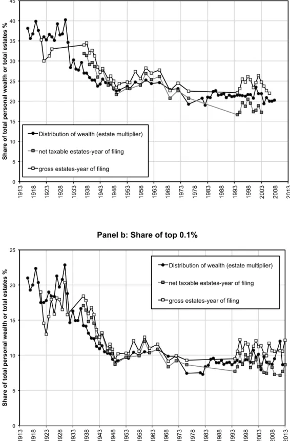
Comparison of the distributions of estates and of wealth
The series for the distribution of wealth is now brought together with that for the distribution of estates described in Section 2. Figure 6 compares the shares of the top 1 per cent for the two series. Theoretically, the application of multipliers embedding differential mortality by age and wealth can increase or decrease wealth shares as well as change the time pattern (relative to estate shares), depending on the evolution of the age-wealth profiles. When the age multiplier method was first employed in the UK, it was seen as overcoming a “fatal” objection to the use of estate data, since “the accumulated wealth of an individual increases with years … and is usually greatest when
21 The 1959 estimates do not extend down to the top 10 per cent, so that the absolute difference
a man dies” (Mallet, 1908, page 67). Our findings suggest that the objection is in fact less than fatal. In practice, for much of the period the conclusions reached regarding the degree of concentration do not change radically. As shown in section 7, such a
result carries through to the US; it also applies to 19th century Paris, (Piketty,
Postel-Vinay and Rosenthal, 2006). The similarity of the movement over such long periods in the three cases may be seen as a surprising finding. However, it can be proved that the effect of multipliers on the move from estates to wealth is such that the estimated distribution of wealth exceeds that of estates by a covariance term between the multiplier and the level of estates, where this covariance is likely to be positive. This has the same mathematical form as the impact of rates of return on the move from investment income to wealth.
The exception to the conclusion just described concerns the most recent years, when Figure 6 shows the wealth series as rising relative to the estate series after 2002, the wealth estimate of the share of the top 1 per cent exceeding the corresponding share for estates by an average of 5 percentage points. This departure may be explained by the limitations of the method used to construct a control total for wealth post-2005, but we believe that it also occurs on account of the changes in multipliers, as part of the changes in methodology adopted by the HMRC since 2002. We return to this in Section 5.
Source: Table E1 and Table G1.
The close relationship between estate distribution and wealth distribution provides a useful measurement benchmark in order to extend the wealth concentration series back in time to 1895, and to fill in missing years especially in the earlier years of twentieth century. More precisely, we apply the approach to interpolation and extrapolation proposed by Friedman (1962) involving the use of related time series. In the present case, we use the estate series to interpolate the gaps between available observations of top wealth shares. The relationship between top wealth shares and top estate shares,
estimated from 1911 to 2005 by ordinary least squares, is shown in Table 1.22 The
predicted values are then used to provide estimates of the top wealth shares for years that are missing from the wealth series from 1895 to 2005. The final series are shown in Figures 7a and 7b, and full results are given in Table G1. Figures for the share of top 1 percent of total wealth are those illustrated in Figure 1 in the introduction. The remaining gaps are those years for which there are no estate data, mostly during the war years.
Table 1 Linear regression of wealth shares on estate shares 1911-2005
22 We have examined the sensitivity of the estimates to the use of semi-parametric or local
non-parametric regressions. For our semi-non-parametric exercise, we used Robinson's (1988) double residual estimator and estimated the nonlinear relation between top estates shares and top wealth shares using a Gaussian kernel weighted local polynomial fit. Our non-parametric findings were based on a locally weighted regression of top wealth shares on estate shares (with running-line least-squares smoothing). It turns out that predicted values of top wealth shares on the basis of these different approaches track each other closely and that our estimates appear quite robust.
[1] [2] [3] [4] [5] Top 10% share (wealth) Top 5% share (wealth) Top 1% share (wealth) Top 0.5% share (wealth) Top 0.1% share (wealth)
Top 10% share (estates) 0.937*** (0.010)
Top 5% share (estates) 0.965***
(0.008)
Top 1% share (estates) 1.006***
(0.009)
Top 0.5% share (estates) 1.005***
(0.012)
Top 0.1% share (estates) 1.066***
(0.023)
Constant 2.608*** 0.846 0.337 0.636 0.451
(0.699) (0.488) (0.337) (0.328) (0.374)
R-squared 0.993 0.995 0.994 0.991 0.974
Observations 58 68 68 68 60
Notes: Table based on linear regressions of top wealth shares series on the respective top estate shares measured in percentage points. The sample used is 1911-2005 (included). Standard errors in parentheses.
* denotes p<0.05. ** denotes p<0.01. *** denotes p<0.001.
The distribution of wealth from 1895 to 2013
What does the final series show? The estimated top wealth shares before the First World War were very high. The share of the top 0.1 per cent was at least one third, which meant that they had more than 333 times their proportionate share. The share of the top 1 per cent was around 70 per cent, and that of the top 5 per cent around 90 per cent. In particular, it is worth noting that recorded wealth concentration was high despite the lack of correction for settled property; Daniels and Campion (1936, page 39) estimate that 15 to 20 per cent of the settled capital passing at death was excluded from the estate duty returns in 1911-13, compared with a much smaller figure (4 to 7 per cent) in 1924-30. If a substantial amount of settled property was missing from the estate duty statistics for the years 1911 to 1914, then the top shares may be significantly
under-stated.23 After 1914, the top shares then began to fall, with the rate of decline
accelerating after the Second World War. By 1979 the share of the top 1 per cent, which had been around three-quarters, was closer to one-fifth. The share of the top 0.1 per cent, which had been a third, was by 1979 around 7 per cent. By any standards, this represents a dramatic reduction in wealth concentration over two-thirds of a century. Panel b of Figure 7 demonstrates the importance of looking within the top 10 per cent. The share in total wealth of those in the top 10 per cent, but not in the top 1 per cent (i.e. the “next 9 per cent”) saw a rise in their share for the first half of the twentieth century, followed by a period of stability until the end of the 1970s. This underlines the changing shape of the upper tail, to which we return below.
Since 1980, the decline in top shares has come to an abrupt stop. The subsequent behaviour of the top shares is not easily summarized: it depends on the period considered and on the part of the upper tail on which one focuses. The reader of the official report UK Personal Wealth Statistics 2011 to 2013 is told that over the ten year period 2001/03 to 2011/13 “the distribution of wealth held by each decile has been broadly unchanged” (HMRC, 2016, page 4): the conclusion is one of stability. However, this distribution relates only to those identified as wealth-holders, and no account is taken of the existence or wealth of the excluded population. Moreover, grouping in terms of deciles is too crude to capture properly what is happening at the top. The estimates presented in panel a of Figure 7 suggest that the trend in the share of the top 1 per cent of all adults was upward. Moreover, panel b of Figure 7 shows that the experience was not uniform across top wealth groups. The lower half of the top 1 per
cent (those between the 99th and the 99.5th percentiles) saw a relative stability in their
share of total wealth, whereas the upper half saw an increase. It is not just the share of the wealthy that has changed but also the shape of the upper tail, to which we now turn.
23This was due to the fact that before 1914 where estate duty had been paid on settled property,
duty was not payable a second time the property passed. Daniels and Campion (1936) also show that the settled property reported in 1924 and 1925 rose as a proportion of total property from 7.0 per cent for estates between £100 and £1,000 to 21.7 per cent for estates over £100,000 (Table 14).
The shape of the upper tail
In seeking to understand further the evolution of wealth concentration, it is helpful to
consider the share, !!, of the top i per cent expressed as a multiple of their population
share, 1 − !!. The extent to which the wealth share exceeds the population share may
then be seen as the product of two components:
!
!1 − !
!=
!
!µ
! !
!where !! is the i-th percentile from the top, expressed relative to !, which is the overall
mean wealth, and !(!!) is the mean wealth above !! expressed as a ratio of !!. The
extent to which the top 1 per cent, say, have more than their proportionate share
depends, via the first term, on the wealth required to enter this group (!!/!), which we
refer to as the “entry price”. This may be seen as capturing the degree of skewness to the right. The second component is an indicator of the degree of concentration within the top i-th per cent, or of the thickness of the right tail. If all estates in the top i-th per
cent are equal to the i-th percentile, then !(!!) equals unity.24 But to the extent that
there is inequality within the top i-th per cent, !(!!) is greater than 1, and the second
component increases the top share. In the case of the Pareto distribution, with Pareto
coefficient α, !(!!) is a constant not dependent on !!, equal to β=α/(α-1), often taken
as a measure of concentration, and referred to as the inverted Pareto-Lorenz
coefficient.25
We begin with the entry price. For this element of the analysis, we consider the unlinked series, since the linking factors described earlier do not apply to percentiles, and, since we have not attempted to interpolate the percentiles, the decomposition is made only for years where the full wealth distribution has been estimated. This means that the series start in 1911. Again there is differing experience within the top 10 per cent. The “entry price” for the top 10 per cent and 5 per cent increased up to the end
of the 1970s, and then levelled off. At the other end of the scale, the 99.9th percentile
fell steadily up to the 1980s and then began to rise (Figure 8). Taking the period as a whole, we see that the top percentile (entry price for the top 1 per cent) has halved since 1914.
This evidence for changing shape is complemented by that for the second element: the degree of concentration within the top groups. The degree of concentration within groups is measured in Figure 9 by the values of β estimated from different “shares within shares”: for instance, the share of the top 1 per cent within the top 10 per cent.
If the distribution is Pareto in form, then in that case 1/β = log10[S10/S1].26 The results in
Figure 9 for different groups show that there was a modest decline in the extent of concentration before the First World War, affecting the top 10 per cent but not the very top 0.1 per cent. There was then a sharp fall in the degree of concentration at the top in the inter-war period from 1919 to 1939, followed by a continuing fall from 1946 to the
24 In principle, the external control total for the adult population allows us to define the
percentiles in £, and the m function can be calculated (it is unit-free).
25 The ! function is related to the mean excess function, or mean residual life function, used in
actuarial science and risk analysis. The mean excess function is equal to (! − 1) times !!. For distributions with a finite mean, the mean excess function completely determines the distribution via an inversion formula (Guess and Proschan, 1985).
late 1980s. A value of β, such as 8 in the early years, represents a high degree of concentration. Translated into α, the more common Pareto coefficient, this corresponds to values before the First World War of 1.4 or lower, which does indeed indicate a very high level of concentration. Of the 152 Pareto coefficients collected for income by Clark (1951, pages 533-537), only twenty are below 1.4 (many of which were in pre-independence India). By the 1980s, in contrast, β had fallen to around 2, corresponding to a Pareto coefficient α of around the same value, indicating a degree of concentration closer to that found for gross income. Since 1980 there has been a rise in concentration, but the magnitude is in no way comparable with the earlier decline.
Figure 9 does however cast doubt on the validity of the assumption that the upper tail of the UK wealth distribution has throughout been Pareto in form. As noted above, with the Pareto distribution, the same value of β should apply at all wealth levels. For the latter part of the period, the constancy of β may be a reasonable first approximation, but for the early part this is not the case: the mean difference between the values obtained
from S10/S1 and those with S1/S0.1 is 4.3 in the period 1895 to 1914, and 1.8 in the
interwar period. This is a warning that a long-run comparison based on the assumption
that the upper tail above the 99th percentile is Pareto in form would miss a potentially
important element of the change. The threshold above which the distribution becomes Pareto may be time-varying or, alternatively, the assumption of Pareto-distributed wealth might not be a compelling one altogether.
Source: Authors’ calculations from Table G1.
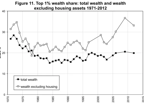
Understanding the dynamics of wealth concentration: the role of housing
In the discussion of average wealth, we identified the role of housing wealth, and this has been the concern of a number of commentators on the rise of capital described by Piketty (2014) – see, for example, Bonnet et al (2014), Turner (2014) and Rognlie (2015). The earlier time series analysis by Atkinson, Gordon and Harrison (1989) had identified one of the key determinants of the dynamics of UK top wealth shares up to the end of the 1970s as “popular wealth”, the sum of owner-occupied housing plus consumer durables. In particular, the authors stressed the role of house prices as reducing the share of the top 1 per cent. Since then, there have been major changes in the UK housing market. The role of housing wealth has to be seen in terms of the tenure changes. The popular wealth variable (leaving aside consumer durables) depended on both house prices and the extent of owner-occupation. It is changes in the latter that drove much of the variation between 1920s and 1970s: the proportion of owner-occupied in England and Wales rose from 23 per cent of households in 1918 to 50 per cent in 1971, and to 58 per cent in 1981 (all of the figures in this paragraph come from Office for National Statistics, 2013, unless otherwise indicated). This coincided with the fall in housing owned by private landlords: from 76 per cent in 1918, to 11 per cent in 1981. Both factors led to a decline in the share of the top 1 per cent, which contained a disproportionate number of landlords. The shift from private-rented to owner-occupied did not in itself change the ratio of housing wealth to the total personal wealth (different people owned the same houses),