Turbulent Von Kármán flow between two counter-rotating disks

HAL Id: hal-00170265

https://hal.archives-ouvertes.fr/hal-00170265

Submitted on 7 Sep 2007

HAL is a multi-disciplinary open access

archive for the deposit and dissemination of

sci-entific research documents, whether they are

pub-lished or not. The documents may come from

teaching and research institutions in France or

abroad, or from public or private research centers.

L’archive ouverte pluridisciplinaire HAL, est

destinée au dépôt et à la diffusion de documents

scientifiques de niveau recherche, publiés ou non,

émanant des établissements d’enseignement et de

recherche français ou étrangers, des laboratoires

publics ou privés.

Turbulent Von Kármán flow between two

counter-rotating disks

Sébastien Poncet, Roland Schiestel, Romain Monchaux

To cite this version:

Sébastien Poncet, Roland Schiestel, Romain Monchaux. Turbulent Von Kármán flow between two

counter-rotating disks. 8th ISAIF, Jul 2007, Lyon, France. pp.141-150. �hal-00170265�

Proceedings of the 8th _{International Symposium} on Experimental and Computational

Aerothermodynamics of Internal Flows Lyon, July 2007

Sébastien PONCET: Associate Professor

http://www.l3m.univ-mrs.fr/

Paper reference: ISAIF8-0013

Turbulent Von Kármán flow between two counter-rotating disks

Sébastien Poncet*, Roland Schiestel†, Romain Monchaux‡

*MSNM-GP, UMR 6181, Technopôle Château-Gombert, 38 rue F. Joliot-Curie, 13451 Marseille – France †IRPHE, UMR 6594, Technopôle Château-Gombert, 49 rue F. Joliot-Curie, BP 146, 13384 Marseille – France ‡ DSM/DRECAM/SPEC/GIT, URA 2464, CEA Saclay, 91191 Gif sur Yvette - France

The present work considers the turbulent Von Kármán flow generated by two coaxial counter-rotating smooth (viscous stirring) or bladed (inertial stirring) disks enclosed by a cylindrical vessel. Numerical predictions based on one-point statistical modeling using a low Reynolds number second-order full stress transport closure (RSM) are compared to velocity measurements performed at CEA. An efficient way to model the rule of straight blades is proposed. The influences of the rotational Reynolds number, the aspect ratio of the cavity, the rotating disk speed ratio and of the presence or not of impellers are investigated to get a precise knowledge of the dynamics and the turbulence properties in the Von Kármán configuration. In particular, we highlighted the transition be-tween the Batchelor [1] and the Stewartson [25] flow structures and the one bebe-tween the merged and separated boundary layer regimes in the smooth disk case. We determined also the transition between the one cell and the two cell regimes for both viscous and inertial stirrings.

Keywords: Von Kármán flow, counter-rotating disks, turbulence modeling, Reynolds Stress Model

Introduction

The flow between two finite counter-rotating disks enclosed by a cylinder, known as the Von Kármán [27] geometry, is of practical importance in many industrial devices. Counter-rotating turbines may indeed be used to drive the counter-rotating fans in gas-turbine aeroengines. Moreover, this configuration is often used for studying fundamental aspects of developed turbulence and espe-cially of magneto-hydrodynamic turbulence.

From an academic point of view, the laminar flow between two infinite disks has indeed justified many works since the beginning of the controversy between Batchelor [1] and Stewartson [25] on the flow structure. Batchelor [1] solved the system of differential equations

relative to the steady rotationally-symmetric viscous flow between two infinite disks. In the exactly counter-rotating regime, the distribution of tangential velocity is symmetrical about the mid-plane and exhibits five zones: one boundary layer on each disk, a transition shear layer at mid-plane and two rotating cores on either side of the transition layer. As stated by Batchelor him-self, ``this singular solution may not be realizable ex-perimentally, of course''. In 1953, Stewartson [25] found that the flow is divided into three zones for large values of the Reynolds number based on the interdisk spacing H:

100 /ν

ΩH

Re_H = 2 > (Ω the rotation rate of the disks and ν the kinematic viscosity of the fluid): one boundary layer on each disk separated by a zone of zero tangential velocity and uniform radial inflow. Kreiss and Parter [15]

have proved the existence and non-uniqueness of solu-tions at sufficiently large Reynolds numbers for the two-disk configuration. Thus, both Batchelor and Stew-artson solutions are possible depending on the initial and boundary conditions but the Batchelor prediction has not been mentioned in the literature for the exact counter-rotating disk case. The reader is referred to the work of Holodniok et al. [13] and to the review of Zandbergen and Dijkstra [28] for a more extensive sur-vey until 1987.

In the turbulent case, the Von Kármán flow is a model flow to study the turbulence characteristics on small scales. The main flow is axisymmetric and so offers an interesting intermediate situation between two-dimensional and three-dimensional flows. Maurer et al. [17] established, using low-temperature helium gas, the turbulence characteristics (structure functions, PDF of the velocity differences) and confirmed that turbulence on small scales has universal properties independent of the forcing. Mordant et al. [19] investigated the dynami-cal behavior of the Von Kármán flow at moderate to high Reynolds numbers using spatially averaged measure-ments. Data of the power input and of pressure fluctua-tions at the wall are sufficient to calculate the main tur-bulence characteristics. Cadot and Le Maître [6] consid-ered the turbulent flow between two counter-rotating stirrers. They measured the instantaneous torques driving the flow and compared them to similarity laws having no dependence on the Reynolds number with a good agree-ment. Ravelet et al. [22,24] reported experimental evi-dence of a global bifurcation on a highly turbulent flow between two counter-rotating impellers. The transition between the symmetric and the unsymmetric solutions is subcritical and the system keeps a memory of its history. Monchaux et al. [18] investigated the properties of the mean and most probable velocity fields in the same con-figuration. They showed that these two fields are de-scribed by two families of functions depending on both the viscosity and the forcing. For large values of the Reynolds number, a tendency for Beltramization of the flow is obtained. Boronski [3] simulated the laminar Von Kármán flow between two counter-rotating disks equipped or not by straight blades. For a rotational Rey-nolds number based on the disk radius R, equal to 500, the poloidal-to-toroidal ratio is increased from 13% in the smooth disk case to 51% in the bladed disk case.

A renewal of interest for the Von Kármán flow is born from the dynamo experiments. The flow between counter-rotating impellers is indeed considered as a pos-sible candidate for the observation of a homogeneous fluid dynamo less constrained than the Riga and Karlsruhe devices. The flow needs to be highly turbulent in order for nonlinearities to develop in the magnetic

induction. Numerous experimental [26] or numerical [4,23] studies have then been dedicated to mag-neto-hydrodynamics turbulence in the Von Kármán ge-ometry.

To our knowledge, only very few numerical works have been devoted to the characterization of the mean and turbulent flow properties in the Von Kármán geome-try. Kilic et al. [14] performed a combined numerical and experimental study of the transitional flow between smooth counter-rotating disks for-1≤Γ≤0, Re=105 and G=H/R=0.12, where Γ is the ratio between the rotat-ing speeds of the two disks and G is the aspect ratio of the cavity. They compared mean radial and tangential velocity measurements using a single-component laser Doppler anemometer with computed results either a clas-sical low-Reynolds number k-ε turbulence model or a laminar elliptic code. ForΓ=-1, the weakly turbulent flow is of Stewartson type, whereas the laminar compu-tations and measurements produce a Batchelor type of flow. The transitions from laminar to turbulent regime and from Batchelor to Stewartson flow structure occur forΓ=−0.4. A good agreement is obtained in the ro-tor-stator configuration ( Γ=0) and in the exactly counter-rotating regime (Γ=-1) but at intermediate val-ues of Γ, the agreement is less satisfactory.

In this paper, we present comparisons between nu-merical predictions using a Reynolds Stress Model, de-noted RSM, and velocity measurements performed at CEA for the turbulent flow between two counter-rotating disks. The main objective is to acquire a precise knowl-edge of both the flow structure and the turbulence prop-erties of the high turbulent Von Kármán flow between smooth disks for a large range of the flow control pa-rameters. A second objective is to propose an easy and efficient way to model impellers and to quantify their effect on the Von Kármán flow at high Reynolds number.

Experimental Procedure

Geometrical model

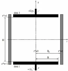
We consider the Von Kármán flow generated by two counter-rotating disks enclosed by a cylindrical vessel, as illustrated in Fig. 1. The cylinder radius and height are respectively, Rc=100 mm and Hc=500 mm. The radius ratio R/Rc between the rotating disk radius R and the cylinder radius is fixed to 0.925. The distance between the inner faces of the disks H can vary between 10 and 180 mm. We use bladed disks to ensure inertial stirring or flat disks for viscous stirring. The impellers are driven by two independent 1.8 kW motors, with speed servo loop control. The motor rotation rates Ω₁ and Ω₂ can be varied independently in the range 0-900 rpm,

Sébastien PONCET et al. Turbulent Von Kármán flow between two counter-rotating disks 3

withΩ₁ ≥ Ω₂ . The working fluid is water.

Fig. 1 Sketch of the cavity and relevant notation.

Flow control parameters

The main flow is controlled by the ratio between the two rotation ratesΓ=−Ω₂/Ω₁, the aspect ratio of the cavity G=H/Rc and the rotational Reynolds num-berRe=Ω₁R2_c/ν. In the case of inertial stirring, the number of straight blades n and their dimensionless height h*=h/Rc are also considered.

Measurement technique

Velocity measurements are done using a laser Doppler velocimetry (LDV). A basic measurement is a two min-utes acquisition of 190000 randomly sampled values of one velocity component at one point of the flow. Due to geometry reasons, we have access to the axial V_zand tangential V_θmean velocity components. From this raw data, one may compute the time-averaged flow point by point on a 11*15 grid.

Statistical modeling

The predictions of the Reynolds Stress Model (RSM) used in the present work have already been validated in the rotor-stator configuration (Γ=0) [10,21] for a wide range of aspect ratio G and Reynolds number Re. It showed that this level of closure is adequate in such flow configurations, while the usual k-ε model, which is blind to any rotation effect presents serious deficiencies. Thus, the purpose of this paper relying on a well established turbulent model is to extend its application to new flow conditions and to get a better insight into the dynamics of the highly turbulent Von Kármán flow. The reader is thus referred to [9,10,20,21] for more details about the model and the numerical method.

The differential Reynolds Stress Model (RSM) The flow studied here presents several complexities (high rotation rate, wall effects, transitional zone, shear layer), which are severe demands for turbulence model-ing methods. Our approach is based on one-point statis-tical modeling using a low Reynolds number sec-ond-order full stress transport closure derived from the Launder and Tselepidakis [16] model and sensitized to rotation effects [10]. This approach allows for a detailed description of near-wall turbulence and is free from any eddy viscosity hypothesis. The general equation for the Reynolds stress tensor R_ijcan be written:

ij P_ij D_ij Φ_ij ε_ij T_ij dt dR + − + + = (1) where P_ij, D_ij, Φ_ij, ε_ijand T_ijrespectively denote the production, diffusion, pressure-strain correlation, dissipation and extra terms. The diffusion termD_ijis split into two parts: a turbulent diffusion D , which is in-T_ij terpreted as the diffusion due to both velocity and pres-sure fluctuations and a viscous diffusion D_ijν, which cannot be neglected in the low Reynolds number region. In a classical way, the pressure-strain correlation term

ij

Φ can be decomposed as below: (1) (2) (w) ij Φ ij Φ ij Φ ij Φ = + + (2) (1) ij

Φ is interpreted as a slow nonlinear return to isotropy and is modeled as a quadratic development in the stress anisotropy tensor, with coefficients sensitized to the in-variants of anisotropy. This term is damped near the wall. The linear rapid part (2)

ij

Φ includes cubic terms. A wall correction (w)

ij

Φ is applied to the linear part which is modeled using the Gibson and Launder hypothesis [12] with a strongly reduced numerical coefficient. However the widely adopted length scale k3/2/εis replaced by the length scale of the fluctuations normal to the wall. The viscous dissipation tensor has been modeled in order to conform with the wall limits obtained from Taylor series expansions of the fluctuating velocities. The extra term

ij

T accounts for implicit effects of the rotation on the turbulence field. It contains additional contributions in the pressure-strain correlation, a spectral jamming term, inhomogeneous effects and inverse flux due to rotation, which impedes the energy cascade [7].

The dissipation rate ε equation to solve is the one proposed by Launder and Tselepidakis [16]. The turbu-lence kinetic energy k equation which is redundant in a

RSM model is still solved, in order to get faster numeri-cal convergence. It is verified that after convergence the turbulence kinetic energy is exactly equal toR_jj/2.

Numerical method

The computational procedure is based on a finite volume method using staggered grids for mean velocity components with axisymmetry hypothesis in the mean. The computer code is steady elliptic and the numerical solution proceeds iteratively. We have verified that a 120² mesh in the (r,z) frame is sufficient in smooth rotating disk cases to get grid-independent solutions. A refined mesh 160² is necessary to model flows with straight blades. It is to be compared to the 140 x 80 mesh used by Elena and Schiestel [9,10] and Poncet et al. [20,21] in rotor-stator systems. The calculation is initialized using realistic data fields, which satisfy the boundary condi-tions. About 20000 iterations (several hours on the bi-Opteron 18 nodes cluster of IRPHE) are necessary to obtain the numerical convergence of the calculation. The stress component equations are solved using matrix block tridiagonal solution to enhance stability using non stag-gered grids.

Boundary conditions

At the wall, all the variables are set to zero except for the tangential velocityV_θ, which is set to Ω₁r on disk 1, -Ω₂ron disk 2 and zero on the cylinder. At the pe-riphery of the disks (R≤r≤R_c) V_θis supposed to vary linearly from zero on the cylinder up to Ω₁Ron disk 1 and -Ω₂R on disk 2 and the radialV_rand axialV_z ve-locity components are fixed to zero.

We can not implement real straight blades in our two-dimensional code. So we limit to modeling their most important effect, which is to increase the efficiency of the disks in forcing the flow. Thus, we add a volumic drag force f in the equation of the tangential velocity componentV_θ. If we consider n straight blades, the volumic drag force f can be written as:

C_DV_relV_rel r ρ 4π n r F 2π n f = = (3) where F is the drag force of one blade, ρ the fluid density,

D

C the dimensionless drag coefficient and

θ

i rel Ω r V

V = − the relative tangential velocity on disk i=1,2. The force is designed to make the fluid velocity closer to the local disk velocity near the disks. This form is close to the one proposed by Boronski [3] for spectral code. For curved blades, the same approach can be used: a volumic lift force can be added in the equation of the radial velocityV . It will be the subject of a next study. _r

Some calculations have been performed forΓ=-1,

G=1.8, Re=2.105and straight blades (h*=0.2, n=8) to study the influence of the trailing coefficientC . The _D differences on the extrema of the tangential velocity component are inferior to 0.5% forC_D in the range [0.1-2]. Thus, we have chosen to fix the value of C _D equal to 0.5, which agrees with the values proposed by Blevins [2] in the case of a thin rectangular plate perpen-dicular to an uniform flow.

Smooth disk case: viscous stirring

In this section, we consider the turbulent flow between two counter-rotating flat smooth disks. Thus, we ensure a viscous stirring and we investigate the influence of the Reynolds number Re, the aspect ratio of the system G, and the ratio Γ between the two rotation rates on the mean and turbulent fields.

Flow structure in the exact counter-rotating regime

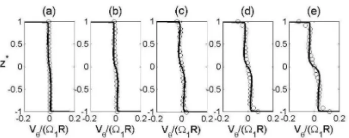
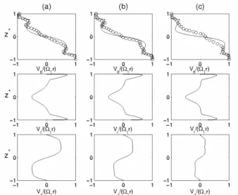
Fig. 2 Axial profiles of the tangential velocity for Γ=-1,

5

10 6.28 =

Re × and G=1.8 at (a) r*=0.35, (b) r*=0.48, (c) r*=0.61, (d) r*=0.74, (e) r*=0.87. Comparisons between the numerical results (lines) and the experimental data (symbols) in the smooth disk case.

The structure of the mean flow in the exact counter-rotating regime is henceforth globally well known: it can be decomposed into two toroidal cells in the tangential direction (not modelled here because of the axisymmetry hypothesis) and into two poloidal recircula-tions in the (r,z) plane. We focus here on the poloidal cells (Fig.6a): the fluid at the top and the bottom of the cavity is forced into two opposite rotation speeds, and is then entrained by the disks. Consequently, a shear layer develops in the equatorial plane. This is perceptible in Fig.2, which presents axial variations of the tangential velocity component forΓ=-1,Re=6.28×105, G=1.8 at five radial locations in the range r*=0.35-0.87. The radial and axial velocity components are not presented here because they are almost zero in the whole cavity both in the experiments and in the calculations. The tangential component is quite weak too except in the two very thin boundary layers, which develop on each disk and whose size is shown in Fig.3 and close to the periphery, where the shear layer is observed.

Sébastien PONCET et al. Turbulent Von Kármán flow between two counter-rotating disks 5

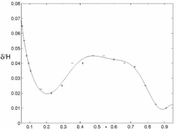
Fig. 3 Radial distribution of the boundary layer thickness δ/H

(symbols: RSM, lines: polynomial interpolation). See legend Fig.2.

For r* < 0.48 (Fig.2a), the profile exhibits a Stewartson flow structure: a quasi zero tangential velocity zone en-closed by two boundary layers on each disk. The flow in the boundary layers is characterized by a strong tangen-tial velocity component (positive on disk 1 and negative on disk 2) and by a radial outward component not shown here. Towards the periphery (Fig.2b-e), the flow gets of Batchelor type with five distinct zones: two boundary layers on the disks, a shear layer at mid-plane and two zones enclosed between the two. These last two zones are characterized by a weak but non zero tangential velocity component. The shear layer thickens when the local ra-dius r* increases. Contrary to the laminar case reported by Kilic et al. [14], there is practically no radial inflow around z*=0. A good agreement between the numerical results and the experimental data is obtained even the values are quite weak. The RSM model catches the ap-pearance and the thickening of the shear layer. The agreement between the numerical predictions and the measurements is less satisfactory in the boundary layers as it can be seen Fig.2. These zones are in fact hardly attainable by LDV measurements.

The transition between the Stewartson and Batchelor flow structures can also be seen in Fig.3 from the radial evolution of the boundary layer thickness δ for the same set of parameters. Very close to the rotation axis, the ax-ial flow impinges the disks and creates very large bound-ary layers on both disks, whose size decreases with the local radius. The flow is then of Stewartson type. During the transition, δ increases as already observed by Poncet [20] for rotor-stator flows (Γ=0). Forr*≈ 0.47, the flow is clearly of Batchelor type and then, δ decreases towards the periphery of the cavity.

We investigate the influence of the Reynolds number on the mean flow. Fig.4 presents radial profiles of the tangential velocity component forΓ=-1, G=1.8 and four Reynolds numbers at different axial locations. The

nu-merical predictions of the RSM model are compared to present LDV measurements and to the velocity meas-urements of Ravelet [22] forRe≥ 105. These data are also compared to the local disk 1 and disk 2 velocities.

Fig. 4 Radial profiles of the tangential velocity for Γ=-1 and

G=1.8 at (a) z*=0.91, (b) z*=0.59, (c) z*=0.02, (d) z*=-0.59, (e) z*=-0.92.

The numerical data for Re≥≥≥≥ 6.28×105 merge al-most into a single fitting curve. It means that there is practically no effect of the Reynolds number on the mean field ever since the flow is turbulent. For Re=2×105, a significant increase of the magnitude of V is observed _θ whatever the axial position, which is characteristic of the laminar regime. The critical Reynolds number for the transition from the laminar to the turbulent state is thus overestimated compared to the one obtained by Ravelet [22]:Re=105. Nevertheless, the present velocity meas-urements performed on the same experimental set-up as [22] confirm the numerical results. Compared to the pre-vious measurements, an effect of Re is observed on the radial profiles of V at the periphery of the cavity. In _θ fact, the critical Reynolds number for the laminar to tur-bulent state transition depends strongly on the boundary conditions and especially on the conditions imposed in the radial gap. We recall that a linear profile is imposed in the numerical code forV , that does not take into ac-_θ count any recirculation zone and that could explain this difference. This tendency for relaminarization of the RSM model has already been noticed by Poncet et al. [20,21] in the rotor-stator configuration. As a conclusion, there is no significant effect of the Reynolds number on the mean flow forRe≥ 105, which confirms the results of Cadot et al. [5] and Ravelet [22].

Fig.6a presents the corresponding streamline patterns. The mean flow is divided into two symmetric poloidal cells, whose size is equal here to 0.5 H along the axial

direction and independent of the Reynolds number. In the radial direction, the diameter of the largest eddies ob-served is of the order of the disk radius R, showing this scale is the order of the energy scale injection.

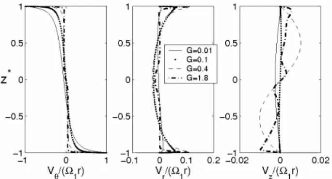
Fig. 5 Axial profiles of the mean velocity components for

r*=0.81, Γ=-1,Re=1.3×106 and viscous stirring (RSM).

The influence of the aspect ratio of the cavity G on the mean field has also been investigated for G=[0.01;1.8]

(Fig.5) and a given Reynolds numberRe=1.3×106. For G=1.8, the boundary layers are separated as already men-tioned and the mean tangential velocity component is constant in the core of the flow. When one decreases the aspect ratio, the flow gets of torsional Couette type with merged boundary layers. For G=0.01, V (Fig.5a) var-_θ ies indeed linearly in the median region of the flow. The transition between the merged and the separated bound-ary layer regime occurs for G=0.4. This is to be com-pared to the value G=0.012 obtained in the rotor-stator configuration [21]. The transition is continuous and not clear from the V -profile. Nevertheless, if we consider _θ the V_z-profile (Fig.5c), we can clearly see that the axial velocity component is almost zero whatever the value of G, expect for G=0.4, where the fluid moves towards the upper and lower disks. The transition can also be charac-terized by considering the V_r-profiles (Fig.5b), which exhibit the thinning of the boundary layers for increasing values of the aspect ratio.

Flow structure for -1≤≤≤≤ _Γ≤≤≤≤0

Another interesting feature in counter-rotating disk flows is the influence of the ratio Γ between the two ro-tating disk speeds (Fig.6). The Reynolds number and the aspect ratio of the cavity are respectively fixed to Re=1.3×106 and G=1.8. We focus on the counter-rotating disk case for which Γ= [-1; 0]. In the exact counter-rotating regime (Fig.6a), the flow is sym-metric and two cells with the same size 0.5 H coexist. For small rotating speed differences, the structure of the

mean flow is strongly dominated by the faster disk (Fig.6b-e). Varying the ratio Γ displaces the shear layer towards the slower disk. The cell close to the lower disk invades almost the whole interdisk spacing for Γ=-0.7 (Fig.6d). For Γ=-0.2 (Fig.6e), the flow structure resem-bles the one observed in the rotor-stator configuration [20] with streamline patterns parallel to the rotating axis.

Fig. 6 Computed streamlines patterns between smooth disks for

G=1.8, Re=1.3×106 and (a) Γ=-1, (b) Γ=-0.9, (c) Γ=-0.8, (d)

Γ=-0.7, (e) Γ=-0.2.

This transition between the two cell and the one cell regimes can be seen also from Fig.7. It presents the evo-lution with Γ of the dimensionless size S_c/H of the smallest cell (along the upper disk) in the axial direction defined in Fig.6b. In the smooth disk case, we notice that

c

S decreases rapidly for decreasing values of |Γ| in the range [-1; -0.8] followingS_c/H∝-2.2Γ. For smallest values of |Γ|, the cell is reduced to a very thin region at-tached to the upper disk (Fig.6d-e), which disappears progressively along the external cylinder and so Sc

tends to zero.

Fig. 7 S_c/Hagainst Γ for G=1.8 (RSM). Comparisons

be-tween the (-) smooth disk case (Re=1.3×106), the (--) bladed disk case and previous results of (o) Kilic et al. [14] and (◊) Gan et al. [11].

In Fig.7, our results are compared to the ones obtained by Kilic et al. [14] and Gan et al. [11], who performed calculations for Γ= [-1; 0] and G=0.12 using a classical

Sébastien PONCET et al. Turbulent Von Kármán flow between two counter-rotating disks 7

k-ε turbulence model. ForRe =105, Kilic et al. [14] found that the evolution of S_cagainst Γ is non monotonous. It decreases more slowly from Γ=-1 to Γ=-0.2 than in our case. It is a combined effect of both the Reynolds number and the aspect ratio of the cavity. For Γ=-0.4, they ob-served a double transition: from laminar to turbulent flow and from Batchelor to Stewartson type of flow. The de-crease of S_cis much faster with Γ in the laminar case

[14]. ForRe=1.25×106, Gan et al. [11] obtained stream-line patterns different from the ones shown in Fig.6 for Γ =[-0.8;-0.2] essentially because of the small value of G. A large cell along the slower disk is still observed for

Γ=-0.4. This cell is trapped by the main flow due to the

faster disk in the zone r*=0.3-0.45.

Turbulence field in the exact counter-rotating regime

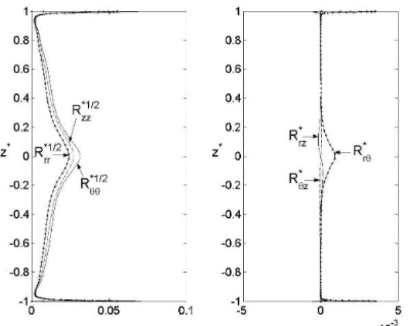
Fig. 8 Axial profiles of the Reynolds stress tensor at r*=0.81 for

Γ=-1, G=1.8 and Re=6.28×105 in the smooth disk case

(RSM).

As already mentioned below, there is practically no effect of both the Reynolds number and the aspect ratio on the mean flow. In the following, we focus on the exact counter-rotating regime Γ=-1 and Re and G are fixed respectively to Re=6.28×105 and G=1.8. Fig.8 pre-sents the axial profiles of the six components of the Reynolds stress tensor. These components are normalized by the local disk 1 velocity. For example, R*_rr is de-fined as:R*_rr =v'2_r/(Ω₁r)2. As in all rotating disk prob-lems [21], turbulence is mainly concentrated in the boundary layers with the same turbulence levels in the upper and lower disk boundary layers. The main differ-ence with the rotor-stator configuration is that turbuldiffer-ence is also generated in the median region of the interdisk spacing and is due to the shear, stretched by the recircu-lations. The Von Kármán arrangement is indeed known to

produce an intense turbulence in a compact region of space [17]. The magnitudes of the three normal compo-nents (in principal axes) are almost the same in the equa-torial plane. It means that turbulence is quasi isotropic in that region. The cross components are quite weak except for the R*_rθ component, which behaves like the normal components with a bump at mid-plane.

Bladed disk case: inertial stirring

To increase the efficiency of the disks in forcing the flow, we used n blades of height h* mounted on both disks. The stirring is called inertial because the fluid is set into motion thanks to areas of forcing perpendicular to the motion itself. In that case, Ravelet [22] showed that all mean and turbulent quantities are independent of the Reynolds number in the rangeRe=[105,2×106]. Thus, we have chosen to fix the values of Re=2×105 and G=1.8. In that case, the boundary layers are sepa-rated and the flow is found to be highly turbulent. More-over, direct comparisons with the experiments of Ravelet [22] can be performed. The purpose of this section is to propose an efficient way to model the effect of straight blades on both the mean and turbulent fields.

Flow structure in the exact counter-rotating regime In the bladed disk case, the flow structure is com-pletely different from the smooth disk case, where the velocity gradient are located in the boundary layers along the disks and decrease when the Reynolds number in-creases. For an inertially driven flow, the mean flow does not present any appreciable velocity gradient in the vi-cinity of the blades (Fig.9) and the gradients are distrib-uted in the median region of the flow. The mean flow is divided into three main regions: a shear layer at mid-plane and two fluid regions close to each bladed disk. The intensity of the shear at mid-plane is increased com-pared to the viscous stirring case. This shear is due to the two recirculation cells. It induces a strong radial inflow (V <0) around z*=0 and two opposite axial flows to-_r wards the disks. The magnitude of the mean axial and radial velocity components increase from the periphery (Fig.9c) to the rotation axis (Fig.9a). From the disk to the top of the blades, the tangential fluid velocity is fairly close to the local disk velocity. Moreover, a strong radial outflow is created along the bladed disks and goes with the impellers. At the top of the blades, there is a strong decrease of |V | interpreted as the wake of the blades. _θ

There is a very good agreement between the numerical predictions and the velocity measurements concerning the V -profiles. A small difference is observed in the _θ shear layer, where the RSM model predicts a thinner

layer than the one measured by Ravelet [22]. This last author observed, for the same set of parameters, high energy levels for frequencies inferior to the injection fre-quency. This contribution is attributed to the appearance of strong coherent structures in the shear layer not ob-served in the smooth disk case and which may explain the weak discrepancies obtained.

Fig. 9 Axial profiles of the mean velocity components for Γ=-1,

G=1.8 and Re=2×105 and bladed disks (n=8, h*=0.2) at (a) r*=0.4, (b) r*=0.5, (c) r*=0.6. Comparisons between the nu-merical predictions (lines) and the LDV data of Ravelet [22] (symbols).

Flow structure for -1≤≤≤≤ _Γ≤≤≤≤0

Fig. 10 Computed streamlines patterns between bladed disks

(n=8, h*=0.2) for G=1.8, Re=2×105 and (a) Γ=-1, (b)

Γ=-0.9, (c) Γ=-0.8, (d) Γ=-0.7, (e) Γ=-0.6.

We perform the same analysis as in the smooth disk case by varying the ratio Γ between the two rotating disk speeds. Fig.10presents comparisons between the smooth and bladed disk cases concerning the size Scof the cell

along the slowest disk for Γ = [-1; 0]. The same behavior is obtained but the transition between the two cell and the one cell structures (S_c→→ ) is slightly delayed. It occurs →→0 in the inertial stirring case for Γ =-0.65, which is close to the experimental value obtained by Cadot and Le Maître [6] in the same configuration Γ=-0.69 and the analytical

one obtained by Dijkstra and Van Heijst [8] for 0

→

e

R in the smooth disk case Γ =-2/3. The measure-ments of Ravelet [22] reveal a transition for Γ =-0.78. It confirms the similitude observed by [6] between the smooth disk flow with a large viscosity and the mean flow in the inertial stirring case.

The transition from the two cell to the one cell struc-tures can be seen also from Fig.7 Compared to the smooth disk case, the cell along the slowest disk is larger for Γ=-0.8 (Fig.10c). For Γ=-0.7, only a small recircula-tion subsists along the upper disk and completely disap-pears for Γ=-0.6. ForΓ≥≥≥≥-0.6, the same pattern is ob-served with streamlines parallel to the rotation axis.

Turbulence field in the exact counter-rotating regime

Fig. 11 Axial profiles of the Reynolds stress tensor at r*=0.81

for Γ=-1, G=1.8 and Re=2×105 and bladed disks (n=8, h*=0.2). (lines) RSM and (o) LDV data [22].

To enable direct comparisons with the viscous stirring case, Fig.11 presents the axial profiles of the six compo-nents of the Reynolds stress tensor at the same radius r*=0.81 and for the same values of G and Γ. The main difference between the smooth and the bladed disk con-figurations is that, in the latter case, the turbulence inten-sities vanish towards the disks. Apart from that, turbu-lence is also mostly generated at mid-plane because of the shear stretched by the recirculations. The blades in-duce a much stronger shear zone in the equatorial plane compared to the smooth disk case as already seen from the mean velocity profiles (Fig.9). Thus, the turbulence levels, regarding the normal Reynolds stress components (Fig.11), are almost 20 times larger than for viscous stir-ring and quite comparable to the mean fluid velocity. It confirms the previous measurements of Cadot et al. [5] in steady regimes of turbulence in the Von Kármán geome-try. They found that the fluid velocity fluctuations are close to the fluid mean velocity and 6 times larger in the

Sébastien PONCET et al. Turbulent Von Kármán flow between two counter-rotating disks 9

bladed disk case than in the smooth disk case. In the pre-sent study, the R*_rrcomponent is much weaker than the two other normal components, which indicates the tur-bulence anisotropy in the core of the flow. The cross components are also stronger than in the smooth disk case. The level of the R*_rθcomponent (Fig.11) is of the order ofR*_rr. Note that the maximum of the R*_θθ com-ponent obtained at mid-plane (z*=0) using the RSM model is in excellent agreement with the asymptotic value measured by Ravelet [22] for Re larger than 10000 (relative error inferior to 0.1%).

Fig. 12 Radial profiles of the turbulence kinetic energy k* at

z*=0 for Γ=-1, G=1.8 and Re=2×105(RSM).

To study the influence of the number n of blades and their height h* on the turbulent field, Fig.12 shows radial profiles of the turbulence kinetic energy k* normalized by (Ω₁R_c)2 for various impeller configurations. These profiles are plotted at mid-plane where the maximum of k* prevails. As expected, k* increases towards the pe-riphery of the cavity, it means for increasing local Rey-nolds number. Then, k* decreases for radial locations in the gap between the disks and the external cylinder. We can first notice the very weak level of turbulence kinetic energy in the smooth disk case compared to the bladed disk cases. Secondly, the influence of the blade number n is quite weak for n=4, 8 or 16. Only very close to the rotation axis, we can notice a different behavior in the configuration with 16 blades. Nevertheless, in the whole flow, four blades seem to be sufficient to force the flow. On the other hand, the blade height h* plays a more im-portant role. The k* level is twice higher when the blades are twice higher too. Ravelet [22] showed that all mean and turbulent quantities are independent of the Reynolds number in the rangeRe=[105,2×106]. The turbulent dissipation is indeed much stronger than the dissipation

due to the boundary layers and hides the dependence on Re. All these results can thus be extended to higher Rey-nolds numbers.

Conclusion

We have performed some comparisons between nu-merical predictions using a RSM model and velocity measurements considering the turbulent flow between two flat or bladed counter-rotating disks. This configura-tion known as the Von Kármán geometry is used to pro-duce an intense turbulence in a compact region of space.

For viscous stirring, the flow is of Stewartson type close to the rotation axis and so exhibits three distinct regions: two boundary layers and one shear layer at mid-plane. When one approaches the periphery of the cavity, forr*≈0.48, the flow gets of Batchelor type. Turbulence is mainly concentrated in the boundary layers and in the transitional shear layer, where turbulence is almost isotropic. Turbulence intensities increase towards the outer cylinder. While the aspect ratio of the cavity G is lower than 0.4, the boundary layers are mixed and the flow is then of torsional Couette type. In the case of iner-tial stirring, the impellers are more efficient to force the flow. Thus, the transitional shear layer intensifies. Tur-bulence is so mainly concentrated around z*=0 and van-ish towards the disks. The turbulence intensities are al-most 20 times larger than in the flat disk case. The height of the blades is found to be the preponderant parameter to increase the turbulence intensities more than the number of blades. In the flat and bladed disk cases, we have nu-merically verified the statement of Cadot et al. [5]: ``smooth or rough, the efficiency of a given type of stir-rer to set the bulk of the fluid in motion is independent of the Reynolds number''. Moreover, we have characterized the transition between the two cell and the one cell re-gimes. For inertial stirring, it occurs for Γ≈−0.65close to the values obtained by [6,8].

The agreement between the numerical predictions and the LDV measurements is very satisfactory in both cases. For the first time, an easy and efficient way to model the main effect of straight blades has been proposed. Further experimental works are now required to provide more comparisons for the turbulent fields but also some calcu-lations for curved blades.

References

[1] Batchelor, G. K.: Note on a class of solutions of the Na-vier-Stokes equations representing steady rotation-ally-symmetric flow, Quat. J. Mech. Appl. Math., vol.4, pp.29-41, (1951).

[2] Blevins, R.D.: Applied fluid dynamics handbook, Ed. Van Nostrand Reinhold Company Inc., New-York, (1984).

[3] Boronski, P.: Méthode des potentiels poloïdal-toroïdal ap-pliquée à l'écoulement de Von Kármán en cylindre fini, PhD Thesis, Ecole Polytechnique, Palaiseau, (2005).

[4] Bourgoin, M., et al.: An iterative study of time independent induction effects in magnetohydrodynamics, Phys. Fluids, vol.16, pp. 2529-2547, (2004).

[5] Cadot, O. et al.: Energy injection in closed turbulent flows: stirring through boundary layers versus inertial stirring, Phys. Rev. E, vol.56, pp.427-433, (1997).

[6] Cadot, O., Le Maître, O.: The turbulent flow between two rotating stirrers: similarity laws and transitions for the driving torques fluctuations, Eur. J. Mech. B/Fluids, in press, pp.427-433, (2006).

[7] Cambon, C., Jacquin, L.: Spectral approach to non-isotropic turbulence subjected to rotation, J. Fluid Mech., vol.202, pp.295-317, (1989).

[8] Dijkstra, D., Van Heijst, G.J.F.: The flow between two finite rotating disks enclosed by a cylinder, J. Fluid. Mech., vol.128, pp.123-154, (1983).

[9] Elena, L.: Modélisation de la turbulence inhomogène en présence de rotation, PhD thesis, Univ. Aix-Marseille II, (1994). [10] Elena, L., Schiestel, R.: Turbulence modeling of rotating confined flows, Int. J. Heat Fluid Flow, vol.17, pp.283-289, (1996).

[11] Gan, X., Kilic, M., Owen, J.M.: Superposed flow between two discs contrarotating at differential speeds, Int. J. Heat Fluid Flow, vol.15, pp.438-446, (1994).

[12] Gibson, M., Launder, B.E.: Ground Effects on Pressure Fluctuations in the Atmospheric Boundary Layer, J. Fluid. Mech., vol.86, pp.491-511, (1978).

[13] Holodniok, M., Kubicek, M., Hlavacek, V.: Computation of the flow between two rotating coaxial disks: multiplicity of steady-state solutions, J. Fluid. Mech., vol.108, pp.227-240, (1981).

[14] Kilic, M., Gan, X., Owen, J.M.: Transitional flow between contra-rotating disks, J. Fluid Mech., vol. 281, pp.119-135, (1994).

[15] Kreiss, H.O., Parter, S.V.: On the swirling flow between rotating coaxial disks: existence and uniqueness, Commun.

Pure Appl.Math., vol.36, pp.55-84, (1983).

[16] Launder, B.E., Tselepidakis, D.P.: Application of a new second-moment closure to turbulent channel flow rotating in orthogonal mode, Int. J. Heat Fluid Flow, vol.15, pp.2-10, (1994).

[17] Maurer, J., Tabeling, P., Zocchi, G.: Statistics of turbulence between two counterrotating disks in low-temperature helium gas, Europhys. Lett., vol.26, pp.31-36, (1994).

[18] Monchaux, R. et al.: Properties of steady states in turbulent axisymmetric flows, Phys. Rev. Lett., vol.96, 124502, (2006). [19] Mordant, N., Pinton, J.-F., Chilla, F.: Characterization of turbulence in a closed flow, J. Phys. II France, vol.7, pp.1729-1742, (1997).

[20]Poncet, S. : Ecoulements de type rotor-stator soumis à un flux axial: de Batchelor à Stewartson, PhD thesis, Université de Provence, (2005).

[21] Poncet, S., Chauve, M.P., Schiestel, R.: Batchelor versus Stewartson flow structures in a rotor-stator cavity with through-flow, Phys. Fluids, vol.17, (2005).

[22] Ravelet, F.: Bifurcations globales hydrodynamiques et magnétohydrodynamiques dans un écoulement de Von Kármán turbulent, PhD Thesis, Ecole Polytechnique, Palaiseau, (2005). [23]Ravelet, F., Chiffaudel, A., Daviaud, F., Léorat, J.: Toward an experimental Von Kármán dynamo: numerical studies for an optimized design, Phys. Fluids, vol.17, 117104, (2005). [24] Ravelet, F., Marié, L., Chiffaudel, A., Daviaud, F.: Multi-stability and memory effect in a highly turbulent flow: experi-mental evidence for a global bifurcation, Phys. Rev. Letters, vol.93, (2004).

[25] Stewartson, K.: On the flow between two rotating coaxial disks, Proc. Camb. Phil. Soc., vol.49, pp.333-341, (1953). [26] Volk, R., Odier, P., Pinton, J.-F.: Fluctuation of magnetic induction in Von Kármán swirling flows, Phys. Fluids, vol.18, 085105, (2006).

[27] Von Kármán, T.: Uber laminare und turbulente Reibung, Z. Angew. Math. Mech., vol.1, pp.233-252, (1921).

[28] Zandbergen, P.J., Dijkstra, D.: Von Kármán swirling flows, Ann. Rev. Fluid Mech., vol.19, pp.465-491, (1987).