Magnetization dynamics in magnetic nanostructures

HAL Id: tel-00006021

https://tel.archives-ouvertes.fr/tel-00006021v2

Submitted on 7 May 2004

HAL is a multi-disciplinary open access archive for the deposit and dissemination of sci-entific research documents, whether they are pub-lished or not. The documents may come from teaching and research institutions in France or abroad, or from public or private research centers.

L’archive ouverte pluridisciplinaire HAL, est destinée au dépôt et à la diffusion de documents scientifiques de niveau recherche, publiés ou non, émanant des établissements d’enseignement et de recherche français ou étrangers, des laboratoires publics ou privés.

Dana Elena Sorea Stanescu

To cite this version:

Dana Elena Sorea Stanescu. Magnetization dynamics in magnetic nanostructures. Condensed Matter [cond-mat]. Université Joseph-Fourier - Grenoble I, 2003. English. �tel-00006021v2�

présentée par

Dana Elena SOREA STANESCU

pour obtenir le titre de

D

OCTEUR DE L

’

UNIVERSITE

J

OSEPH

F

OURIER

–

G

RENOBLE

1

spécialité:

PHYSIQUE

____________________________________________

M

AGNETIZATION DYNAMICS

IN MAGNETIC NANOSTRUCTURES

_____________________________________________

Date de soutenance: 1 décembre 2003

COMPOSITION DU JURY

:

Theo RASING

Rapporteur

Claude CHAPPERT

Rapporteur / Président du jury

Jean-Louis PORTESEIL

Examinateur

Eric BEAUREPAIRE

Examinateur

Pascal XAVIER

Invité

Ursula EBELS

Invité

Kamel OUNADJELA

Directeur de thèse

Thèse préparée au sein des laboratoires :

REMERCIEMENTS

Ce travail de thèse a été réalisé dans le Département de Recherche Fondamentale sur la Matière Condensée (DRFMC) du CEA/Grenoble, dans le laboratoire SPINTEC.

Mes remerciements s’adressent tout d’abord aux membres du jury : à M. Claude Chappert qui a accepté de présider le jury de thèse et d’en être rapporteur ; à M. Theo Rasing pour avoir accepté d’en être rapporteur, à M. Jean Louis Porteseil et M. Eric Beaurepaire d’avoir participé à ce jury de thèse comme examinateurs, à M. Pascal Xavier et Mme. Ursula Ebels d’avoir participé comme invités et à mon directeur de thèse, M. Kamel Ounadjela.

Je voudrais remercier M. Kamel Ounadjela pour m’avoir proposé ce sujet de thèse. Je témoigne ma gratitude à Mme. Ursula Ebels qui a encadré ce sujet de thèse et qui a montré beaucoup de patience pour corriger ce manuscrit.

Un GRAND MERCI à Alexandre Viegas pour son aide et soutien tout au long de ma thèse. J’ai beaucoup apprécié toutes les discussions scientifiques que nous avons eues, même celles contradictoires. Merci encore une fois, Alexandre, et bonne continuation.

Je tiens à remercier M. Jean-Pierre Nozières pour m’avoir accueillie à SPINTEC et pour sa disponibilité et son soutien pendant ma thèse.

J’ai poursuivi les deux premières années de ma thèse à l’Institut de Physique et Chimie de Matériaux à Strasbourg (IPCMS). Je ne pourrais pas oublier les personnes qui m’ont encadrée et encouragée pendant ce temps. Tout d’abord je voudrais remercier M. Eric Beaurepaire pour m’avoir donnée les premières leçons sur l’effet Kerr et pour m’apprendre à faire le premier alignement, ce qui m’a beaucoup aidée pour les expériences qui ont suivi. Un grand merci à Victor da Costa et Coriolan Tiusan pour le temps qu’ils ont passé afin de m’apprendre à utiliser la machine de dépôt de couches minces, et à m’initier à la physique des vannes de spin et des jonctions tunnel. J’aimerais également remercier Theo Dimopoulos qui m’a initiée aux techniques de lithographie optique à Siemens/Erlangen.

Un GRAND MERCI à toute l’équipe de Siemens qui m’a toujours accueillie très chaleureusement pendant mes stages à Erlangen. Particulièrement, je remercie M. Ludwig

Baer, M. Hugo van den Berg, Daniela et Elena. Je n’oublierai jamais leur hospitalité, leur sens de l’humour et leur bonne volonté.

Mes remerciements s’adressent à tous mes collègues de SPINTEC, permanents, doctorants, stagiaires et post-doctorants. La démarche scientifique peut sembler parfois très complexe et rude et il est difficile d’y voir le but. Pendant ces moments on a besoin de « lumière » pour éclairer notre chemin, « lumière » apportée dans mon cas par les discussions que j’ai eues avec M. Anatoli Vedyayev et M. Bernard Dieny. Je tiens à les remercier pour leur aide et leur confiance. Merci également aux personnes de C5, M. Stéphane Auffret, M. Bernard Rodmacq, M. Gérard Casali pour leur aide et leur disponibilité. Merci Emmanuelle, Yann, Vincent, Catherine, Claire, Gilles, Ahmad, Olivier, Bernard, Adriana, Alina, Marta, Lili, Lucian, Sandra, Isabel, Christophe, Virgil, Fabrice, Hanna pour les moments de bonne humeur et amitié que j’ai partagés avec vous. Merci Ioana, pour m’avoir supportée pendant la rédaction de ma thèse.

J’aimerais remercier M. Pascal Xavier et M. Jacques Richard du laboratoire CRTBT/CNRS – Grenoble pour m’avoir conseillée lors des mesures de hautes fréquences et pour avoir corrigé une partie du manuscrit. J’exprime également ma gratitude à M. Thierry Fournier et M. Thierry Crozes qui m’ont aidée dans la micro-fabrication des échantillons dans la salle blanche de Nanofab/CNRS – Grenoble. J’aimerais également remercier Mme. Claudine Lacroix, la directrice du Laboratoire Louis Néel, pour nous avoir accueillis pendant les quelques mois suivant le déménagement de notre groupe de Strasbourg à Grenoble.

Un GRAND MERCI à tous mes amis qui m’ont soutenue et encouragée pendant toute ma thèse. Merci à Alina et Ovidiu, Cristi, Simona, Antoine, Vasile, Claudia et Cyril, Adriana, Alina, Ioana, Monica et Vali.

Merci beaucoup à ma sœur, Sorina, pour m’avoir toujours soutenue et encouragée. Un TRES GRAND MERCI à Stefan, mon mari, qui a été toujours présent pour m’écouter, m’écouter et encore m’écouter, pour me soutenir, encourager et pour m’aider à traverser les moments les plus difficiles de ces dernières années.

Le tout dernier GRAND MERCI appartient à mes parents qui ont été les premiers qui m’ont initiée aux secrets des sciences exactes (mathématique et physique). Je les remercie du fond de mon cœur et je leurs dédie ce manuscrit.

The only reason for time is so that

everything doesn’t happen at once.

GENERAL INTRODUCTION 11

CHAPTER 1:STATIC AND DYNAMIC ASPECTS OF MICROMAGNETISM 19

1.1.Magnetic moments 22

1.2.Energy and magnetic fields of a magnetic system 24

1.3.Landau-Lifshitz-Gilbert equation 26

1.4. Small angle magnetization deviation 28

1.5. Magnetic length-scales 31

1.6. Domain walls 32

1.7. Magnetization reversal mechanisms 33

1.7.1. Domain wall dynamics 34

1.7.2. Coherent magnetization reversal – Stoner-Wolfarth model 37

1.7.3. Precessional reversal 41

CHAPTER 2:THE STROBOSCOPIC PUMP-PROBE TECHNIQUE: DESIGN DEVELOPMENT

AND EXPERIMENTAL SETUP 45

2.1.Pump-probe technique 49

2.2. Pump and probe requirements 50

2.3. Transmission line theory 51

2.3.1. Telegrapher equations of transmission lines 54

2.3.2. The terminated lossless transmission line 55

2.3.3. Scattering matrix 57

2.3.4. Types of transmission line: striplines, micro-striplines, waveguides 58

2.4. Experimental solutions for the pump 60

2.4.1. Voltage pulse characteristics 60

2.4.2. Rectangular micro-stripline 62

2.4.3. The signification of 3dB attenuation limit 65

2.4.4. Transmission lines design and characterization 67

2.4.5. Conclusions 75

2.5. The PROBE 76

2.5.1.2. Magneto-Optical Kerr Effect 77

2.5.1.3. Longitudinal Kerr effect configuration 85

2.5.1.4. Transversal Kerr effect configuration 88

2.5.1.5. MOKE experimental setup 90

2.5.1.6. Dynamic MOKE experiment 93

2.5.2. The magneto – resistive PROBE 95

2.5.2.1. Magneto-Resistive Effects 95

2.5.2.2.Magneto-Resistive experimental Setup 97

2.5.3. The inductive PROBE 99

2.5.3.1. Inductive Effect 99

2.5.3.2. Experimental setup 100

2.6. Pump-Probe technique – state-of-art 102

CHAPTER 3:EXPERIMENTAL TECHNIQUES

FOR SAMPLE PREPARATION AND CHARACTERIZATION 105

3.1. Introduction 108

3.2. Sample preparation techniques 109

3.2.1. Sputtering technique 109

3.2.2. Optical lithography technique 111

3.2.3. Ion Beam Etching (IBE) 114

3.2.4. Reactive Ion Etching (RIE) 115

3.3. Sample characterization techniques 116

3.3.1. Atomic Force Microscopy (AFM) 116

3.3.2. Magnetic Force Microscopy (MFM) 118

3.3.3. Conductive AFM 118

3.3.4. Scanning Electron Microscopy (SEM) 119

3.4. Sample preparation and characterization 120

3.4.1. Coplanar wave- guides preparation 120

3.4.2. Magnetic sample elaboration 121

3.4.3. Samples preparation for dynamic MR measurements 128

3.4.4. First alternative preparation process for dynamic MR devices 134

AND CONTINUOUS FILMS 135

4.1. Introduction 138

4.2. Static MOKE measurements of NiO -based spin valves 139

4.2.1. Micron-sized (20 x 40µm2) rectangular elements 140

4.2.2. Static MFM characterization 142

4.2.3. Static MOKE measurements 143

4.3. Dynamic MOKE studies of NiO -based spin valves 145

4.3.1. FMR type measurements in the time domain 146

4.3.2. Hysteresis loops in the presence of sharp magnetic field pulses 148

4.3.3. Magnetization large-angle deviations observed with the time-resolved

stroboscopic MOKE 153

4.3.4. Precessional reversal 157

4.3.4.1. Experimental evidence for precessional reversal 157

4.3.4.2. Reduced remanence 160

4.3.4.3. Magnetization trajectory 162

4.3.4.4. Macrospin simulations 164

4.3.4.5. Precessional magnetization switching – conclusions 178

4.4. Precessional reversal on micron-sized IrMn-based spin valves 181

4.4.1. Static magneto-resistive characterization 182

4.4.2. The characterization of the electronic device 184

4.4.3. Remanence magneto-resistive measurements 188

4.4.4. Dynamic magneto-resistive measurements 192

4.5. Precessional reversal on continuous magnetic films- preliminary results 197

CONCLUSIONS AND PERSPECTIVES 201

REFERENCES 205

ANNEXE 1:ANALYTICAL CALCULATION OF THE MAGNETIC FIELD INDUCED BY A DC- CURRENT

IN A RECTANGULAR STRIPLINE 213

ANNEXE 2:FOURIER TRANSFORM OF DISCRETELY SAMPLED DATA 219

ANNEXE 3:MACROSPIN SIMULATIONS 221

ANNEXE 4:MOKESIMULATIONS 223

Each magnetic system is characterized by equilibrium and metastable magnetic states, corresponding to global respective local minima of the total energy of the magnetic system. The transition of the magnetization from one state to another, under the influence of an external magnetic field, temperature or a spin polarized current is a dynamic process, called the magnetization dynamics, whose characteristic time depends on the type of excitation, the material parameters as well as the spatial dimensions of the magnetic system.

In order to describe the dynamics of the magnetization processes Landau and Lifshitz were the first to derive a mathematical expression in the form of a non- linear differential equation. It has been later extended by Gilbert and the corresponding equation of motion for the magnetization dynamics is nowadays known nowadays as the Landau-Lifshitz-Gilbert equation [Landau & Lifshitz1935, Gilbert1955]. Modifications of LLG are currently under discussion in order to include the action of a spin polarized current on the magnetization dynamics.

Since 1940, the studies of the magnetization dynamics in different magnetic systems have become of large interest, in particular with respect to the industrial applications such as magnetic memories. One of the first magnetic recording devices based on the magnetization dynamics used ferrite heads to write and read the information. Because the ferrite permeability falls above 10 MHz [Doyle 1998], the read/write process was possible only with a reduced rate. An important improvement (i.e. decreased response time) was obtained using magnetic thin film heads. Upon reduction of the dimensions of the magnetic system (i.e. reduced film thickness compared to the other two dimensions) strong demagnetizing fields will be induced, and thus a high value of the demagnetizing factor (~1) creating a large anisotropy field perpendicular to the film surface. In this way, reasonable permeabilities for applied frequencies larger than 300 MHz were obtained in thin magnetic films devices [Doyle1998].

Both the increase of the data storage capacity (decreasing the magnetic unit dimensions down to micro- or nano- meters) and the decrease of the access times (of nanoseconds and sub nanoseconds for MRAM devices), are the major challenges of current research work.

Consequently, one has to be concerned in a first step by the dependence of the magnetic properties upon reducing the sample dimensions. Figure I.1 gives a classification of the characteristic magnetic processes as a function of the magnetic system dimensions (or the spins number S of the magnetic system). From the hysteresis curves presented in figure I.1 the different magnetization reversal processes can be investigated such as: the nucleation, the propagation and the annihilation of domain walls for multi-domain particles, the uniform

rotation of the magnetization for single-domain particles and quantum phenomena for one magnetic moment particle.

Figure I.1:

Mesoscopic physics: from macroscopic to nanoscopic magnetic systems [Wernsdorfer 2001]

In the second step, one has to consider the time scale of the different processes, some of which are indicated in figure I.2.

On the femtosecond time scale, the characteristic processes correspond to the relaxation of the electron system [Beaurepaire1996, Beaurepaire1998, Guidoni2002].

The picosecond time scale corresponds to the precession frequencies of a metallic ferromagnetic system (typical GHz). Back et al. [Back1998, Siegmann1995] have demonstrated for the first time experimentally a new concept based on the reversal by precession for perpendicularly magnetized Co/Pt multilayers using strong in plane magnetic field pulses of 2 – 4.4 ps duration obtained at the Stand ford Linear Accelerator Center. This has then been followed by time-resolved pump-probe experiments on the laboratory scale by [Freeman1992, Doyle 1993, He 1994, Doyle 1998, Hiebert 1997, Freeman 1998, Stankiewicz 1998, Zhang 1997, Koch 1998] for in-plane magnetized soft magnetic materials. Later, in 2002-2003, [Gerrits2002, Schumacher2002, Schumacher 2002B, Schumacher 2003, Schumacher2003B] have shown as well that it is possible to suppress the ringing effect after the precessional reversal of the magnetization which is an important condition for the application in MRAM devices. Besides the studies on the reversal mechanism, these

time-Multi - domain Nucleation, propagation and annihilation of domain walls

Single - domain Uniform rotation

curling

Magnetic moment

Quantum tunneling, quantization, quantum interference Permanent magnets Micron-particles Nano-particles Clusters Molecular clusters Individual spins Multi - domain Nucleation, propagation and annihilation of domain walls

Single - domain Uniform rotation

curling

Magnetic moment

Quantum tunneling, quantization, quantum interference Permanent magnets Micron-particles Nano-particles Clusters Molecular clusters Individual spins

resolved dynamic measurement techniques yield also the free-oscillations of the magnetization after pulsed- or stepped- magnetic field excitation from which the ferromagnetic resonance frequency and information on the damping can be obtained [Silva1999].

Magnetization reversal process that occur over a time of nanoseconds and above, include the coherent rotation and reversal by domain wall nucleation and propagation, as well as associated relaxation processes [Freeman1991, Russek 2000, Russek 2000B, Binns2003, Williams 1950, Slonczewski 1991].

Figure I.2:

Characteristic time scales for the magnetization dynamics

Due to the characteristic times of the magnetization reversal by precession, which are of some hundreds of picoseconds, this process has been considered as a promising concept to be used in magnetic random access memories (MRAM). It will allow to reduce the response time of the devices from some nanoseconds (in the present devices) to some hundreds of picoseconds. However, several limitations will occur for this so-called Field Induced Magnetic Switching (FIMS) concept (precessional and Stoner Wohlfahrt), when scaling the system size.

Therefore other concepts have been proposed such as the Thermally Assisted Switching (TAS) and the Current Induced Magnetic Switching (CIMS). The corresponding MRAM cell design of these processes are presented in figure I.3. Current realizations of FIMS devices use two orthogonal pulsed magnetic fields generated by two conductors. These devices were

ps

fs ns → µs

Electron and spin dynamics

Relaxation processes, domains nucleation and

walls propagation Magnetization precessions

and reversal by precession

[Freeman 1992] magnetization Time(ns) [Binns 2003] Time(µs) [Beaurepaire 1998] Time(fs) 0 time ps fs ns → µs Electron and spin dynamics Relaxation processes, domains nucleation and

walls propagation Magnetization precessions

and reversal by precession

[Freeman 1992] magnetization Time(ns) [Freeman 1992] magnetization Time(ns) [Binns 2003] Time(µs) [Binns 2003] Time(µs) [Beaurepaire 1998] Time(fs) [Beaurepaire 1998] Time(fs) 0 time

intended to induce the Stoner-Wolfarth reversal but they can be also used to induce the precessional reversal using shorter magnetic field pulses. The TAS uses the temperature dependence of the write field by sending current pulses through a tunnel junction while applying a magnetic field pulse through the word/bit lines. The CIMS uses a high density, spin polarized current that passes through the tunnel junction to switch the storage layer. In this case, no magnetic field is required.

Figure I.3

MRAM – switching processes in applications

In January 2000, when this PhD work started, the precessional reversal was already evidence by Back and al. [Back1998] in systems with perpendicular anisotropy (Co/Pt multi-layers) using synchrotron radiation techniques, at the Stanford Linear Accelerator Center. Therefore, one of the challenges was to reach similar results on magnetic samples with planar anisotropy using laboratory facilities.

In this context, my work was aimed at establishing a high- frequency measurement technique to characterize the magnetization reversal processes and the magnetization dynamics with a resolution on the picosecond time-scale. This technique has been used to characterize the precessional reversal process in different magnetic systems such as

FIMS

Field Induced Magnetic Switching

WRITING READING

TAS

Thermally Assisted Switching

CIMS

Current Induced Magnetic Switching MRAM Transistor ON Transistor ON Transistor OFF Transistor OFF Storage layer Transistor ON Reference

layer Storage _layer Transistor ON Reference layer Transistor ON Reference layer Transistor ON Transistor ON Transistor O N Reference layer Polarizers Transistor O N Reference layer Polarizers Transistor ON Transistor ON FIMS

Field Induced Magnetic Switching

WRITING READING

TAS

Thermally Assisted Switching

CIMS

Current Induced Magnetic Switching MRAM Transistor ON Transistor ON Transistor OFF Transistor OFF Storage layer Transistor ON Reference

layer Storage _layer Transistor ON Reference layer Transistor ON Reference layer Transistor ON Transistor ON Transistor O N Reference layer Polarizers Transistor O N Reference layer Polarizers Transistor ON Transistor ON

continuous films and patterned single- and multi- layer structures, which have applications in MRAM devices. My work focused on the realization of an experimental set-up and on the realization of the samples, adapted to high- frequency experiments, using different preparation techniques such as magnetic thin film sputtering, ultra- violet lithography as well as different etching techniques.

This manuscript is structured as follows:

i) In the first chapter, I give a short introduction of some static and dynamic aspects

of micromagnetism.

ii) The second chapter is focused on the pump-probe measurement technique. Several

fundamental aspects related to the transmission line theory are described, which are important for the design of the pump part. Furthermore, the basic concepts of the probe technique such as the magneto-optical Kerr effect, the magneto-resistive effect and the ind uctive effect are presented. The experimental setup used in my work will then be described based on these theoretical considerations.

iii) In the third chapter the sample preparation and characterization are detailed.

iv) The experimental results related to the magnetization dynamics (precessional

reversal, small angle oscillations) both in magnetic micron-sized samples and continuous magnetic thin films are given in the fourth chapter. For a complete interpretation and understanding of the experimental data, the results are compared to macrospin simulations.

Four annexes are available at the end of this manuscript:

Annexe 1: The calculation of the magnetic field induced by a DC-current that traverses a conductor of rectangular section

Annexe 2: The calculation of the Fourier transform of discretely sampled data Annexe 3: The macrospin simulation code

Annexe 4: Jones Matrices for optical components and simulations of the magneto-optic Kerr effect

Annexe 5: The dielectric tensor that defines the Fresnel coefficients corresponding to the Kerr reflected signal.

CHAPTER 1:

S

TATIC AND DYNAMIC ASPECTS OF

Abstract

The first chapter is dedicated to the presentation of some aspects of micromagnetism. After a brief recall of notions related to the magnetic moments of an electron, the characteristic energies and the associated magnetic fields in a continuous ferromagnetic material are presented. The equilibrium and metastable magnetic states correspond to global respective local minima of the total energy. The transition from one stable state to another or the relaxation from an out-of-equilibrium state towards the nearest minimum is given by the Landau-Lifshitz-Gilbert equation, which describes the magnetization dynamics. Its solution, for given boundary conditions will yield the magnetization trajectory (evolution of Mr in time). Here, both, small angle magnetization perturbations that correspond to linear solutions, as well as the magnetization reversal (Stoner-Wolfarth and precessional reversal), will be addressed.

Résumé

Le premier chapitre est dédié à la présentation de certains aspects de la théorie du micro-magnétisme et des notions de base reliées au moment magnétique de l’électron. Nous présentons des détails concernant les concepts micro-magnétiques appliqués dans les matériaux ferromagnétiques en introduisant les énergies caractéristiques et les champs magnétiques associées. Les états magnétiques d’équilibre sont dérivés de la minimisation de l’énergie totale du matériau ferromagnétique.

La deuxième partie est dédiée à l’équation Landau-Lifshitz qui définie la variation temporelle de l’aimantation. Nous discutons ses applications dans la théorie du micro-magnétisme et en particulier les solutions linéaires qui correspondent aux faibles perturbations de l’aimantation ainsi que le renversement de l’aimantation (model Stoner-Wolfarth et précessionnel).

1.1. MAGNETIC MOMENTS

The electron in an atom has two angular momenta: i) the orbital angular momentum, Lr,

and ii) the spin angular momentum Sr. The corresponding magnetic moments, µr_L or µr_S are

respectively: S µ L µ S S L L r r r r γ γ − = − = (1.1)

where γL and γS represent the orbital and respective the spin gyromagnetic factors. They are

given by Planck’s constant, h, Bohr magnetron, µ_B1, and the gyromagnetic splitting factor,

gL or gS: m e µ µ g B B S L S L 2 ; , , h h = = γ (1.2)

In the spin-orbit coupling cases the total angular momentum is given by: Jr =Lr +Sr, and

the corresponding total magnetic momentum by µr_J =−γ_JJr. Here the gyromagnetic factor

can be expressed in a similar way as in equation 1.2. Neglecting the orbital contribution to the

total angular momentum, L = 0 and J = S, the Landé factor (gL,S) is equal to 2, while in the

case with S = 0 and J = L, the Landé factor is equal to 1 [Ashcroft1976, Kittel1966].

Considering an arbitrary external magnetic field,Hr, the evolution in time of the

magnetic momentum µJ of an electron (fig.1.1), is defined by the angular momentum – type

equation of motion:

(

× ₀

)

; >0 − = J J J J _{µ µ H} dt µ d γ γ r r r (1.3)

where µ0 = 4π10-7 H/m. This equation describes a precessional motion of the magnetic

moment around the external magnetic field characterized by the frequency, f : H const m H eµ f e ∗ = ⋅ = . 2 1 0 π (1.4)

f is called the Larmor frequency. The constant in equation 1.4 has in SI 2 units the value 3.52*104 Hz/(A/m). This value corresponds to one precession period of 357 ns for a magnetic field equal to 1 Oe. The Larmor frequency increases and in consequence, the precession time decreases with increasing magnetic field.

1

e

B e m

µ = h/2 where e and me is the charge and the mass of the electron

2

Figure 1.1

Precessional motion of a magnetic moment around an arbitrary external magnetic field Hr , determining its frequency f.

In ferromagnetic materials, the spins are strongly coupled by the exchange interaction.

Therefore, there is no strong variation of the orientation of the magnetic moments µj

r

from one lattice site to the next. This allows the introduction of an average magnetic moment,

called magnetization, Mr : V µ M j j

∑

= r r (1.5) for which a similar equation to 1.3 can be derived to describe the magnetization precession around an effective field in a continuum theory [Chikazumi1997]. It is the basis of Brown’s equations [Brown1963] as well as the Landau-Lifshitz-Gilbert equation [Landau & Lifshitz1935, Gilbert1955]:

(

M µ Heff

)

dt M d r r r 0 × − = γ (1.6) where 87.91 10 ( ) 2 1 9 Hz Oe g m e g e ⋅ ⋅ ⋅ = ⋅ = −

γ . One basic assumption of the theory of

micromagnetism is the existence of a spontaneous magnetization vector that has a constant

amplitude: Mr =const.

The effective magnetic field in equation 1.6 is given by the derivative of the total energy of the ferromagnetic system:

E

H_{eff M}r

r

−∇

= (1.7)

In the following, the total energy, E, is derived.

J

µ

r

H

r

J

µ

d

r

J

µ

r

H

r

J

µ

d

r

1.2. ENERGY AND MAGNETIC FIELDS OF A MAGNETIC SYSTEM

The total energy of a magnetic system has different contributions coming from

exchange energy (Eex), magneto-crystalline anisotropy energy (Eu), dipolar energy (Edip), and

Zeeman energy (Ez): zeeman dip u ex E E E E E = + + + (1.8)

Hence, the corresponding effective magnetic field has four contributions:

zeeman dip u ex M eff E H H H H Hr =−∇r = r + r + r + r _(1.9)

i) The exchange energy

The exchange energy in a system of N spins is defined as:

(

)

∑∑

= = ⋅ − = N i N j j i ij ex J µ µ E 1 1 2 1 r r (1.10)

where Jij is a positive parameter (in ferromagnetic systems) that represents the exchange

integral corresponding to the interaction between the magnetic moments i and j. This interaction is strongest for adjacent moments and therefore local. In ferromagnetic materials, it favors parallel alignment of the spins. In continuous media, of volume V, the exchange energy is expressed as:

( )

[

]

[

( )

]

[

( )

]

{

m r m r m r

}

dV A E V z y x ex ex =

∫

∇ + ∇ + ∇ 2 2 2 r r r ,

(

)

S z y x M M m m m m r r ₌ , , (1.11)

where Aex is the exchange constant that is proportional to the exchange integral Jij, ∇mx,y,z is

the spatial gradient (∇_rr_{) of the magnetization normalized components corresponding to the}

ox, oy and oz axis. The exchange interaction is isotropic, resulting in no preferential orientation of the magnetization with respect to the crystal axis.

ii) The magneto-crystalline energy

Due to the interaction between the magnetic moments and the crystalline lattice via spin-orbit interaction, the orientation of the magnetic moments has preferential directions given by the underlying symmetry of the lattice. The deviation of the magnetic moments from this direction increases the system energy that is called magneto-crystalline anisotropy energy.

In the case of a uniaxial magnetic anisotropy, the energy takes the form: 2 1 _      ⋅ − = S u u M M u K E r r (1.12)

where ur is the unit vector, along the direction of the uniaxial easy axis, Ku is the uniaxial

anisotropy energy constant, and MS is the magnetization modulus.

From 1.7 and 1.12 the uniaxial anisotropy magnetic field is expressed as a function of the unitary vector mr:

(

u m

)

u M µ K H S u u r r r ⋅ ⋅ = 0 2 (1.13)

iii) The magnetostatic energy

For a uniformly magnetized sample, magnetic poles appear on its surface, giving rise to

a demagnetizing field, Hr_d. The corresponding energy is expressed as:

( )

r H

( )

r dr M µ E V d dip r r r r v ⋅ ⋅ − = 0

∫

2 1 (1.14) This energy is small compared to the exchange energy between neighboring moments thus it has no direct influence on the parallel alignment of neighboring spins. However, it is of long range and therefore will influence the spatial distribution of the magnetization vector.

The corresponding demagnetizing field is equal to: M

N

Hr_d =− ⋅ r (1.15)

where N is the demagnetizing tensor, which in its most general case is position dependent

( )

r N r .

In homogeneously magnetized samples, the demagnetizing field is opposed to the

magnetization vector Mr for which the tensor N takes the form of:

0 0 0 0 0 0           = z y x N N N N , Nx + Ny + Nz = 1 (1.16)

A consequence of the demagnetizing energy is the non-uniform magnetization distribution, such as magnetic domains. These are created to avoid surface and volume magnetic charges.

iv) Zeeman energy

The energy determined by the interaction between the magnetization Mr and an external

magnetic field is called Zeeman energy. In order to minimize this energy, defined by:

ext zeeman µ M H

E =− ₀ r ⋅ r (1.17)

every magnetic moment of the magnetic system tends to align parallel to the external

magnetic field, Hr_ext. The ext ernal magnetic field can include a static bias field (Hbias) as well

as a time varying field pulse (hp) or a harmonic high frequency field (hrf).

1.3. LANDAU-LIFSHITZ-GILBERT EQUATION

The evolution of the magnetization in time and space under a local effective field

( )

r t

Hr_eff r, is described by the Landau-Lifshitz (LL) equation proposed in 1935 [Landau &

Lifshitz 1935]. This equation is similar to equation 1.6 but with a supplementary damping

term:

(

)

(

(

eff

)

)

S eff M M µ H M H µ M t Mr r r r r r 0 2 0 ' × − × × − = ∂ ∂ _γ λ (1.18a)

Here, the parameter λ expresses the magnitude of the damping, and is called the

relaxation frequency. The first term corresponds to the torque on the magnetization vector

exerted by the effective fieldHeff

r

and describes the Larmor precession of the magnetization

vector around Hr_eff . The second term corresponds to the phenomenological damping torque,

which is responsible for the reorientation of the magnetization vector towards the effective field.

An alternative equation has been proposed by Gilbert in 1955 [Gilbert 1955]:

(

)

_   ∂ ∂ × + × − = ∂ ∂ t M M M H µ M t M S eff r r r r r α γ 0 (1.18b) 3 3 Here e m e g 2 ⋅ = γ

where α is the damping constant of positive value, α > 0. The precessional term:

(

M µ Heff

)

r r 0 × is here replaced by ∂M_∂t r

. In this way, the damping leads not only to the realignment of the magnetization towards the effective field but it acts also on the precessional motion itself.

The Landau-Lifshitz-Gilbert equation 1.18b can be transformed into the Landau-Lifshitz

form (1.18a) when using γ'=γ

(

1+α2

)

and λ =αγM_S

(

1+α2

)

[Mallinson1987]. We have

γ

γ'= and λ =αγMS in the condition of small damping (α << 1).

In the Landau-Lifshitz-Gilbert equation the damping constant α appears as the

parameter responsible for the magnetization relaxation toward the equilibrium state (or the

closest minimum) [Miltat2002]. In absence of damping (α = 0) the magnetization Mr

precesses indefinitely around the effective field Heff

r

and will never align parallel to the effective field. The damping mechanism is associated to the coupling between the magnetic spins and other degrees of freedom (phonons, electrons) as well as impurities and defects)

[Miltat2002, Bailleul2002]. For α ≠ 0 the magnetization executes precessions around the

effective field as shown in figure 1.2, which are characterized by an angle that is exponentially attenuated.

Figure 1.2

Attenuated magnetization precessions around the effective field , for α > 0

The value of the damping factor is a material property. In literature, values are given

ranging between α = 0.005 up to 0.1 [Miltat2002], for instance: α = 0.008 for a NiFe sphere

[Bauer2000], or α = 0.031 for a thin bi-layer of CoFe/NiFe of a spin valve

[Schumacher2002].

M

Time

~ e

-αt

The LLG equation is a coupled non- linear second order differential equation that describes the static magnetization distribution as well as its dynamics. The latter contains the small and larger angle deviations of the magnetization from its equilibrium state. Only for few situations, analytical solutions to the LLG equation can be obtained, in the static as well as in the dynamic case. One analytic solution of the dynamic case can be obtained for small amplitude oscillations around equilibrium upon linearization of the LLG equation. This case will be considered in section 1.4. In general cases, the solutions to the LLG equation are obtained by numerical simulations, which have been intensively developed in the past 5-10 years as an important tool for the understanding of micro- magnetism.

One simplified approach to solving the Landau- Lifshitz-Gilbert equation numerically is the representation of the total system by a single macroscopic spin. In this case, the LLG equation can be solved relatively easily by common numerical integration methods such as Runge Kutta [Numerical_Recipes]. This approach has been used in this work as described in Annexe 4.

If one is only interested in the static magnetization distribution, the equilibrium/metastable states of a ferromagnetic system can be obtained from the variational principle for the energy [Brown1963, Miltat1994]:

( )

( )

0 0 2 > = M E M E r r δ δ (1.19)

where E

( )

Mr represents the total energy of the system. These lead to Brown’s equations:

surface at the 0 / and bulk in the 0 = ∂ ∂ × = × n m m H m eff r r r r (1.20)

1.4. SMALL ANGLE MAGNETIZATION DEVIATION

Spin waves

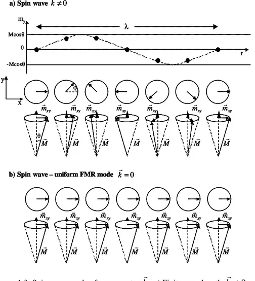
The general solutions of the linearized LLG equation are spin waves that correspond to the propagation of “small perturbations” through sample. These perturbations are

characterized by a well-defined spatial correlation of the phase ϕ and of the deviation angle or

spin wave amplitude θ (fig.1.3). In the particular case, when the magnetic moments precess in

phase in the entire magnetic system, the precession mode is uniform (ϕ = 0, θ = const.)

Figure 1.3: Spin wave mode of wave vector kr: a) Finite wavelength kr≠0

and b) uniform precession mode kr=0 (λ =∞).

The spin wave frequency carries information about system energy such as the

anisotropy energy, the external magnetic fields or the saturation magnetization (MS).

Therefore, measurements of spin wave frequencies are an important tool to characterize magnetic systems. There are two complementary types of experiments that are commonly used to study spin waves, Brillouin Light Scattering (BLS) [Cochran1995, Hillebrands1995] and FerroMagnetic Resonance (FMR) [Heinrich1995, Celinski1997, and Farle1998]. In the

BLS spin waves of wave vector kr can be created or annihilated in contrast to the FMR

excitations in which no momentum is transferred and only those modes are excited for which

the total momentum is zero, kr =0.

Besides those conventional measurements, recently new types of measurement techniques in the time domain have been presented in the literature [Silva1999, Celinski1997, Crawford1999, Freeman1992, Russek2000B], similar to the one described in this thesis. They are based on a pump-probe technique, which employs coplanar wave-guide devices and

x y Mr Mr Mr Mr Mr Mr Mr xy mr mxy r xy mr mxy r xy mr mxy r xy mr my r 0 Mcosθ -Mcosθ λ a) Spin wave kr≠0

b) Spin wave – uniform FMR mode kr=0

Mr xy mr Mr xy mr Mr xy mr Mr xy mr Mr xy mr Mr xy mr Mr xy mr ϕ θ x y Mr Mr Mr Mr Mr Mr Mr xy mr mxy r xy mr mxy r xy mr mxy r xy mr my r 0 Mcosθ -Mcosθ λ a) Spin wave kr≠0

b) Spin wave – uniform FMR mode kr=0

Mr xy mr Mr xy mr Mr xy mr Mr xy mr Mr xy mr Mr xy mr Mr xy mr x y Mr Mr Mr Mr Mr Mr Mr xy mr mxy r xy mr mxy r xy mr mxy r xy mr my r 0 Mcosθ -Mcosθ λ a) Spin wave kr≠0 x y Mr Mr Mr Mr Mr Mr Mr xy mr mxy r xy mr mxy r xy mr mxy r xy mr x y x y Mr Mr Mr Mr Mr Mr Mr xy mr mxy r xy mr mxy r xy mr mxy r xy mr my r 0 Mcosθ -Mcosθ λ my r 0 Mcosθ -Mcosθ λ a) Spin wave kr≠0 a) Spin wave kr≠0

b) Spin wave – uniform FMR mode kr=0

Mr xy mr Mr xy mr Mr xy mr Mr xy mr Mr xy mr Mr xy mr Mr xy mr

b) Spin wave – uniform FMR mode kr=0 b) Spin wave – uniform FMR mode kr=0

Mr xy mr Mr xy mr Mr xy mr Mr xy mr Mr xy mr Mr xy mr Mr xy mr Mr xy mr Mr xy mr Mr xy mr Mr xy mr Mr xy mr Mr xy mr Mr xy mr ϕ θ

allows one to determine the natural precession frequency from the damped oscillations measured in the time domain (see chapter 2).

Because, for magnetization dynamics experiments, the natural frequencies set the time-scale, we will derive in the following the uniform mode frequencies for a continuous thin film.

Uniform Ferro-Magnetic Resonance mode

The FMR technique consists of the measurement of the absorption of the microwave energy when a spatially uniform microwave (rf) magnetic field excites the magnetic moments in a system. A minimum in the microwave spectrum occurs when the rf-frequency coincides with the magnetization precession frequency.

The equation of motion of the magnetizatio n for small amplitude precessions is obtained

from the linearized Landau-Lifshitz-Gilbert equation (eq.1.18b) in the lossless case (α = 0)

[Kittel 1947].

Solutions of the linearized equation yield the precession frequency as a function of the second derivate of the energy [Farle1998, Miltat2002]:

2 2 2 2 2 2 sin _     ∂ ∂ ∂ − ∂ ∂ ∂ ∂ = ϕ θ ϕ θ θ γ γ ω E E E M (1.21) Figure 1.4:

Spherical coordinates for the magnetization and magnetic field vectors used in the calculation of the ferromagnetic resonance frequency

Using the energy expression of a continuous film of uniaxial in-plane anisotropy, one obtains the Kittel equation:

] 2 cos ) cos( ][ 4 cos ) cos( [ sin 1 2 m u H m S m u H m H M H H H ϕ ϕ ϕ π ϕ ϕ ϕ θ γ ω _{= − + + − +} (1.22)

where the angles θ, ϕm and ϕH are defined in figure 1.4. H represents the external magnetic

field whose orientation is defined by the angles ϕH and θH (here the external field is

y H M f H f M ?M ?_M x z y H M f H f M ?M ?_M x z θH θ ϕm ϕh

considered in the film plane, θH=90°), Hu represents the uniaxial anisotropy field and its

orientation is defined by θ and ϕm. The microwave field is considered to be perpendicular to

the external field.

Considering the particular case of a magnetic thin film in (x,y) plane excited by a

rf-magnetic field, Hrf, parallel to the ox-axis, in an external magnetic field, H, parallel to

oy-axis, the magnetic susceptibility associated to the rf- magnetic field is defined as:

2 0 1     − = = ω ω χ χ H rf x rf H M (1.23) where H My H =

χ . We observe that the variation of the magnetic susceptibility as a function

of ω, has a maximum for ω =ω₀. The imaginary parts of the magnetic susceptibility, Im(χm) characterize the energy absorption that appears in the magnetic system due to excitation by an

rf-magnetic field. The absorbed microwave power, Prf, in a magnetic thin film, is defined as

[Celinski 1997]:

[ ]

2 Im 2 1 rf rf rf H P = ω χ ⋅ (1.24)

For an external rf-magnetic field of frequency f =ω 2/ π equal to the frequency

π ω 2₀/

0 =

f of the magnetization precessions, the rf-energy is entirely absorbed by the

magnetic system. The frequency f0 is called the ferromagnetic resonance frequency.

Ferromagnetic resonance occurs for the frequency value for which the absorbed power in the thin film (eq.1.24) is at maximum value.

1.5. MAGNETIC LENGTHSCALES

Coming back to the static magnetization distribution, there exist different magnetic length scales that characterize the magnetic static distribution. These length scales are derived from the competition between the internal energies of the system (defined in section 1.2), the exchange, magnetostatic, and magneto-crystalline energies.

• The competition between the exchange energy and the anisotropy energy defines the

K A_ex

=

∆0 (1.25)

• The competition between the exchange energy and the magnetostatic energy defines the

exchange length: 2 0 2 S ex ex M µ A l = (1.26)

• The quality factor compares the magneto-crystalline to the magnetostatic energy:

2 0 2 S M µ K Q= (1.27) 1.6. DOMAIN WALLS

Barkhausen found the first experimental confirmation of the magnetic domain concept in 1919 [Barkhausen1919]. He discovered that the magnetization process in an applied field contains discontinuous variations named Barkhausen jumps, which he explained as magnetic

domain switching4. Further analysis of the dynamics of this process [Sixtus 1931] led to the

conclusion that such jumps can occur by the propagation of the boundary between domains of opposite magnetization.

In 1932, Bloch [Bloch1932] analyzed the spatial distribution of the magnetization, M, in the boundary regions between domains, finding that they must have a width of several hundred lattice constants, since an abrupt transition (over one lattice constant) would be in conflict with the exchange interaction. Two basic modes of the rotation of the magnetization vector can be defined for domain walls:

i) The three dimensional (3D) rotation of the magnetization from one domain through a 180° wall to the other domain, determining a Bloch wall (fig.1.5a). Here the magnetization rotates in a plane parallel to the wall plane. This wall is characteristic to bulk materials or thick films.

ii) The two dimensional (2D) rotation of the magnetization from one domain through a 180° wall to the other domain, determining a Néel wall. Here the magnetization rotates perpend icular to the wall plane. This type of walls appears in thin magnetic films, where the in-plane rotation of the magnetization has a lower energy than in the classical Bloch wall

4

mode (fig.1.5b). This is due to the demagnetizing field produced by the Bloch wall spins that point perpendicular to the film surface. In order to reduce these fields, the magnetization starts to rotate in-plane.

The transition from a Bloch wall to a Néel wall occurs roughly when the film thickness, t, becomes comparable to the wall width, δw. (Hubert1998).

Figure 1.5:

180° magnetic domains walls:

(a) Bloch walls in a bulk material (b) Néel walls in a thin magnetic film

The width of a domain wall (δw) is proportional to Bloch parameter, (∆0) defined in

equation 1.25. The Néel wall is thinner than the Bloch walls Bloch

w Néel

w δ

δ < where the width of

a Bloch wall can be estimated by:

0

∆

=π

δBloch

w (1.28)

1.7. MAGNETIZATION REVERSAL MECHANISMS

As a function of the sample dimensions and the type of excitation fields (static or pulsed, of variable sweep rate – dH/dt, of different orientations with respect to the uniaxial anisotropy) one distinguishes between different classes for the magnetization reversal processes, for which the most important ones are detailed below:

i) Reversal obtained by nucleation and domain wall propagation ii) Reversal by uniform rotation of the magnetization

iii) Reversal by magnetization precession

(a) t > δ_w t w w (b) t < δ_w t δ_w ∈(10 nm –hundreds of nm) δw δw (a) t > δ_w t w w (b) t < δ_w t δ_w ∈(10 nm –hundreds of nm) δw δw

1.7.1. DOMAIN WALL DYNAMICS

The first magnetizatio n curve and the hysteresis loop of an extended ferromagnetic material (note: this does not hold necessarily for nanomagnets) characterize the quasi-static reversal of its magnetization (fig1.6) in a varying external magnetic field. On the first magnetization cur ve (fig.1.6), the magnetization alignment parallel to the external field is realized by reversible wall displacements and non-coherent rotation from point A to point B and then by coherent rotation from B to the saturation point C [Kittel1966]. Wall displacement increases the magnetic domain surface that has the magnetization parallel to the external magnetic field and consequently, decreases the magnetic domain with the magnetization anti-parallel to the external magnetic field [Koch1998, Choi2001].

On the hysteresis curve, decreasing the external field from positive saturation (point C), the nucleation of reversed magnetic domains sets in at a certain value of the magnetic field as we can observe in point D on figure 1.6. Depending on the sample type and magnetic homogeneity, the dynamics from the point D to F may include domain wall displacements, and non-coherent or coherent magnetization rotations.

Figure 1.6

Magnetic domain configuration corresponding to different points on the first magnetization curve and hysteresis loop

-20 0 20 40 60 -1,0 -0,5 0,0 0,5 1,0 E F D C B A b a

a: first magnetization curve b: hysteresis loop M H(u.a) H B H B B Magnetic domain Domain wall i Mr A H = 0, ΣMi= 0 Magnetic domain Domain wall i Mr Magnetic domain Domain wall i Mr A H = 0, ΣMi= 0 E H E H F H ≥ -H_sat F H ≥ -H_sat C H ≥ Hsat C H ≥ Hsat D H D H -20 0 20 40 60 -1,0 -0,5 0,0 0,5 1,0 E F D C B A b a

a: first magnetization curve b: hysteresis loop M H(u.a) H B H B B Magnetic domain Domain wall i Mr A H = 0, ΣMi= 0 Magnetic domain Domain wall i Mr Magnetic domain Domain wall i Mr A H = 0, ΣMi= 0 E H E H F H ≥ -H_sat F H ≥ -H_sat C H ≥ Hsat C H ≥ Hsat D H D H

One important parameter that characterizes the domain wall propagation in the presence of an external magnetic field is the wall velocity, v. This velocity can be deduced by integrating the Landau-Lifshitz-Gilbert equation (1.18b) over the domain wall width [Malozemoff1979, Hubert1998]. Since the displacement mechanism of a Bloch wall has some similarities to the precessional reversal process (detailed in section 1.7.3) it will be detailed in the following.

We suppose two neighboring magnetic domains with their magnetizations “up” and “down” separated by a 180° Bloch domain wall. The Bloch wall magnetization is oriented in the wall plane and perpendicular to the domain magnetization. An “up” magnetic field exerts no torque on the domain magnetization since the angles between the field and the domain magnetization vectors are 0° and 180°, respectively. Contrary, the torque between the domain

wall magnetization and the external field (Mr_wall×Hr ) rotates the magnetization out of the

wall plane by an angle ϕwall, from point 1 to point 2 as shown in the figure 1.7. This creates a

strong demagnetizing field, hd, perpendicular to the wall plane, which induces a precession of

the magnetization around hd, rotating the magnetization from point 2 to point 3.

Consequently, the wall magnetization aligns with the domain magnetization that is parallel to the external field. This is equivalent to a wall propagation from left to right in figure 1.7 with the velocity v.

Figure 1.7

a) Ferromagnetic structure composed of magnetic domains and domain walls; b) Bloch wall displacement mechanism

The domain wall velocity, v, is proportional to the difference between the external field,

HA, and the coercive field, HC, to the sample magnetization, MS, to the wall width

vr ext Hr + + + + + + + + + -- -d hr ext Hr + + + + + + + + + -- -1 2 3 vr ext Hr + + + + + + + + + -- -d hr ext Hr + + + + + + + + + -- -d hr ext Hr + + + + + + + + + -- -ext Hr + + + + + + + + + -- -1 2 3 Magnetic domain Domain wall i Mr Magnetic domain Domain wall i Mr a) b) ϕwall

(≈ A_ex K ), to the gyromagnetic factor, γ, and is inversely proportional to the damping parameter λ [Doyle 1998]:

(

A C

)

ex S H H µ K A M v∝ ⋅ ₀ − λ γ (1.29)

Equation 1.29 can be rewritten to obtain a more general expression for the reversal time,

τ:

(

)

(

)

µ L A K M L S H H S µ H H µ K A L M L v ex S w C A w C A ex S = = − = − ⋅ ∝ = γ λ λ γ τ with ; 1 0 0 (1.30)

The parameter Sw represents the switching coefficient and it is defined as the ratio

between the sample length, L, and the effective wall mobility, µ. These relations have been verified by numerous experiments in the past for larger (bulk) samples [Rado 1963].

It is noted that the reversal mechanism depends on the external magnetic field sweep rate (dH/dt). For example, Camarero et al [Camarero2001] studied the influence of the external field sweep rate (dH/dt) on the magnetization reversal dynamics. They revealed that the magnetization reversal is dominated by domain wall displacements for low dH/dt values and by nucleation processes for higher dH/dt values in exchange coupled NiO -Co bilayers.

A nice parallel between the reversal of cluster particles of variables densities on the substrate and the reversal dominated by domain dynamics in thin films [Ferre1997] was experimentally realized in 2003 by Binns et al. [Binns2003]. He showed that at low coverage of the substrate with clusters, the switching dynamics of the sample remains the same as in the clean substrate while above a certain limit of coverage, a significant acceleration of the magnetic reversal was observed with a fast component due to a reversal propagating through the cluster film. Its conclusion was that the velocity of the propagation, rather than the rate of reverse magnetization nuclei, dominates the reversal through the cluster film, the average

1.7.2. COHERENT MAGNETIZATION REVERSAL –STONER-WOLFARTH MODEL

The coherent rotation model was developed by Stoner-Wolfarth [St.-W. 1948] and Louis Néel [Néel 1947]. This model considers the magnetization reversal of a mono-domain particle in an external magnetic field, H. In this case, the rotation of the magnetic moments increases the anisotropy energy while the exchange energy remains constant.

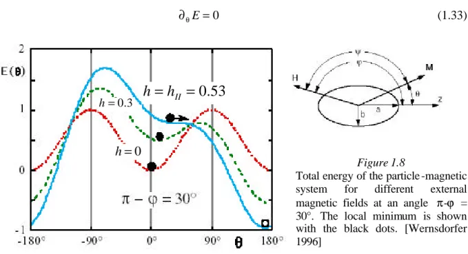
Figure 1.8 shows the evolution of the mono-domain particle energy as a function of the

applied magnetic field, H, which defines the equilibrium angle θ of the magnetization

direction with respect to the uniaxial anisotropy easy axis. The total energy of the particle is the sum over three terms: the demagnetization, Zeeman, and magneto-crystalline energies. The normalized energy is written as [Wernsdorfer 1996]:

( )

θ −

(

θ −ϕ

)

=sin2 2 cos h

E (1.31)

where the angles θ and ϕ are specified in figure 1.8, and h represents the ratio between the

external field energy and the magneto-crystalline anisotropy energy constant, K:

K MH µ H H h K 2 0 = = (1.32)

We consider the particle to be in one of the energy minima at zero field, as shown in figure 1.8 on the symmetric curve for h = 0. This corresponds to the magnetization parallel to the easy axis of the particle where the first derivate of the energy function is zero:

0

=

∂_θE (1.33)

Figure 1.8

Total energy of the particle -magnetic system for different external magnetic fields at an angle π-ϕ = 30°. The local minimum is shown with the black dots. [Wernsdorfer 1996]

Applying a magnetic field into the opposite direction of the magnetization the symmetric curve becomes asymmetric and the local energy minimum moves toward positive

53

.

0

=

=

h

II

h

3 . 0 = h 0 = h

53

.

0

=

=

h

II

h

3 . 0 = h 0 = h

53

.

0

=

=

h

II

h

3 . 0 = h 0 = h

angles θ. Increasing the field values, the difference between the energy minimum and energy

maximum is decreasing going to zero at a critical magnetic field, hc. This corresponds to a

saddle point where the second derivate of the energy is zero:

0 2 =

∂_θE (1.34)

From (1.31 – 1.33) we obtain an expression of the critical reversal field, hc, as a function

of the angle ϕ between the direction of the applied field and the uniaxial anisotropy direction:

(

_{2/3 2/3}

)

3/2 cos sin 1 ϕ ϕ+ = c h (1.35)

The angle θ0 defined as the angle between the magnetization M

r

and the direction oz, for which the magnetization reversal occurs, can be expressed as:

ϕ

θ 1/3

0 tan

tan =− (1.36)

The critical field, hc, for which the reversal occurs as a function of the angle ϕ, (eq.1.36)

is presented by the Stoner-Wolfarth astroid in figure 1.9. The curve hr =hr₀

( )

ϕ delimitates the

region of reversal (hr≥hr₀

( )

ϕ ) from the region of non-reversal (hr <hr₀

( )

ϕ ).

Figure 1.9

Stoner-Wolfarth astroid that defines the limit between the non-reversal (inner region) and reversal (outer region) regions.

Referring to figure I.1 from the general introduction, this process appears in single-domain magnetic systems, where quasi-static external fields are applied parallel to the direction to which the magnetization should be reversed.

Wernsdorfer et al. experimentally verified the Stoner-Wolfarth model on magnetic nanoparticles of 50-150nm dimensions. Despite a clear single-domain character of the particles, they showed that a distribution of switching field exists, whose width increases by decreasing the temperature and becomes constant at very low temperatures [Wernsdorfer

0 30 60 90 120 150 180 210 240 270 300 330

( )

ϕ

0

h

r

H_z H_y 0 30 60 90 120 150 180 210 240 270 300 330

( )

ϕ

0

h

r

0 30 60 90 120 150 180 210 240 270 300 330

( )

ϕ

0

h

r

H_z H_y

1995]. For non-zero temperatures, the switching field becomes a stochastic variable and the magnetization switching takes place before the energy barrier goes to zero [Bonet 1999, Thirion 2002].

Stoner-Wolfarth reversal is actually used in MRAM applications (see FIMS – fig.I.3 – general introduction), the magnetic memory being reversed by the total field obtained with

two magnetic field pulses (Hy and Hz in figure 1.9) obtained with two conductor lines

perpendicular to each other. The time scales, characteristic to this reversal, are in the nanosecond range.

In order to understand the time limits that occur during the coherent rotation reversal, we consider a Stoner-Wolfarth particle represented by an ellipsoid with the long axis parallel to the oy-axis. We will analyze the details that appear during the coherent rotation of the magnetization toward an external magnetic field applied parallel to this oz-axis as shown in figure 1.10. We suppose that the amplitude of the external magnetic field is slowly increased

up to the anisotropy field value (Hk). This means that for each value of the external magnetic

field (7 values on figure 1.10) the magnetization “has the time” to relax parallel to its current effective magnetic field.

Figure 1.10

Quasi-static relaxation of the magnetization during its reversal by coherent rotation in a Stoner-Wolfarth particle

For H = 0 the magnetization is parallel to the oy-axis position that corresponds to one local minimum of the symmetric curve from figure 1.10. Increasing the magnetic field from

zero to 0.1HK (applied parallel to +oz axis) the angle corresponding to the local minimum

varies from 0° to about 10°, corresponding to the new orientation of the effective field. The magnetization relaxes into this new local minimum executing a small- angle precessional

H=0 H=0 M M -60 0 60 120 180 240 -2 -1 0 1 2 3 4 Angle (deg) Energie (a.u.) H = 0.1 H = 0.1HH_kk H = 0.5 H = 0.5HH_kk H = 0.2 H = 0.2HHkk H = 0.3 H = 0.3HH_kk H = 0.7 H = 0.7HH_kk H = 1.0 H = 1.0HH_kk K K_uu H=0 H=0 M M -60 0 60 120 180 240 -2 -1 0 1 2 3 4 Angle (deg) Energie (a.u.) -60 0 60 120 180 240 -2 -1 0 1 2 3 4 Angle (deg) Energie (a.u.) H = 0.1 H = 0.1H = 0.1HH_kk H = 0.1HH_kk H = 0.5 H = 0.5H = 0.5HH_kk H = 0.5HH_kk H = 0.2 H = 0.2H = 0.2HHkk H = 0.2HHkk H = 0.3 H = 0.3H = 0.3HH_kk H = 0.3HH_kk H = 0.7 H = 0.7H = 0.7HH_kk H = 0.7HH_kk H = 1.0 H = 1.0H = 1.0HH_kk H = 1.0HH_kk K K_uu z y H=0 H=0 M M -60 0 60 120 180 240 -2 -1 0 1 2 3 4 Angle (deg) Energie (a.u.) H = 0.1 H = 0.1HH_kk H = 0.5 H = 0.5HH_kk H = 0.2 H = 0.2HHkk H = 0.3 H = 0.3HH_kk H = 0.7 H = 0.7HH_kk H = 1.0 H = 1.0HH_kk K K_uu H=0 H=0 M M -60 0 60 120 180 240 -2 -1 0 1 2 3 4 Angle (deg) Energie (a.u.) -60 0 60 120 180 240 -2 -1 0 1 2 3 4 Angle (deg) Energie (a.u.) H = 0.1 H = 0.1H = 0.1HH_kk H = 0.1HH_kk H = 0.5 H = 0.5H = 0.5HH_kk H = 0.5HH_kk H = 0.2 H = 0.2H = 0.2HHkk H = 0.2HHkk H = 0.3 H = 0.3H = 0.3HH_kk H = 0.3HH_kk H = 0.7 H = 0.7H = 0.7HH_kk H = 0.7HH_kk H = 1.0 H = 1.0H = 1.0HH_kk H = 1.0HH_kk K K_uu z y