HAL Id: tel-02521809
https://tel.archives-ouvertes.fr/tel-02521809
Submitted on 27 Mar 2020
HAL is a multi-disciplinary open access
archive for the deposit and dissemination of sci-entific research documents, whether they are pub-lished or not. The documents may come from teaching and research institutions in France or abroad, or from public or private research centers.
L’archive ouverte pluridisciplinaire HAL, est destinée au dépôt et à la diffusion de documents scientifiques de niveau recherche, publiés ou non, émanant des établissements d’enseignement et de recherche français ou étrangers, des laboratoires publics ou privés.
Elias Bouacida
To cite this version:
Elias Bouacida. Choices, Preferences, and Welfare. Economics and Finance. Université Panthéon-Sorbonne - Paris I, 2019. English. �NNT : 2019PA01E017�. �tel-02521809�
Université Paris I Panthéon Sorbonne
UFR d’Economie
Laboratoire de rattachement: Paris Jourdan Sciences Economiques
THÈSE
Pour l’obtention du titre de Docteur en Sciences Economiques
Présentée et soutenue publiquement
le 10 juillet 2019 par
Elias Bouacida
Choices, Preferences, and Welfare
Sous les directions de :
Jean-Marc Tallon, Directeur de recherche CNRS, PjSE, Professeur à l’école d’économie de Paris Daniel Martin, Associate Professor, Kellog School of Management, Northwestern University Jury :
Rapporteurs :
Eric Danan, Chargé de recherche CNRS – HDR, THEMA, Université de Cergy-Pontoise Georgios Gerasimou, Senior Lecturer, Université de Saint-Andrews
Examinateurs :
Olivier l’Haridon, Professeur à l’université de Rennes
Contents
Remerciements 9
1 Introduction 11
1.1 Revealed Preferences . . . 14
1.2 Beyond Classical Preferences . . . 20
1.2.1 Relaxing Transitivity and Menu-Independence . . . 22
1.2.1.1 Partial Order . . . 24 1.2.1.2 Interval Order . . . 25 1.2.1.3 Semi-Order . . . 25 1.2.1.4 Monotone Threshold . . . 26 1.2.1.5 Menu-Dependent Threshold . . . 26 1.2.1.6 Context-Dependent Threshold . . . 27
1.2.2 Robust Revealed Preferences . . . 27
1.2.2.1 The Strict Unambiguous Choice Relation . . . 29
1.2.2.2 The Transitive Core . . . 30
1.2.2.3 Other Welfare Relations . . . 30
1.3 Organization of the Dissertation . . . 31
2 Predictive Power in Behavioral Welfare Economics 33 2.1 Introduction . . . 33
2.1.1 Empirical Findings in Behavioral Welfare Economics . . . 37
2.2 Data . . . 38
2.2.1 Experimental Data . . . 39 3
2.2.2 Consumption Data . . . 40
2.2.2.1 Analysis Sample: Panelists . . . 40
2.2.2.2 Analysis Sample: Demographic Characteristics . . . 41
2.2.2.3 Analysis Sample: Bundles . . . 42
2.2.2.4 Analysis Sample: Prices . . . 43
2.2.2.5 Additional Considerations . . . 45
2.3 Results . . . 45
2.3.1 Inconsistencies in Revealed Preferences . . . 45
2.3.2 Inconsistencies in SUCR and TC . . . 46
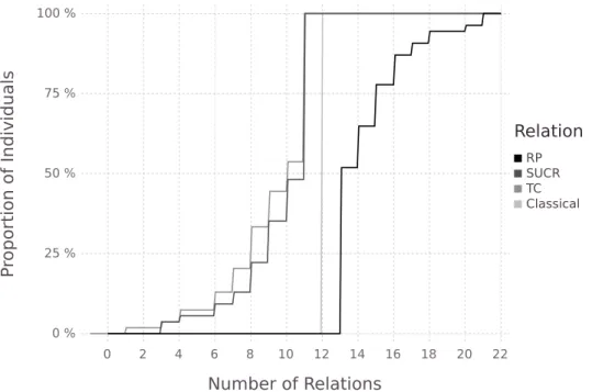
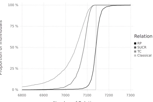
2.3.3 Completeness of SUCR and TC . . . 47
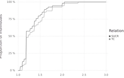
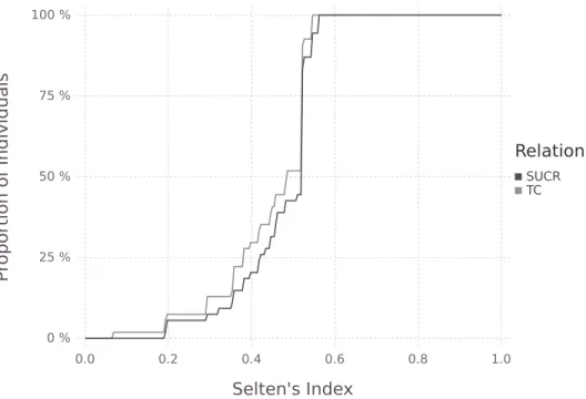
2.3.4 Predictive Power of SUCR and TC . . . 49
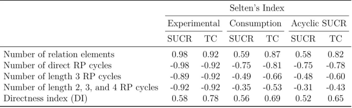
2.3.5 Predictive Power and Revealed Preference Properties . . . 52
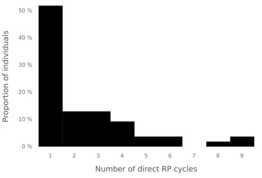
2.3.5.1 Number of Direct RP Cycles . . . 54
2.3.5.2 Fraction of RP Cycles that are Direct . . . 55
2.3.5.3 Regression Analysis . . . 56
2.4 Discussion and Conclusion . . . 56
3 Identifying Choice Correspondences 59 3.1 Introduction . . . 59
3.2 Deinition of the Pay-For-Certainty Method . . . 63
3.2.1 General Setup . . . 63
3.2.2 Deinition of the Pay-For-Certainty Method . . . 64
3.2.2.1 Incentive to Choose Several Alternatives . . . 65
3.2.2.2 Selection Mechanisms . . . 66
3.2.2.3 Linear versus Proportional Bonus Payment . . . 68
3.2.3 Pay-For-Certainty with a Uniform Selection Mechanism . . . 68
3.3 Identiication of the Choice Correspondence . . . 69
3.3.1 Assumptions . . . 69
CONTENTS 5
3.3.2.1 Partial Identiication of the Choice Correspondence . . . 72
3.3.2.2 Full Identiication of the Choice Correspondence . . . 74
3.3.3 Consistency when Full Identiication Fails . . . 75
3.3.3.1 Compatibility with Classical Preferences . . . 76
3.3.3.2 Compatibility with a Partial Order . . . 79
3.3.3.3 Compatibility with Menu-Dependent Threshold . . . 81
3.3.3.4 Compatibility with Fixed Point . . . 82
3.4 Conclusion . . . 82
4 Pay-for-certainty in an Experiment 85 4.1 Introduction . . . 85
4.1.1 Menu Choice in the Literature . . . 88
4.2 Design of the Experiment . . . 89
4.2.1 Tasks . . . 90 4.2.2 Timing . . . 91 4.2.3 Information Treatments . . . 92 4.2.4 Choices . . . 92 4.2.5 Questionnaire . . . 94 4.2.6 Data . . . 94 4.2.7 Demographics Characteristics . . . 94
4.3 Comparing Three Revelations Method . . . 95
4.3.1 The Benchmark: Forced Single Choice . . . 95
4.3.2 0-Correspondences . . . 97
4.3.3 1-Correspondences . . . 98
4.3.4 Identiied Choice Correspondence . . . 99
4.3.4.1 Fully Identiied Choice Correspondences . . . 100
4.3.4.2 Partially Identiied Choice Correspondences . . . 101
4.3.5 Related Literature and Discussion . . . 101
4.4.1 Intransitive Indiference . . . 103
4.4.2 Menu-Dependent Choices . . . 104
4.4.3 Discussion . . . 104
4.5 Inluence of the Information Provided . . . 105
4.6 Conclusion . . . 109
5 Conclusion 111 A Appendix of Chapter 2 113 A.1 Choice Set Size . . . 113
A.2 Correlations for Uniform Random Demands . . . 113
A.2.1 Uniform Random Methodology: Consumption Data . . . 113
A.2.2 Uniform Random Methodology: Experimental Data . . . 114
A.2.3 Results . . . 114
B Appendix of Chapter 3 117 B.1 Own Randomization . . . 117
B.2 Extending Pay-For-Certainty to Ininite Sets . . . 119
B.2.1 Ininite Choice Sets . . . 119
B.2.2 Finite Choice Sets on Ininite Sets . . . 120
C Appendix of Chapter 4 121 C.1 Design . . . 121
C.1.1 Tasks . . . 121
C.1.2 Instructions . . . 124
C.1.2.1 Gains in the experiment . . . 124
C.1.2.2 Remarks . . . 124
C.1.2.3 Instructions . . . 125
C.2 Explanatory Power of Diferent Axioms . . . 126
C.3 Size of the Chosen Sets . . . 127
CONTENTS 7
C.4.1 With Forced Single Choice . . . 129
C.4.2 0-Correspondences . . . 130
C.5 Results with High Payments . . . 131
C.6 Choice Functions and Choice Correspondences on the Same Subjects . . . 133
C.7 Aggregating Choices . . . 134
C.7.1 Information and Maximal Alternatives . . . 134
C.7.2 An Alternative Determination of Maximal Alternatives . . . 135
D Analytical Computer Programs 139 D.1 Chapter 2 . . . 139
D.2 Chapter 4 . . . 139
Bibliography 139 E Résumé en Français 153 E.1 Introduction . . . 153
E.2 Pouvoir prédictif en économie du bien-être comportementale . . . 157
E.3 Identiication des correspondances de choix . . . 162
E.4 Payer pour la certitude dans une expérience . . . 166
Remerciements
I am thankful to my colleagues, my family, and my friends, who supported me and helped me for the last ive years and beyond! Without you, this Ph.D. would not look the same.
Je tiens à remercier mes collègues, ma famille et mes amis, qui m’ont aidé et soutenu tout au long de ces cinq dernières années, et bien plus ! Sans vous, cette thèse ne sera pas ce qu’elle est.
I want to thank Daniel Martin, who lead my irst steps in research. You were and still are crucial support, and I have really enjoyed working under your direction, and now with you. You are also the one who recommended me to Jean-Marc Tallon, which may be the single most signiicant result of my master thesis dissertation.
Jean-Marc Tallon, merci ! Merci pour ta porte toujours ouverte, ta disponibilité et ton soutien sans faille, ta gentillesse, et surtout, tes commentaires toujours pertinents, même si j’ai parfois mis du temps à les comprendre… Cette thèse te doit aussi beaucoup et ces cinq années auraient été très diférentes sans toi.
J’aimerai aussi remercier Stéphane Zuber, qui a suivi cette thèse de près. Ta rigueur et tes com-mentaires ont toujours été pertinents et m’ont toujours éclairé.
I would like to thank the members of my jury, who accepted to spend time on my thesis and have already given me great comments. Eric Danan, in particular, was available way before the jury took shape, and talking with you was always very fruitful, at the MSE, Cergy or PSE.
To all the researchers I had the chance to talk with during my Ph.D., at the MSE, PSE, Northwest-ern, and Nanterre in particular, thank you! Nicolas Jacquemet and Béatrice Boulu-Reshef’s advice, as well as all the workgroup in experiments, have been of great help when I started building my experiment, and well after. Maxim Frolov is an excellent and dedicated lab’ programmer, without him, I would have lost a ton of time running my irst experiment. I have participated in many conferences and seminars during my Ph.D., thanks to the administrative support at MSE and PSE for making the process smoother. All the participants in these conferences make the process of research more collaborative and more enjoyable.
On that note, I would like to thank all the researchers, Ph.D. and administrative staf involved in the job market training, without whom I would not have gotten the job at Lancaster. Véronique
Guillotin in particular, who was and is always available for Ph.D. students, and who shared the good and the bad news of all of us. Eyal Winter and Maurizio Zanardi allowing me to pursue my research interest in the next three years at Lancaster University. I am eager to come!
The discussion, support, and presence of my colleagues and friends were all integral and essential part of the last ive years. To name a few and forgetting many more. My oicemates: Thomas, Juliette, Aya, Joanna, Ariane, Emanuela, Sasha, Sulin, Cem, Annali, Alexia, Maiting, Avner, Ezgi, Ole, Florian, Peio, Zouhair, Anthony, Dalia, George, Sandrine, Julianna. My colleagues and lunch mates: Giulio, Guillaume, Shaden, Julien, Rémi, Léontine, Anna, Justine, Antoine, An-toine, Matthieu, Alexandra, Simon, Philippe, Juni. The two reading groups: Simon, Rémi, Avner, Philippe, Quentin, Anthony, and Niels. Paul and Juliette, the team of committed representatives. To the Synapse members over the years, and in particular, Julien, Zahra and Juni. A special thank for Zahra, who made my arrival and my life in Chicago much, much more relaxed and funnier! All of you, and many others, have made my Ph.D. more fruitful and more enjoyable, in one way or another, thank you!
Ma famille, mes proches et mes amis. Ces cinq dernières années n’ont pas toujours été faciles. Merci d’avoir été là, votre soutien a été, est et sera toujours essentiel. Merci à Quentin, Benjamin, Claire, Pierre, Maxime, Clément, Marion, Andéol, Johan, Roman, pour nos super week-ends, et ce n’est pas ini : votre prochaine destination, c’est Lancaster ! Merci à Lucile, nous avons commencé nos doctorats en même temps, et nous allons les inir presque en même temps ! Merci à Inès, Inès, Haïfa, Sabrine et Youssr, mes tunisiens en France, il y a des choses que vous seules comprenez. Grand merci à Alter’Actions, et en particulier, Isabelle, Michel, Benjamin, Francesca, Amandine, Nicolas et Audrey, vous m’avez rattaché à une réalité diférente de la recherche cinq années durant, qui m’ont aidé à garder les pieds sur terre. Merci à une des parties les plus stable de ma vie jusqu’à présent, le karaté, et en particulier, Senseï, Léa, Laurant, Philippe, Carlos, Vuslat, Pierre, Lahcène, Jean, Catherine, et tous les autres. Vous m’avez aussi rattaché à un monde diférent de la recherche et vous allez me manquer. Merci à mes colocs des 10 dernières années.
Ma famille, et en particulier mes cousins et cousines, vivant à Paris n’est pas et n’a pas été très nombreuse au cours de ces années, mais est toujours d’un grand soutien. Grâce à vous, je me sens plus chez moi à Paris ! Un remerciement particulier à Inès, qui a déjà vécu une thèse avant la sienne. Maintenant, je t’en dois une !
Chapter 1
Introduction
This dissertation studies the link between choices, preferences, and individual welfare. One object of interest in this dissertation is an alternative. An alternative can take various forms; it may be a bundle purchased from the supermarket, a meal, the possibility to register in a university, the date to which you will have dinner with your parents. Choices are made between diferent alternatives. Preferences are a ranking of the alternatives to choose from. Welfare is the well-being, or satisfaction, obtained from an alternative.
The assessment of welfare is an integral part of economics, in particular for the evaluation of public policy and policy recommendations. One method to study individual welfare is to identify the satisfaction decision makers retain from their choices. It can be a relative or an absolute satisfaction, and it can be obtained by directly asking, for instance, in subjective well-being studies, or by deducing it from the preferences of individual decision makers. Preferences are not directly observable, but they can be inferred. The principle we will use in this dissertation was introduced by Samuelson (1938)’s seminal paper; it is called revealed preferences. Revealed preferences link choices and preferences. Little (1949) was the irst to propose to use revealed preferences for individual welfare analysis.
There is an apparent contradiction between Samuelson (1938)’s project with revealed preferences and Little (1949)’s use of revealed preferences for welfare analysis. Indeed, Samuelson (1938)’s analysis stated aim was (emphasis are ours):
I propose, therefore, that we start anew in direct attack upon the problem, dropping of the last vestiges of the utility analysis.
If indeed, revealed preferences aimed at dropping any trace of utility in economic analysis, it would not be suitable for welfare analysis, as the revealed preference would not represent anything mean-ingful from a welfare perspective. It would only be an as if tool to model choices made by decision
makers, a convenient mathematical representation to represent choices made. Little (1949)’s words (the theory of consumer behavior should be understood as the revealed preference theory):
In the theory of Consumer’s Behaviour, as at present formulated, the preferences (in the subjective sense) which are discovered by asking questions are linked to market behaviour by the postulate that people do in fact try to maximize satisfaction. It is thus false to suppose that the theory, as it stands at present, is concerned only with choice. It is concerned also with likes and dislikes.
Little (1949) links choices with satisfaction. It can only be understood as decision makers have a utility or a preference, which they maximize. Revealed preferences try to recover this utility from the observed choices. In Amartya Sen (1973)’s words:
The rationale of the revealed preference approach lies in this assumption of revelation and not in doing away with the notion of underlying preferences, despite occasional noises to the contrary.
To summarize, using revealed preferences for welfare analysis requires two things. First, that decision makers have a preference (utility), which is the right guide to their welfare, and second, that revealed preferences identify it. To understand whether these assumptions are warranted, it is helpful to understand the core idea of revealed preferences. It is quite intuitive. If John chooses an apple instead of a banana when both are available, then he probably prefers apples to bananas. Thus, he is better of with an apple rather than a banana. In this simple example, we can go directly from choices to welfare. Preferences are needed because not all choices are observed. If we observe that John chooses apples over bananas, and bananas over oranges, and think in terms of welfare, we probably expect him to choose apples over oranges, even without observing a choice between apples and oranges.
While intuitively straightforward, the reasoning faces hurdles in practice. For instance, what should we conclude if John sometimes chooses bananas and sometimes apples, or if he chooses apples over bananas, bananas over oranges, and oranges over apples? It is harder to reveal a preference with a welfare interpretation in these cases. The second problem is that the preference built from observed choices might not be the one we should use for welfare analysis. What should we think of the choices of a smoker choosing to smoke, while knowing that it is unhealthty, for instance? The use of choices as a guide to welfare is has been debated for a long time, in diferent forms. Amartya Sen (1973), for instance, provides an early critique. One of the most recent iterations of this debate is in behavioral welfare economics, between, for instance, Bernheim and Rangel (2009) and Salant and Rubinstein (2008). We will come back to this last debate in Chapter 2. Mongin and d’Aspremont (1998) provide a normative defense of revealed preferences for welfare analysis.
13 If we accept that we can use choices as a guide to welfare, in the strong sense implied by revealed preferences, we still have a positive problem, like the lack of transitivity in practice. Koo (1963) provided the irst example, Choi, Fisman, et al. (2007), Choi, Kariv, et al. (2014), Dean and Martin (2016), among others, provide more recent illustrations. In those cases, it is much less straight-forward how to build a preference from observed choices, let alone think about welfare. Revealed preferences require some consistency between observed choices to be used in welfare analysis. In other words, choices must obey some rules so that we can build a preference. Indeed, if there are no rules to the observed choices, then there is no hope to build a model to explain the choices. Because the conditions implied by the rules are violated in practice, it means that the process we assume is not the right one.
There are two possible reactions to these failures. The irst is to consider that the revealed preference approach is doomed and to try to bring insights on the decision-making processes to build a more accurate model of decision making. The second is to look at the hypotheses behind revealed preferences and the setup employed and to look at why revealed preferences seem to fail. The main objective of this dissertation is to improve the revelation of preferences, and we will take these two directions to do so.
First, the revealed preference approach assumes that decision makers can be modeled as if they maximize a preference. It is not how decisions are made in general, as research in psychology and behavioral economics have shown. So revealed preferences is not a good model of the human decision making processes. Instead, decision makers can be described as using heuristics to make choices, a fact we have known at least since Tversky and Kahneman (1974). This understanding led to the development of behavioral economics. Behavioral economics usually keeps the choice as relevant to welfare analysis, even knowing that the revealed preference might not be the preference, and indeed, the preference might not exist.
The study of welfare in behavioral economics was often made using ad hoc models of the heuristics used to make choices, in order to tease out the preference from noisy choices. This kind of ap-proaches has been criticized because of their ad hoc nature. Behavioral welfare economics emerged in response, following the seminal papers of Bernheim and Rangel (2009) and Salant and Rubinstein (2008). This literature aims is to provide a more rigorous basis for the study of welfare when choices are not the results of utility maximization. So far, the literature on the topic has been primarily theoretical (Ambuehl, Bernheim, and Lusardi (2014), Bernheim, Fradkin, and Popov (2015) are two exceptions). This dissertation aims at providing empirical insights into the study of welfare in the presence of biases. In Chapter 2, with my co-author Daniel Martin, we study two propositions from the behavioral welfare economics literature.
Chapter 3 provides a method to study revealed preferences using a broader method compared to the empirical studies done so far by extending the domain of choice. It reveals some limits from the current practices of revealed preferences, and notably the possible underestimation of indiference
with the current methods. It might explain why decision makers seem sometimes mistaken in traditional experiments. Chapter 4 illustrates the method of Chapter 3 with an experiment. Section 1.1 introduces in more details the revealed preference approach, as well as the conditions for welfare assessment. Section 1.2 goes beyond the classical revealed preference approach while keeping its central insight.
1.1 Revealed Preferences
Economists traditionally model decisions made by individuals as the result of preference maximiza-tion, or, often equivalently, utility maximization. A utility is a function from the set of alternatives to the real numbers, which implies a ranking over the alternatives. The maximization is the process used to determine the alternative chosen: it should be the highest ranked according to the preference or the alternative which yield the highest utility. This strong link between the observed choice and the unobserved preference suggest that we can recover the preference or utility from the observed choices. It is the idea behind revealed preferences. Amartya Sen (1997) discusses the weaknesses of this approach, which is still a backbone of economic analysis. We use some departure of the process of utility maximization in this dissertation, but we still assume that choices relect preferences. Indeed, the process of utility maximization yields some conditions on the choices. These conditions difer depending on the choice environment. The conditions on ininite data (typically, consump-tion data, i.e., choices with quantities and prices), were irst given by Ville and Newman (1951), Houthakker (1950) and Afriat (1967)’s Weak Axiom of Revealed Preferences, and Hal R. Varian (1982)’s General Axiom of Revealed Preferences. Crawford and De Rock (2014) and Adams and Crawford (2015) are recent reviews on revealed preferences methods with consumption data and beyond. The conditions on inite data (typically, experimental data, i.e., the choice of items from a set of available alternatives, without a price), were irst given by Arrow (1959) and Richter (1966). These conditions characterize the set of observed choices that are rationalizable by a preference, i.e., that can be reversed in order to build preference.
These conditions impose some consistency on observed and unobserved choices and have out-of-sample consequences, which is what leads us to say that John should choose apples over oranges earlier even without observed the choice between apples and oranges. Observed choices restrict future choices, by, for instance, restraining what kind of new bundle can be chosen within a given price line. One example of such restrictions was given by Hal R. Varian (1982). Two main measures can be used to assess the usefulness of a model in out-of-sample terms. First, predictive power, which is roughly a measure of how many alternatives could be chosen and be compatible with the preference. The higher the predictive power, the more precise is the model. Second, predictive
1.1. REVEALED PREFERENCES 15 rest of the observed choices. Beatty and Crawford (2011) provide a recent example of the use of such out-of-sample measures of predictive power and predictive success. In Chapter 2, we use predictive power to assess the validity of two behavioral welfare economics measures that we will introduce in Section 1.2.2.
This dissertation studies revealed preferences on ininite and inite data. Formally, choices on inite data can be modeled by a choice correspondence or a choice function. Call X is the grand set of alternatives, P(X) the set of all non-empty inite subsets of X, i.e., P(X) = 2X\∅. P(X) is the set
of all possible choice sets. x, y, z are alternatives (elements) of X.
Deinition 1.1 (Choice Correspondence). A choice correspondence on P(X) associates to non-empty subsets of X a choice c(S), which is a non-non-empty subset of S (and thus an element of P(X)).
c : P(X) → P(X)
S → c(S) ⊆ S
Notice, that we do not allow the choice correspondence to be empty valued that is, c(S) ̸= ∅. It constrains choices over singletons: c({x}) = {x} for all x ∈ X. We will, as a consequence, omit choices over singletons in the whole dissertation.1 Choice functions are a special kind of choice
correspondences, where the chosen set c(S) is made of exactly one alternative.
Deinition 1.2 (Choice Function). A choice function on P(X) associates to non-empty subsets of X a chosen alternative x, which is an element of S.
c : P(X) → X
S → x ∈ S
Importantly, inite data does not have an underlying structure: no prices, no quantities, no ranking
a priori on the alternatives. The latter is not a requirement, as studies of preferences over lotteries
have an underlying structure which can at least partially rank the alternatives.
Deinition 1.3 (Situation). A situation i is one observed choice. With inite data, it is a choice set Si and a choice from this choice set, c(Si).
The observable with inite data is a collection of N situations (Si, c(Si))i∈N.2 Situations allow us
to observe several choices from the same choice set.
The ininite data we care about here is consumption data. Consumption data relies on two primitives: for each situation i ∈ N , a vector of prices pi and a vector of quantities xi. pi and xi are vectors
1We could expand the deinition of choice functions and choice correspondences to the empty set, by assuming that the choice in the empty set is the empty set, i.e., c(∅) = ∅. It does not provide any additional insight.
of Rm, where m is the number of available alternatives. The natural order on Rm therefore ranks
them. Observations with consumption data are a family of prices and quantities in N situations: (pi, xi)i∈N.
In all the dissertation, R, P and I are binary relations on X, i.e., subsets of X2. We will note
xRy for (x, y) ∈ X2, and similarly, for P and I. We can deine revealed preferences in these three
diferent cases.
Deinition 1.4 (Revealed Preferences). Revealed preferences are a collection of six binary relations, (R0, P0, I0, R, P, I), deined as:
• R0 is the directly revealed preference.
• P0 is the strictly directly revealed preference.
• I0 is the directly revealed indiference.
• R is the revealed preference: x is revealed preferred to y, noted xRy, if there exists x1, x2, . . . , xn
such that xR0x
1, x1R0x2, . . . , xnR0y (potentially with some R0 being P0 or I0).
• P is the strict revealed preference: x is strictly revealed preferred to y, noted xP y, if there exists x1, x2, . . . , xn such that xR0x1, x1R0x2, . . . , xnR0yand at least one of them is strict P0.
• I is the revealed indiference: x is revealed indiferent to y, noted xIy, if there exists
x1, x2, . . . , xn such that xI0x1, x1I0x2, . . . , xnI0y.
The three last relations are the transitive closures of the irst three.
In general, P is the asymmetric part of the revealed preference relation R, and I is its symmetric part. That is, xP y if and only if xRy and not yRx and xIy if and only if xRy and yRx. R0, P0,
and I0 are mostly transitory tools. We are mostly interested in R, P , and I, which are supersets of
R0, P0, and I0. It means that R provides a summary of all the information in (R0, P0, I0, R, P, I),
and is often called the revealed preference. We will sometimes denote R as ⪰ with ≻ being P and ∼ being I. We can now turn to the deinition of revealed preferences with inite and ininite data. We introduce two deinitions of revealed preferences on inite data, the strict and the weak revealed preferences.
Deinition 1.5 (Strict Revealed Preferences). With strict revealed preferences, we assume that chosen alternatives are strictly better than unchosen alternatives:
• xR0y if and only if there exists i ∈ N , x ∈ c(S
i), y ∈ Si.
• xP0y if and only if there exists i ∈ N , x ∈ c(S
i), y ∈ Si\c(Si).
• xI0y if and only if there exists i ∈ N , x ∈ c(S
1.1. REVEALED PREFERENCES 17 It is equivalent to assuming that the set of chosen alternatives c(Si) is the set of all the best
alternatives in Si. Arrow (1959) and Richter (1966) have used strict revealed preferences, for
instance.
Deinition 1.6 (Weak Revealed Preferences). With weak revealed preferences, we only assume that chosen alternatives are not worse than unchosen alternatives.
• xR0y if and only if there exists S
i, x ∈ c(Si), y ∈ Si.
• xP0y if and only if xR0y and not yR0x.
• xI0y if and only if xR0y and yR0x.
It assumes that some unchosen alternatives might be among the best alternatives in S. Amartya Sen (1971) provides the link between strict and weak revealed preferences. Weak revealed preferences are particularly meaningful with choice functions, as the decision makers are forced to choose one alternative and therefore cannot reveal all their best alternatives if they have more than one, say if they are indiference. A simple example illustrates the diferences between weak and strict revealed preferences. Take a grand set X = {x, y, z}, and choices observed in all subsets as c({x, y, z}) = {x},
c({x, y}) = {y}, c({y, z}) = {y}, and c({x, z}) = {x}. With strict revealed preferences, we deduce
from the irst choice xP0y and xP0z, from the second, yP0x, from the third, yP0z and from the
fourth, xP0z, which yield to xP y, yP x, xP z, and yP z. With weak revealed preferences, we deduce
from the irst choice xR0y and xR0z, from the second, yR0x, from the third, yR0z and from the
fourth, xR0z, which yield to xIy, xP z, and yP z. Weak revealed preferences yield a consistent
revealed preference, whereas strict revealed preferences yield a logical problem if we interpret the choices in terms of welfare, as we have both that x is strictly revealed preferred to y and y is strictly revealed preferred to x. The choice of using weak or strict revealed preferences should depend on the context, and what interpretation of choice is the most sensible.
Deinition 1.7 (Revealed Preferences on Consumption Data). With consumption data, we use the additional information given by prices and quantities to reveal preferences.
• xiR0xj if and only if pixi ≥ pixj.
• xiP0xj if and only if pixi > pixj.
This deinition says that a bundle xi is strictly preferred to a bundle xj if acquiring xj in situation i
would have been strictly less costly. Two bundles are indiferent when they are chosen on the same budget line, where the budget line of situation i is pixi. Hal R Varian (2006) summarizes revealed
preferences on consumption data.
In all cases, R0 = P0∪ I0. Revealed preferences classify the diferent observed choices. They do
not embed any sense of consistency or inconsistency. For that, we need a model of the preference of the decision maker. The standard assumptions on preferences yield classical preference.
Deinition 1.8 (Classical Preference). A classical preference is a binary relation ⪰ on X, which is relexive, transitive, and complete.
• Relexive: for any x ∈ X, x ⪰ x;
• Transitive: for any x, y, z ∈ X, x ⪰ y, and y ⪰ z implies x ⪰ z;
• Complete: for any x, y ∈ X, x ⪰ y or y ⪰ x. Completeness means that the binary relation ranks all the alternatives.
Classical preferences imply that in any choice set; there is a maximum (potentially non-unique however, or even ininite with consumption data). On inite data, having a classical preference is (trivially) equivalent to having a utility. On ininite data, Debreu (1954) have shown that classical preferences that are continuous are equivalent to having utility.3 That is, there exists a function u
such that xRy if and only if u(x) ≥ u(y) and xPy if and only if u(x) > u(y). The utility obtained is unique up to increasing positive transformations.
In practice, not all revealed preferences are classical preferences. Revealed preferences are classical preferences if and only if they are free of cycles (excluding cycles of indiference), a condition called
acyclicity.
Deinition 1.9 (Cycle). A cycle is a pair of alternative x, y ∈ X such that xRy and yP0x.
Deinition 1.10 (Acyclicity of Revealed Preferences). Revealed preferences are acyclic if they contain no cycle of preferences. That is, if, for all x, y ∈ X, xRy implies not yP0x.
If a family of N situations generates acyclic revealed preferences, we say that the data is
rationaliz-able by a classical preference. Besides, we can build a utility and may think about welfare. However,
if the choices generate revealed preference cycles, the decision maker can no longer be modeled as a classical utility maximizer, which calls for a diferent notion of preference or a diferent approach to welfare analysis. Note that here, we have abused a bit the notion of a classical preference. Indeed, it might be the case that a revealed preference is acyclic, but that some comparisons have not been 3Continuity is deined in Debreu (1954) by let X be a completely ordered subset of a inite Euclidean space. For every x ∈ X, the sets {y ∈ X|y ≤ x} and {y ∈ X|y ≥ x} are closed. We are clearly in this case with consumption data endowed with the usual topology on Rm.
1.1. REVEALED PREFERENCES 19 observed, and so no revealed preference has been built, which means that completeness is violated. Here acyclicity only guarantees that it is possible to build a classical preference, not on X, but X re-stricted to alternatives that are compared in the data. With this restriction, the revealed preference built is unique. Without, there might be multiple ways to complete unobserved comparisons that are compatible with the observed ones. One condition that guarantees, in addition to acyclicity, that the revealed preference is complete is full observability (for inite data).
Deinition 1.11 (Full Observability). Full observability states that we observe a choice for each choice set. That is, for all S ∈ P(X), there is a situation i ∈ N , such that Si = S.
Full observability is essential because some unobserved choices might yield to violations of the acyclicity conditions, even if observations on binary choices alone do not yield to observable vio-lations. Indeed, we could, in theory, reveal a classical preference only with choices on choices set made of two alternatives. It is also useful to go beyond classical preferences and identify models of intransitive indiference and menu-dependence. De Clippel and Rozen (2018) explore in details why having all possible observations is necessary for assessing some models and why the conditions change when it is not the case. Full observability is only meaningful for inite data. By deinition, with ininite data, full observability cannot be attained, and all conditions must be falsiiable on a inite subsample of all possible observed choices.
It is useful to concentrate on what particular case when we assume strict revealed preferences and full observability. The condition for a choice correspondence, and by extension, a choice function, to be rationalized by a classical preference is the Weak Axiom of Revealed Preferences (WARP hereafter), as shown by Arrow (1959).
Axiom 1.1 (Weak Axiom of Revealed Preferences (WARP)). For any S ∈ P(X) and y ∈ S, if there exists an x ∈ c(S) such that y ∈ c(T) for some T ∈ P(X) with x ∈ T, then y ∈ c(S).
WARP says that if x is chosen when y is available, then certainly if y is chosen and x is present,
x must be chosen too. It is equivalent to acyclicity with full observability. One way to understand
WARP is to decompose it in two other axioms, α, and β, as shown by A. Sen (1969).
Axiom 1.2 ((ref:alpha)). For any pair of sets S and T in P(X) and any alternative x in S, if x is in c(T ) and S ⊆ T, then x must be in c(S).
Axiom 1.3 ((ref:beta)). (β). For all pairs of sets S and T in P(X) and all pairs of elements x and
y in c(S), if S ⊆ T, then x ∈ c(T) if and only if y ∈ c(T).
Axioms α and β together are equivalent to WARP under full observability. α says that any al-ternative chosen in a large set should be chosen in any subset. β says that if two alal-ternatives are chosen together in a set, they should be chosen together in any superset. Condition β is void on choice functions, which implies that WARP and axiom α are equivalent with choice functions.
For consumption data, the condition is again the acyclicity condition given in Deinition 1.10. The condition is known as the General Axiom of Revealed Preferences (GARP) and has been proven by Hal R. Varian (1982).
Without full observability, the acyclicity condition on inite data is called Strong Axiom of Revealed
Preferences (SARP). Revealed preferences often fail in practice, as Koo (1963) pointed out in an
early study:
In an empirical study, it is not likely that one will ind many individuals who are either entirely consistent or inconsistent.
It has proven remarkably prescient, and yield us now to study extensions of the classical paradigm.
1.2 Beyond Classical Preferences
One possibility to explore the failures of revealed preferences is to change the kind of preference it is mapped into. That is, to replace classical preferences with other kinds of preferences. A starting point is to relax the assumption of classical preferences: relexivity, transitivity, and completeness. Relexivity does not have many implications on revealed preferences.
Transitivity of strict preferences has strong normative backing for welfare analysis, as the lack of transitivity means that it is potentially impossible to determine the best alternatives in a set, and thus makes it impossible to think about individual welfare. Violating the transitivity of strict preferences would also imply weird logical conclusions. It is possible, however, to relax transitivity of the indiference, using models of just-noticeable diferences introduced by Luce (1956) and Fishburn (1970). Armstrong (1939) provides an early critique of the normative appeal of transitivity of the indiference. Revealed preference conditions for intransitive indiference models have been given by Schwartz (1976) and Aleskerov, Bouyssou, and Monjardet (2007), among others. Example 1.1 carries the idea behind intransitive indiference well.
Example 1.1 (Intransitive Indiference). Luce (1956) provides a famous example of why transitivity of the indiference might not be desirable, involving cofee and sugar:
Find a subject who prefers a cup of cofee with one cube of sugar to one with ive cubes (this should not be diicult). Now prepare 401 cups of cofee with(
1 + i 100
)
xgrams of
sugar, i = 0, 1, . . . , 400, where x is the weight of one cube of sugar. It is evident that he will be indiferent between cup i and cup i + 1, for any i, but he is not indiferent between i = 0 and i = 400.
1.2. BEYOND CLASSICAL PREFERENCES 21 In short, decision makers might not perceive the diference between two alternatives under a certain threshold.
Completeness has been criticized quite early on from a normative standpoint too (see Aumann (1962), Bewley (2002)). Relaxing completeness does not prevent the inding of the best alternatives in a set of alternatives. Eliaz and Efe A. Ok (2006) and Aleskerov, Bouyssou, and Monjardet (2007) provide revealed preference conditions for incomplete preferences. Various reasons have been put forward in the literature to explain the emergence of incomplete preferences, which might be summarized in two. First, the decision maker might lack information on the alternatives available. Second, he might lack information on his preference over very rare alternatives.
The conditions for exploring models relaxing completeness or transitivity of the indiference are only meaningful on choice correspondences. Aleskerov, Bouyssou, and Monjardet (2007) have shown that on choice functions, the conditions are precisely the acyclicity condition of classical preferences. Thus, incomplete preferences and just-noticeable preferences require choice correspondence to be explored. To the best of our knowledge, only Costa-Gomes, Cueva, and Gerasimou (2016) have explicitly elicited a choice correspondence, albeit with a diferent modeling standpoint.4 From
an empirical standpoint and with our modeling of choice correspondences, models of intransitive indiference with no transitivity conditions imposed on the indiference part of the preference are equivalent to models of incomplete preferences which impose transitivity on the strict part of the preference. For this reason, we will mainly talk about intransitive indiference.
It is possible to go even further with choice correspondence, and study models where the choice depends on the choice set, but not the preference. In these models, decision makers only approx-imately maximize their choice, and this approximation is choice set-dependent. Set-independence maximization has been criticized from a positive standpoint by Amartya Sen (1997). He argues that external conditions might inluence the choice but not the underlying preference, and in par-ticular moral considerations. Set-dependent models as studied here have strong link with models of intransitive indiference.
The intuition of the set-dependent models we will study here is as follows. Decision makers have diiculties in distinguishing alternatives that are close to each other and thus might choose alterna-tives that are not the best but close from the best. The threshold to distinguish depends on the set considered in these models, whereas it does not in just-noticeable diference models. It means that the other available alternatives inluence the threshold. In Frick (2016), this threshold increases with set inclusion. She called it a monotone threshold model.5 Aleskerov, Bouyssou, and Monjardet
(2007) introduced models that are relaxations of the model of Frick (2016). First, the threshold de-4In this dissertation, we sometimes refer to Costa-Gomes, Cueva, and Gerasimou (2019) and Costa-Gomes, Cueva, and Gerasimou (2016). The latter is an earlier working paper version of the former, which contains more experimental results related to this dissertation. We try to cite the version the best related to the point made each time.
5Tyson (2018) has introduced models of set dependent choices that are strengthening of the monotone threshold model.
pends on the set considered, but there is no monotonicity condition imposed, it is menu-dependent
threshold model. Second, the threshold depends on the set and the alternatives considered, is is a context-dependent threshold model.6 Aleskerov, Bouyssou, and Monjardet (2007) have shown that
all the threshold models are not distinguishable from classical preferences with choice functions.
1.2.1 Relaxing Transitivity and Menu-Independence
Intransitive indiference models take their roots in the Weber-Fechner law of psychophysics that states that the threshold above which a diference between two stimuli is perceived is proportional to the original stimuli. It captures the idea that the magnitude of the diference between two measurable objects must be large enough to be noticed, as shown in Example 1.1.
The intuition behind just-noticeable diference shows why the transitivity of indiference is not a very compelling normative assumption. Fishburn (1970) is a survey of the theoretical literature on intransitive indiference models. Three models will be tested here, the original semi-order model of Luce (1956), the interval order model of Fishburn (1970) and the partial order model. Aleskerov, Bouyssou, and Monjardet (2007)’s Chapter 3 provide testable conditions for rationalizability by a semi-order, an interval order, and a partial order. The summary needed in this dissertation is given below. Dziewulski (2016) provides conditions to investigate just-noticeable diference on consumption data, but we will not dwell on that.
To the best of our knowledge, very few investigations on intransitive indiference exist in economics. It is despite Luce (1956) stating that there is a large body of literature in psycho-physics backing the notion of just-noticeable diference. Sautua (2017) rules out intransitive indiference as explaining his observations, but it is not a test of intransitive indiference models per se. This literature aims at eliciting the threshold that yields us to decide whether a stimulus is higher than another. For instance, which object is heavier between objects A and B. The common inding is the frequency of each object being perceived as the heaviest. The shift in perception of which object is the heaviest is not abrupt at the point where their weights are equal. Errors occur around this threshold, which disappears as the diference in weight becomes greater. They are two main diference with the investigation in economics. Preferences are subjective, rather than objective, in general. We usually observe one choice, and not several, between two alternatives, which does not allow us to build a frequency of choice. In general, carrying an investigation about the unknown preferences using a similar method does not seem realistic.
We introduce some deinitions in order to characterize the diferent intransitive indiference models. In general, they difer on the restrictions they put on the indiference part of the relation. We go from the least structured to the most structured.
1.2. BEYOND CLASSICAL PREFERENCES 23 Deinition 1.12 (Quasi-Transitivity). A preference relation ⪰ is quasi-transitive if the strict part of the preference relation is transitive, that is, ≻ is transitive.
Deinition 1.13 (Strong Intervality (aka Ferrers property)). A binary relation ⪰ satisies strong
intervality if and only if x is strictly better than y and z is strictly better than t, implies that either x is strictly better than t or z is strictly better than y. Formally:
for all x, y, z, t ∈ X, (x ≻ y and z ≻ t) ⇒ x ≻ t or z ≻ y
Deinition 1.14 (Semi-transitivity). A binary relation ⪰ satisies semi-transitivity if and only if x is strictly better than y and y is strictly better than z, implies that either x is strictly better than
t or t is strictly better than z. Formally:
for all x, y, z, t ∈ X, x ≻ y and y ≻ z ⇒ x ≻ t or t ≻ z
Deinition 1.15 (Intransitive Indiference). These conditions deine three intransitive indiference models:
1. A partial order is a binary relation which is relexive, asymmetric, and transitive. In our settings, it means that the revealed preference is relexive and quasi-transitive.
2. An interval order is a partial order that satisies the strong intervality condition. In our settings, it means that the revealed preference is relexive, quasi-transitive, and the strict part
P satisies the strong intervality condition.
3. A semi-order is an interval order which satisies the semi-transitivity condition. In our set-tings, it means that the revealed preference is relexive, quasi-transitive, and the strict part
P satisies the strong intervality condition and the semi-transitivity condition.
In addition to relaxing transitivity of the indiference, we also relax menu-independence. In order to understand the relaxation of menu-independence we use, it is useful to introduce the link between the choice and the utility in these models.
Deinition 1.16 (General Threshold Representation). A choice correspondence c on X admits a threshold representation if there exist two functions u : X → R and t : X × X × P(X) → R+ such
that for every S,
c(S) = {x∈ S |for all y ∈ S, u(x) ≥ u(y) + t(x, y, S)}
uis the fully rational benchmark, i.e., represents a classical preference, and t the departure threshold
of the representation, t is always positive valued. It depends only on combinations of x, y, and S, but one could imagine other dependency structures if more information about the context of choice is
available. This dependency structure captures interval orders and semi-orders, as well as attraction, decoy or choice overload efects from behavioral economics.7
In menu-independent just-noticeable diference models, the threshold between two alternatives may only depend on the alternatives. In menu-dependent models, it also depends on the set. The thresh-old function can depend on various combinations of x, y, and S, such as t(x, S), for instance. When the threshold also depends on the sets, Aleskerov, Bouyssou, and Monjardet (2007) showed that these threshold representations reduce to menu-dependent (t(S)) or context-dependent (t(x, y, S)) models.8 Partial orders are the exception here, as far as we know, it is only representable with a
multi-utility representation, as in Efe A. Ok (2002). 1.2.1.1 Partial Order
Eliaz and Efe A. Ok (2006), following Schwartz (1976) uses a weakening of classical revealed pref-erences, where now the chosen alternatives are not worse than the unchosen alternatives. This assumption on revealed preferences does not assume completeness of preferences anymore, or equiv-alently, does not assume transitivity of the indiference. This yield a consistency requirement called the Weak Axiom of Revealed Non-Inferiority (WARNI hereafter), which is a weakening of WARP. Axiom 1.4 (Weak Axiom of Revealed Non Inferiority (WARNI)). For a given alternative y in S, if for all the chosen alternatives in S, there exists a set T where x is in T and y is chosen in T , then
y must be chosen in S. This property should be true for all S and y.
for all S ∈ P(X), y ∈ S, if for all x ∈ c(S), there exists a T ∈ P(X), y ∈ c(T), x ∈ T ⇒ y ∈ c(S) WARNI states that if an alternative is not worse than all chosen alternatives, it must be chosen too. In other words, an alternative that is not chosen must be worse than at least one chosen alternative. A choice correspondence satisies WARNI if and only if it is rationalized by a relexive and quasi-transitive preference relation – i.e., a partial order. This preference ⪰ is unique, and we have that c(S) = {x ∈ S|there is no y ∈ S, S ≻ y}. Aleskerov, Bouyssou, and Monjardet (2007) provide an equivalent axiomatization of rationalizability by a partial order.9 Their axiomatization
7The attraction and decoy efects are the facts that introducing a third dominated alternative in the choice between two alternatives will change the relative probability of each alternative being chosen. See Landry and Webb (2017) for a general model of attraction and decoy efects. The choice overload efect is the fact that adding alternatives to the choice sets might yield worse welfare. See Chernev, Böckenholt, and Goodman (2015) for a review of the origins and efects of choice overload.
8More precisely, a threshold model with a threshold of the form t(y, S) can be equivalently represented by a threshold model with a threshold of the form t(x, y, S), as shown in Aleskerov, Bouyssou, and Monjardet (2007)’s theorem 5.1. We have kept the latter representation. A threshold model with a threshold of the form t(x, S) can be equivalently represented by a threshold model with a threshold of the form t(S), as shown in Aleskerov, Bouyssou, and Monjardet (2007)’s theorem 5.2. We have kept the latter representation.
9We do not formally prove this equivalence. Theorem 2 of Eliaz and Efe A. Ok (2006) restricted to the partial order shows that if WARNI is satisied, it is possible to ind a partial order that rationalizes the choice correspondence.
1.2. BEYOND CLASSICAL PREFERENCES 25 is linked to Amartya Sen (1971)’s decomposition of WARP in axiom α and β, rather than a direct weakening of WARP. Eliaz and Efe A. Ok (2006) have shown that a choice correspondence that satisies WARNI also satisies axiom α.
1.2.1.2 Interval Order
On a inite set of alternatives, interval orders can be represented according to a general threshold function where the threshold depends on one alternative (which one does not matter). The testable condition for interval order is functional asymmetry. More precisely, a choice correspondence is rationalizable by an interval order if and only if it is rationalizable by a partial order – i.e., it satisies WARNI – and it satisies the Functional Asymmetry axiom.
Axiom 1.5 (Functional Asymmetry (FA)). A choice correspondence satisies Functional Asymmetry if some chosen alternatives in S are not chosen in S′, it must be that all chosen alternatives in S′
that are in S are chosen in S′:
for all S, S′ ∈ P(X), c(S) ∩ (S′\c(S′))̸= ∅ ⇒ c(S′)∩ (S\c(S)) = ∅
Interval orders are a strengthening of partial order and weakening of classical preferences. Again, the preference obtained is unique.
1.2.1.3 Semi-Order
On a inite set of alternatives, semi-orders can be represented according to a general threshold function where the threshold is constant. A choice correspondence is rationalizable by a semi-order if and only if it is rationalizable by an interval order and it satisies the Jamison-Lau-Fishburn axiom.
Axiom 1.6 (Fishburn (JLF)). A choice correspondence satisies the
Jamison-Lau-Fishburn axiom if S is made of unchosen alternatives in S′ and S′′ counts some chosen alternatives
in S′, then chosen alternatives in S′′ must be chosen in S (if they belong to it).
for all S, S′, S′′∈ P(X), S ⊆ (S′\c(S′)), c(S′)∩ S′′ ̸= ∅ ⇒ c(S′′)∩ (S\c(S)) = ∅
Semi-orders are strengthening of partial orders and interval orders and a weakening of classical preferences. Again, the preference obtained is unique.
1.2.1.4 Monotone Threshold
In the monotone threshold model, the threshold depends only on S and is non-decreasing with set inclusion, i.e., t(S′) ≤ t(S) whenever S′ ⊆ S. When the size of the choice set is larger, the
choice is less precise, and the threshold is larger, which is a simple way to take into account choice overload. Frick (2016) shows that occasional optimality characterizes the monotone threshold on choice correspondences.
Axiom 1.7 (Occasional Optimality). A choice correspondence satisies occasional optimality if, for all S ∈ P(X), there exists x ∈ c(S) such that for any S′ containing x:
1. If c(S′)∩ S ̸= ∅, then x ∈ c(S′);
2. If y is in S, then c(S′)⊆ c(S′ ∪ {y}).
WARP requires that any alternative the decision makers chooses from S is optimal. Occasional optimality requires that at least some of the decision maker’s choices from S be optimal.
1.2.1.5 Menu-Dependent Threshold
A natural weakening of the monotone threshold model is to allow for a non-monotone threshold. The threshold t depends on S, without constraints. Aleskerov, Bouyssou, and Monjardet (2007) provide the testable condition for a menu-dependent threshold model to rationalize a choice correspondence. Deinition 1.17 (Strict Cycle of Observation). A strict cycle of observation are n sets S1, S2, . . . , Sn
in P(X) such that:
(S1\c(S1))∩ c(S2)̸= ∅
(S2\c(S2))∩ c(S3)̸= ∅
...
(Sn\c(Sn))∩ c(S1)̸= ∅
A strict cycle of observations is a cycle of strict revealed preferences.
Axiom 1.8 (Functional Acyclicity). A choice correspondence c satisies functional acyclicity if it does not contain strict cycles of observations.
In revealed preferences terminology, functional acyclicity states that there are no cycles of strict revealed preferences. Aleskerov, Bouyssou, and Monjardet (2007) also provide the correspond-ing revealed preference: it is the strict revealed preferences. For subjects which satisfy functional acyclicity, we only directly elicit strict preferences, not indiference. Strict Preferences are acyclic
1.2. BEYOND CLASSICAL PREFERENCES 27 and therefore can be augmented using the transitive closure, but no condition is imposed on indif-ference. The strict preference is unique, but depending on whether completeness is imposed or not, the indiference part may not be.
1.2.1.6 Context-Dependent Threshold
In the context-dependent threshold model of Aleskerov, Bouyssou, and Monjardet (2007), the threshold depends on the menu S and on the alternatives x and y that are compared. They give the condition on choice correspondences for context-dependent rationalizability.
Axiom 1.9 (Fixed Point). A choice correspondence c satisies ixed point if, for any S ∈ P(X), there exists an alternative x in S such that x in S′ implies that x in c(S′)for any S′ ⊆ S.
There is a link between ixed point and the α axiom (Axiom 1.2). α requires that all alternatives chosen in a set are chosen in any subset. Fixed point only requires that one alternative chosen in a set is chosen in any subset.
Aleskerov, Bouyssou, and Monjardet (2007) do not provide the corresponding preference, but it is easy to build it when ixed point and full observability are satisied. Take the set of ixed points in the whole set X (F P (X)). It is made of the most preferred alternatives in X. All alternatives in F P (X) are indiferent, i.e., they are always chosen together when they are both available. Now take the set of ixed points in X\F P (X), it is the most preferred alternatives in X\F P (X), and so on until the set of alternatives that are not ixed point is empty or a singleton. By deinition, this procedure will inish, as every nonempty subset of X has a ixed point. It also implies that the constructed preference is unique and complete: it is a classical preference. Compared to strict revealed preferences obtained with functional acyclicity, this revelation of preferences also reveals indiference.
The three models introduced here are ranked, as their threshold representation clearly shows. A choice correspondence that satisies occasional optimality satisies functional acyclicity. A choice correspondence that satisies functional acyclicity satisies ixed point. Fixed point has a clear advantage: it provides a simple way to reveal the preference, despite a seemingly complicated threshold representation.
1.2.2 Robust Revealed Preferences
Another way to think about the failures of revealed preferences is to change the modeling of decision making. Decision makers use heuristics to make most of their decisions; they do not maximize a utility. Is it possible to use this knowledge about the decision processes to think about individual welfare? Tversky and Kahneman (1981) introduced a tool that is now widely used to think about
heuristics, frames, which roughly collects the conditions under which a choice is made. Indeed, a single decision maker might exhibit many heuristics at the same time (decoy and attraction efects, etc.), so modeling all of them in the decision making seems both complicated and of little beneit. The best deinition of a frame for our purpose comes from Rubinstein and Salant (2012):
A frame is a description or details that inluence choice behavior, though it is clear to an observer that they do not afect the individual’s welfare.
A famous example of a frame is the Asian disease problem as introduced by Tversky and Kahneman (1981).
Example 1.2 (Asian disease). Subjects in an experiment are required to choose one program from problem 1 and one program from problem 2. The wording is the same for both problems. The only diferences lie in the description of the programs.
Imagine that the U.S. is preparing for the outbreak of an unusual Asian disease, which is expected to kill 600 people. Two alternative programs to combat the disease have been proposed. Assume that the exact scientiic estimate of the consequences of the programs are as follows:
1. In problem 1: If Program A is adopted, 200 people will be saved. If Program B is adopted, there is 1/3 probability that 600 people will be saved, and 2/3 probability that no people will be saved. Which of the two programs would you favor?
2. In problem 2: If Program C is adopted 400 people will die. If Program D is adopted there is 1/3 probability that nobody will die, and 2/3 probability that 600 people will die. Which of the two programs would you favor?
In problem 1, program A is chosen by most respondents, whereas in problem 2, program D is adopted by most respondents, despite programs A and C and programs B and D sharing exactly the same consequences.
To think about welfare in behavioral economics, Salant and Rubinstein (2008) and Bernheim and Rangel (2009) both introduced frames in the modeling of decision makers.10 They did so to provide
a uniied tool to study welfare, as most of the literature in behavioral economics relied on ad hoc models of the heuristics. They assume that the frame does not have an impact on welfare. Caplin and Martin (2012), Rubinstein and Salant (2012), Benkert and Netzer (2018) also provide ways to use frames when assessing welfare.
The diference between the approaches of Salant and Rubinstein (2008) and Bernheim and Rangel (2009) is their stance on the use of the knowledge of the biases. Salant and Rubinstein (2008), 10A review of enhanced data sets, which include richer information than just inal choices, is provided by Caplin (2016).
1.2. BEYOND CLASSICAL PREFERENCES 29 Rubinstein and Salant (2012), and Manzini and Mariotti (2014) argue for its use to correct the biases with a model of decision making. Bernheim and Rangel (2009), Bernheim (2009), on the other hand, promote the use “model-free” approaches, where the knowledge of the frame should only be used to consider the choice as valid, i.e., relevant for welfare analysis, or not, i.e., an error. This second approach is close in spirit with revealed preferences. The choice is still kept as an indicator of welfare. Pesendorfer and Gul (2009) provide a critique of the latter approach, which in essence points out that the modeler is almighty in his selection of the welfare-relevant choices. There is more, however, to the latter approach than the use of frames. For these reasons, in all the dissertation, all observed choices will be used. The frames will not be considered to drop any observed choice.
1.2.2.1 The Strict Unambiguous Choice Relation Bernheim and Rangel (2009) deine the following relation:
xis strictly unambiguously preferred to y (denoted xP∗y) if whenever x and y are both
available (in some welfare-relevant frame), y is never chosen.
A fundamental diference between the strict unambiguous choice relation (SUCR hereafter) and the standard revealed preference relation is that with SUCR, multiple observations are considered jointly to reveal the preference, whereas, with revealed preferences, each observation is taken independently to do so.
Bernheim and Rangel (2009)’s Assumption 1 is full-observability. Whenever full-observability is satisied, Bernheim and Rangel (2009)’s Theorem 1 shows that SUCR is acyclic, which is a useful property for welfare analysis. Under full-observability, because all binary choice sets are observed, a necessary condition for xP∗y is:
For some choice set (and for some welfare-relevant frame) where both x and y are available, x is chosen.11
As a consequence, with full observability xP∗y if and only if x is strictly revealed preferred to y
and y is never revealed preferred to x. With strict revealed preferences in Deinition 1.5, we have: Deinition 1.18 (Strict Unambiguous Choice Relation (SUCR)).
xP∗y if and only if xP0y and not yR0x (1.1)
SUCR is, in essence, a robust version of revealed preferences. From Equation (1.1), it is evident that xP∗y implies that xP0y. That is, the strict unambiguous choice relation is a subset of the
strictly directly revealed preference relation, with strict revealed preferences. 1.2.2.2 The Transitive Core
A second model-free approach to welfare analysis is the transitive core (TC hereafter). Unlike SUCR, the transitive core of Nishimura (2018) is generated from another relation R⋆ (in practice,
the revealed preference relation).
Deinition 1.19 (Transitive Core (TC)). x is preferred to y (denoted xT C(R⋆)y) if for all other
options z, zR⋆x implies zR⋆y and yR⋆z implies xR⋆z.
Nishimura (2018) shows that TC makes recommendations that do not rely on arbitrary decisions from a modeler, and thus answers the critique of SUCR made by Pesendorfer and Gul (2009) and Manzini and Mariotti (2014). This conservative approach is in the same spirit as Bernheim and Rangel (2009), but there are diferences between SUCR and TC. Nishimura (2018) presents theoretical examples where SUCR is coarser than TC, speciically for models of time preferences with relative discounting and regret preferences.
1.2.2.3 Other Welfare Relations
Several other welfare relations have been proposed in the literature that imposes little ad hoc model structure. In a recent paper, Apesteguia and Ballester (2015) suggest a welfare relation based on a measure of rationality called the “swaps index”. They provide a behavioral foundation for their index by identifying the axioms that characterize it. The corresponding welfare relation is found by choosing the preference order that is closest to (empirically) observed choices. To assess the closeness of a preference order, they look at the number of alternatives that must be ignored in each choice set to match the preferences implied by choices to the candidate preference order. This approach uses choice set frequencies to overcome ambiguities, so is less conservative than SUCR in making welfare assessments.
An additional axiomatization of welfare inference was suggested by Chambers and Hayashi (2012). They introduce an individual welfare functional, which is a function from a choice distribution to a relation on alternatives, and they provide axioms to characterize the individual welfare functional. Like Apesteguia and Ballester (2015), this approach uses frequencies to overcome ambiguities, which enables them to generate a linear order. However, unlike Apesteguia and Ballester (2015), the frequencies they use are stochastic choice probabilities. We are not going to use frequencies of choice in this dissertation, so we will not treat these relations.
1.3. ORGANIZATION OF THE DISSERTATION 31
1.3 Organization of the Dissertation
This dissertation expands on the literature on revealed preferences in two directions. First, in Chapter 2, with Daniel Martin, we ran the irst empirical assessment of the strict unambiguous choice relation of Bernheim and Rangel (2009) and the transitive core of Nishimura (2018). Sec-ond, Chapter 3 provides a method to elicit a choice correspondence by making choosing maximal alternatives a dominant strategy. It aims at realigning the theoretical literature, which assumes in general that decision makers can choose sets with the empirical literature which usually observe the choice of an alternative rather than a set of alternatives. Chapter 4 illustrates the method with an experiment. The experiment also suggests that one reason we observe inconsistent choice is precisely that decision makers are forced to choose single alternatives.
Chapter 2
Predictive Power in Behavioral Welfare
Economics
With Daniel Martin
2.1 Introduction
It is normatively appealing to retain choice as the basis for welfare assessments. One choice-based solution is to ind a model of choice procedures, decision-making errors, or behavioral biases that explains observed choices and to use that model to conduct welfare analysis.1 An alternative
choice-based solution is to generate a relation from choices without imposing much ad hoc model structure and to use that relation to conduct welfare analysis (e.g., Bernheim and Rangel (2009), Chambers and Hayashi (2012), Apesteguia and Ballester (2015), Nishimura (2018)).
Given the nature of this divide, theoretical debate has emerged as to how much model structure is necessary to provide precise welfare guidance from inconsistent choices (Bernheim and Rangel (2009), Rubinstein and Salant (2012), Manzini and Mariotti (2014), Bernheim (2016)). It has been argued that “model-free” behavioral welfare approaches that are conservative in how they resolve the normative ambiguities produced by choice inconsistencies will have little to say about welfare in practice. While there are other normative criteria for policymakers besides the precision of welfare guidance, if an approach has little to say about welfare, then other considerations are likely to be moot.
We ofer empirical evidence for this theoretical debate by determining, for standard data sets from the lab and ield, the precision of welfare guidance ofered by two behavioral welfare relations: the strict unambiguous choice relation (SUCR henceforth) proposed by Bernheim and Rangel (2009) 1There are many such examples from the decision theory and behavioral economics literature, including Caplin, Dean, and Martin (2011), Manzini and Mariotti (2012), Rubinstein and Salant (2012).