Goodness-of-fit tests for correlated data

Biometrika (1975), 62, 3, p. 563 5 6 3 Printed in Qreat Britain

Goodness-of-fit tests for correlated data

B Y THEO GASSER

Fachgruppe fur Staiistih, Eidgenossische Technische Hochschvle, Zurich

SUMMARY

Goodness-of-fit tests for stationary processes are a problem of practical importance, e.g. in the analysis of electroencephalographic data. The distribution of the chi-squared statis-tic under the normal hypothesis is studied by simulation; power is investigated by an inverse filtering procedure for processes which can be well represented by an autoregressive-moving average model. For a second model, consisting of a Gaussian or non-Gaussian signal plus Gaussian noise, sample skewness andkurtosis are suggested as test statistics. The asymptotic normality and the asymptotic variance of these statistics are derived, as well as the be-haviour for a broad class of alternatives. The second model is of primary interest in E.E.G.-analysis.

Some key words: Autoregressive-moving average process; Chi-squared test; Goodness-of-fit test;

Kurtosis; Skewness; Stationary process; Time series.

1. INTRODUCTION

The classical goodness-of-fit tests depend on two assumptions:

(i) the data {Xt: i = 1,..., n} constitute a set of independent random variables;

(ii) these random variables are identically distributed.

To study time series we shall keep assumption (ii), stationarity, but drop (i), restricting attention, however, to particular models.

The first such model consists of the class of processes with rational spectra, i.e. the mixed autoregressive-moving average processes of order (P, Q):

Xt= £ AkXt-ic+ S BkZt_k + Zt, (1)

where {Zt} is a process of independent and identically distributed random variables and

the usual conditions for stationarity and invertibility are assumed.

A slightly more general model is the moving average representation of infinite order, the so-called general linear model. In practice this has to be truncated to a finite moving average. Model (1) is parsimonious compared to a finite moving average and to a pure autoregressive model. As a second and more general model, suppose that

Xt = St + Zt, (2)

where St is a Gaussian or non-Gaussian signal and Zt is Gaussian noise. The main difference

from (1) is that St, the interesting component of the process, may be concentrated in some

frequency bands and have zero energy outside.

The motivation for this work comes from the analysis of electroencephalographic (E.E.G.) data, where we find a number of patterns with strong correlations. Physiological hypotheses led to the question whether the E.E.G. is Gaussian. As a first, yet incomplete, test for a sto-chastic process the amplitude distribution has been tested, usually by the x2 test (Saunders,

564 THEO GASSEB

1963; Elul, 1969; Weiss, 1973). The question of the effect of the strong violation of inde-pendence on the x2 test has been ignored; because a violation of stationarity would

in-validate the test for normality Elul (1969) analyzed short records of 2 sec. To obtain ' more' data, the continuous record was then digitized at the much too high frequency of 200 Hz, instead of 50-60 Hz at the most and this introduces additional correlation. The signals in E.E.G. analysis, as for example, the a rhythm, are often concentrated in quite narrow frequency bands. Model (2) seems to be more appropriate for this situation.

Sections 2 and 3 of the present paper study (1). A sampling experiment indicates the effects on the distribution under the null hypothesis and on the power of the chi-squared statistic. Modifications for correlated data are suggested and tested. Section 5 deals with the problem of testing for normality, particularly with (2).

2. DISTRIBUTION OF X' UNDER THE NULL HYPOTHESIS

If independent and identically distributed observations are grouped into K intervals with probabilities p$ under the null-distribution, the test statistic

is asymptotically distributed as XK-I- ^ Pi depends on S parameters and if these are re-placed by multinomial maximum likelihood estimators then X% is asymptotically

x%:-s-i-This test is asymptotically distribution-free (Kendall & Stuart, 1967, p. 419-). For 11 different parameter sets (Ak, Bk), realizations of

X

= £ A

X

_

+ £ B

Z

^

t-i fc-i

were generated with t = 1,...,» +40 and the Xt for t = 41, ...,7i + 40 were used to eliminate

boundary effects, with n = 200. The simplest distributions for this purpose are those that remain invariant under linear transformations: Zt is chosen to be Gaussian to study the

distribution under the hypothesis. The number of classes is K = 10, of equal probability size under the hypothesis, and the mean and variance are estimated by maximum likelihood estimators for nongrouped observations. All computations were performed at the Computer Center of the E.T.H. Zurich on a CDC 6400/6500 system.

As stated above, Xs is asymptotically distributed as X*K-S-I if the parameters are deter-mined as multinomial maximum likelihood estimators. Chernoff & Lehmann (1954) have shown that this is no longer true for maximum likelihood estimation from nongrouped data. The departures, however, decrease very quickly with increasing K. For K = 10 it may still explain to some extent the size of the tail probabilities for white noise, process 11, which are larger than expected.

The number of samples in the Monte Carlo study is N = 1000. Table 1 gives the number of rejections at the 10, 5 and 1 % significance level. As a measure for the overall fit to the ^f distribution (K = 10, 8 = 2), 10 groups of 100 samples are formed and a Kolmogorov-Smirnov test at the 5 % level is applied to eaoh group.

Processes 1—6 are Markovian, both of low and of high frequency type, the spectrum of example 7 has a broad and weak peak at approximately 0-10 Hz and processes 8, 9 and 10 have a strong and narrow peak at approximately 0-35, 0-15 and 0-38 Hz respectively.

Goodnes8-of-ftt tests for correlated data 565

The following conclusions can be drawn from Table 1. For processes 1 and 7 with low to moderate correlation, the distribution of X2 under the hypothesis does not change

sig-nificantly. For strongly correlated processes, there is a sharp contrast between low and high frequency patterns; compare processes 3 and 4 with 5 and 6, and process 8 with 9. Series with high frequency correlation have small to moderate deviations, whereas low frequency patterns lead to gross deviations from a x* distribution.

Table 1. Distribution of X* under the normal hypothesis

Process Ideal expected value 1 P = 1, Q = O-.Ai = 0-3 2 P = 1, Q = 0: A! = 0-6 3 P = 1,Q = 0:A1 = 0-75 4 P = 1,Q = 0:Al = 0-9 5 P = I, Q = 0: Ax = - 0 - 7 5 6 P = 1, Q = 0: Al = - 0 - 9 7 P = 2,Q = 0:A1 = 0-4, At = -0-5 8 P = 2, Q = 0:Al = - 1 - 1 , 4 , = - 0 - 8 5 9 P = 2, Q = 0: At =+1-1, At = - 0 - 8 5 10 P = 2, Q = 2:A1 =-1-2727, A,= -0-81, B1 = 1-2727, B, = -0-81 11 P = 0, Q = 0: white noise Thinned sequence 3 P = 1, Q = 0: Ax = 0-75 4 P = 1, <? = 0:A1 = 0-9

Possible modifications to improve the approximation to x%:-s-i f°r strongly correlated

data include:

(i) modification of the degrees of freedom (Patanakar, 1954); (ii) inverse filtering, see §3;

(iii) if proposal (ii) is not adequate, a simple but data-consuming procedure is thinning to reduce correlation. Associated with (iii) is the question of what sampling interval should be chosen to digitize the continuous record. The number of observations nmod to be retained

when thinning should have the following properties: (a) nmod < 7i, with equality for white noise only;

(6) when digitizing a continuous record of duration T = n^t,nmoa should be asymptotically

independent of the sampling frequency I/At and proportional to T;

(c) the improvement should be such that standard techniques can be used, allowing for deviations from the assumed level of up to 20 % to fix ideas.

By not asking for optimality properties, one may run the risk of throwing away informa-tion for certain correlainforma-tion patterns. The procedure to be proposed uses a simple funcinforma-tional of the spectrum,/, or the correlation function, p.

A. Estimate a number nmod from

5%K.S. rejects 0-5 2 2 7 10 2 4 3 5 2 0 2 3 6 Rejects at 10 % 100 95 132 171 358 108 164 109 158 126 111 116 117 117 Rejects at 6% 50 46 74 98 274 57 79 48 79 64 62 62 61 64 Rejects at 1 % 10 10 11 21 136 7 17 11 17 17 10 10 12 5 "•mnrt — t--a>

566 THBO GASSEB

B. Round nmojn up to the next integer, which gives the spacing of the values to be

re-tained.

This proposal satisfies our requirements. Table 1 shows that it brings the tail probabilities down to the values of the independent case for the critical examples Ax = 0-75 and 0-9,

with n such that nmod = 200.

The heuristic background lies in a statistical analogy. Individual periodogram values are asymptotically distributed as xl- An average of n periodogram values of a nonwhite spectrum is not distributed as xln> but approximately as x2 with 2nmoA degrees of

freedom.

3. POWEB

I t is heuristically clear from a central limit argument that a goodness-of-fit test applied

to a linear process a

may lose much power as compared with direct observation of the white noise process Zt.

The distribution of Xt is closer to normal than the distribution of Zt (Mallows, 1967). Given

standardized Zt with an absolutely continuous distribution 0 with finite third moment and

{ak} standardized as m

then

where F is the distribution function of Xt, <t> is the standard Gaussian distribution function,

and g is a constant, depending on 0.

The hypothesis is that the Xt are normal. To judge the loss of power, a set of distributions

O for Zt with various characteristics is chosen: (i) 0, uniform; (ii) O, double exponential;

(iii) O distributed as ^ | to represent asymmetry.

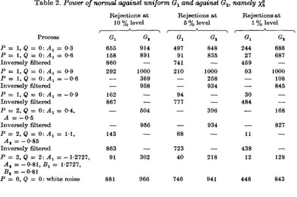
The Monte Carlo sample size is again N = 1000, with autoregressive-moving average process realizations of length n = 200 as in §2. Results are presented in Table 2. The estimated power of the independent case is given in the last row, power being the number of rejections x 10~3. Strong correlation leads to low power and the effect is more drastic

for high frequency correlation patterns. The rows 'inversely filtered' are explained below. If the distribution G of the input noise Zt is long-tailed, double exponential for example,

the loss of power is slightly less severe. Strong correlation patterns of high frequency type still lead to a reduction of power by up to a factor of 6. Details may be obtained from the author. For O asymmetric, the loss of power for low frequency correlation patterns is slight. For high frequency patterns it again becomes large. A remedy for this breakdown of power for model (1) is straightforward. I t improves at the same time the approximation to the distribution of the test statistic under the hypothesis:

(i) the parameters of the autoregressive-moving average process are estimated by one of the established identification methods (Box & Jenkins, 1970, Chapter 6);

(ii) with the estimated parameter vectors A and B we inversely filter the series Xt to

Zt so that it becomes approximately white noise, i.e. gives independent identically

dis-tributed values;

Ooodness-of-fit tests for correlated data

₆₆₇

This was done for some of the cases in Table 2. For step (i) the following approximate maximum likelihood estimates for normal autoregressive processes of order 1 and 2 were used, in spite of the nonnormality of the Zt:

order 1: Ar = &; order 2: Ax = px{l - -p{),

where pi is the estimate of autocorrelation of lag t. The determination of the order of

auto-regression is a separate problem; the true order was assumed. The results are in Table 2 in the rows' inversely filtered', for the process of the row above. There is a good improvement of power in all cases.

Table 2. Poioer of normal against uniform Ox and against Oit namely ^§

Process P = 1, Q = 0:A1 = 0-3 P = 1, Q = 0: A1 = 0-6 Inversely filtered P = 1, Q = O-.A} = 0-9 P = 1, Q = 0: At = - 0 - 6 Inversely filtered P = 1, Q = 0: Ax = - 0 - 9 Inversely filtered P = 2, 0 = 0: A1 = 0-4, 4 = - 0 - 5 Inversely filtered P = 2,Q = 0:A1 = 1 1 , At = -0-85 Inversely filtered P = 2, <3 = 2 : ^ ! =-1-2727, A, = - 0 - 8 1 , 5 ! = 1-2727, B, = - 0 - 8 1 P = 0, Q = 0: white noise Rejections at 10% GX 655 158 860 292 — 162 867 — 143 863 91 881 , level Gt 914 891 — 1000 369 958 — 604 956 — — 302 966 Rejections at 5 % level A G i 497 91 741 210 — 94 777 — — 68 723 40 746 848 835 — 1000 258 934 — — 396 934 — — 218 941 Rejections at 1 % <?! 244 27 459 93 — 30 484 — — 11 438 12 448 level A 688 687 — 1000 108 845 — — 168 827 — — 128 843

4. LIMITATIONS OF THE MODEL

Two types of deviations can jeopardize model (1) and as a consequence the inverse filtering procedure (i)—(iii). First, there may be a generation law of the type Zt -»- Xt with

Zt an independent stationary process, but the transformation may be nonlinear. A general

identification algorithm for nonlinear systems is not available. That any wide sense sta-tionary process with absolute continuous integrated spectrum can be linearly transformed to an uncorrelated process is of no help and may obscure the real problem. In many cases where a nonlinearity exists, it is, however, of small order and we can neglect it to a first approximation.

Secondly, a serious objection is the following: Xt may not have a representation of the

form Zt -> Xt with Zt white noise, and with the transformation invertible. This is for

568 THEO GASSEB

obvious that inverse filtering is then not feasible. It is more dangerous when this situation holds for a component St of Xt, the 'signal process', on which is superposed coloured or

white noise of a different kind. This occurs in E.E.G. analysis with Gaussian noise and a possibly non-Gaussian signal concentrated in some frequency bands. Inverse filtering would blow up the noise and pull down the signal, and a test in the Zt domain would indicate

normality even in cases of a non-Gaussian signal. This is the reason for considering model (2) in §5.

5. TEST FOE NORMALITY BY cruMxrLAi<rrs

As outlined in §1, E.E.G. analysts interested in testing their data for normality have mainly used the x% test, and in a few cases the Kolmogorov-Smirnov test. Neither is a

particularly good choice for the speoific hypothesis of normality (Shapiro, Wilk & Chen, 1968). There exist, however, powerful and at the same time simple tests for the particular case of the normal distribution. An attractive possibility is to use suitably normalized 3rd and 4th order cumulants. They are easy to evaluate, are location and scale invariant and have excellent power for a broad class of continuous alternatives. If we are confronted with the problem of correlated data, they have the additional advantage that they generalize quite easily. For a large sample {Xk: k = 1,..., n} from a stationary process Xt, 3rd and 4th

order sample cumulants are defined in the usual way, the difference between k statistics and sample cumulants being negligible. Then

k\ = n~lsA — 3n~2 Sgflj + 2n~2s\,

*j

= £

X{.

fc-i

The application of the test statistic in a large-sample situation is based on the following theorem.

THEOREM. Suppose that there is a Gaussian process{Xt} (t = 0, ± 1,...), E(Xt) = 0, vnth

covariance function Rk and spectrum F(v), with

£ I.RJ < 00.

fc-0

Then

(i) ni&a and nikt are asymptotically jointly normal toith expectation zero and finite variances

and covariances;

(ii) var(^8) = 6n-1 £ A : - - c o

£ i

, ^ ) = 0.

Assertion (i) can be proved by appealing to a mixing condition. For this situation, how-ever, a theorem by Sun (1965) is more specific. Some straightforward manipulations are needed to show the sufficiency of our condition. A complete proof of assertion (ii) would involve some tedious calculations, based on the decomposition of higher-order momenta into momenta of order two.

Goodness-of-fit tests for correlated data 569

The following assumptions are needed to characterize the properties of £, and iA for a

broad class of alternatives; lm denotes the mth order cumulant.

ASSUMPTIONS.Form = 2,3,...,(I) Zkl---Zkm_l\cm(k1>...,km_1)\ < oo,

(II) Sfcl."£*»-, \kMK->hn-l)\ < CO

withj = 1, ...,m-land cjl^, ....ft,^) = Jm( ^ o . ^ v •••<Xkm

-J-THBOBBM. Assume that Xk is a strictly stationary process, with finite, moments of arbitrary

order. Then

(A) given assumption I, £3 and fct are asymptotically unbiased and consistent estimates of

03(0,0) and c4(0,0,0);

(B) given assumption II, «g and kt are asymptotically jointly normally distributed.

Proof. For simplicity, assume E(Xk) = 0. Using stationarity we have, for F = E or I,

i n n 1 n - 1

This formula, together with the definition of cumulants in terms of moments and assump-tion I, leads to unbiasedness. For the proof of consistency we note that the assumpassump-tion I also holds for Yt = {Xi — X). By the fact that those partitions that are not indecomposable

cancel and by appealing to assumption I, we obtain consistency. The proof of (B) is most elegantly based on the asymptotic normality of linear estimates of 3rd and 4th order polyspectra (Brillinger & Rosenblatt, 1967).

Sample skewness and kurtosis are obtained by normalization:

COBOLLABY. The quantities nlfii and ni/?a ore asymptotically jointly normally distributed

vrith

k--a>

The simple proof of this corollary is omitted.

6. THE APPUCATTON OF fix AND y?a TO STATIONARY PBOCESSES

As in the independent case, the normal approximation can be safely used only for large sample size. A simple way to test the simultaneous hypothesis fix = 0, /?2 = 0 approximately

at a level a is to do the tests individually at levels \a. The first step consists in estimating ~Lp% and SpJ, by truncating to a finite lag and inserting correlation estimates. The choice of the truncation point should be guided by a careful analysis of the empirical correlation

570 T H B O G A S S E B

function and should be independent of n. The use of/^ and /?2 is suggested as a preliminary test statistic for model (2), where inverse filtering is impossible when the signal process has its energy concentrated in some frequency bands. The application to a broad class of E.E.G. samples revealed a frequent violation of the hypothesis of normality of the amplitude dis-tribution. Related to skewness andkurtosis are polyspectra which provide a test of normality not only of the first-order distribution of the stochastic process. The bispectrum for example is the spectral decomposition of the mixed third cumulant. For an application to E.E.G. data, see Dumermuth et al. (1971). Polyspectra have the additional advantage of being quite insensitive to violations of stationarity occurring in E.E.G. analysis. The need for large data size and relatively sophisticated mathematics may inhibit the widespread use of polyspectra.

REFERENCES

Box, G. E. P. & JENKINS, G. M. (1970). Time Series Analysis, Forecasting and Control. San Francisco: Holden Day.

BRUXINGKR, D. R. & ROSENBLATT, M. (1967). Asymptotic theory of estimates of fc-th order spectra. In Spectral Analysis of Time Series, Ed. B. Harris, pp. 153-88. New York: Wiley.

CHEBNOFF, H. & LEHMA^VN", E. L. (1954). The use of maximum likelihood estimates in %* tests for good-ness of fit. Ann. Math. Statist. 23, 579-86.

DUMEBMTJTH, G., HUBEB, P. J., KLETNEB, B. & GASSEB, T. (1971). Analysis of the interrelations between frequency bands of the EEG by means of the bispectrum. Electroenceph. Clin. Neurophysiol. 31, 137-48.

ELTJL, R. (1969). Gaussian behavior of the electroencephalogram during performance of mental task.

Science 164, 328-31.

KENDALL, M. G. & STUABT, A. (1967). Advanced Theory of Statistics, Vol. 2. London: Griffin. MALLOWS, C. L. (1967). Linear processes are nearly Gaussian. J. Appl. Prob. 4, 313-29.

PATANAKAB, V. N. (1954). The goodness of fit of frequency distributions obtained from stochastic processes. Biometrika 41, 450-62.

SAUNDEBS, M. G. (1963). Amplitude probability density studies on alpha and alpha-like patterns.

Electroenceph. Clin. Neurophysiol. 15, 761-7.

SHAPTBO, S. S., WILK, M. B. & CHEN, H. J. (1968). Comparative study of various tests for normality.

J. Am. Statist. Assoc. 63, 1343-72.

SUN, T. C. (1965). Some further results on central Emit theorems for non-linear functions of a normal process. J. Math, dk Mech. 14, 71-85.

WEISS, M. S. (1973). Non-Gaussian properties of the E.E.G. during sleep. Electroenceph. Clin.

Neuro-physiol. 34, 200-2.