Predictive Model for Strawberry Bud Weevil (Coleoptera: Curculionidae) Adults in Strawberry Fields

Predictive Model for Strawberry Bud Weevil

(Coleoptera: Curculionidae) Adults in Strawberry Fields

N. J. BOSTANIAN,1_{M. BINNS,}2_{J. KOVACH,}3_{G. RACETTE,}1_{ANDG. MAILLOUX}4

Environ. Entomol. 28(3): 398Ð406 (1999)

ABSTRACT Three different sampling methods (sweep net, D-Vac, tapping into a carton

con-tainer) were evaluated for Anthonomus signatus Say in strawberry Þelds. The results suggest that sampling with a sweep net reßects population numbers best. A predictive model for adult abundance was developed to describe and predict population build-up. The strawberry Þelds used in the study were in their 2nd yr of production. Overwintering adults generally begin to appear in a strawberry Þeld '300 cumulatitive degree-days (DD) calculated from 1 April at temperatures above 08C. These weevils attain maximum abundance anywhere from 500 to 670 DD. Within that interval, a treatment with cypermethrin or chlorpyriphos was effective against this pest. The summer generation attained maximum abundance anywhere from 1,250 to 1,650 DD. A treatment with chlorpyriphos at 1,679 DD reduced the summer generation of weevils and decreased clipped buds in the Þeld the following year.

KEY WORDS Anthonomus signatus, predictive model, adult abundance, management

THE STRAWBERRY BUDweevil, Anthonomus signatus Say, is 1 of 2 key insect pests of strawberries in Northeast-ern North America. The other is the tarnished plant bug, Lygus lineolaris (Palisot du Beauvois). Overwin-tering weevils have been reported on strawberries from mid-May to the end of June with maximum abun-dance toward the end of May in Quebec (Rivard et al. 1979). In New York, these events occur '2 wk earlier (Kovach et al. 1993).

Decreases in yield can be dramatic depending on cultivar. Losses in Quebec range from 10 to 70% (Para-dis 1979). In New York, strawberry yield reductions range from 50 to 100% (Schaefers 1978). Early matur-ing cultivars are more susceptible to injury than late maturing cultivars (Dorval 1938). The biology of this insect was described by Mailloux and Bostanian (1993). They conÞrmed earlier observations that the insect had 4 distinct nonoverlapping stages of devel-opment (egg, larva, pupa, adult) (Clarke and Howitt 1975). Furthermore, Mailloux and Bostanian (1993) showed that a 1:1 sex ratio was prevalent throughout spring and summer. The maximum abundance of each developmental stage was determined in relation to cumulative degree-days (DD). Currrently, monitor-ing is carried out very early in the sprmonitor-ing by countmonitor-ing the number of cut buds per ßower cluster per linear meter and comparing this with a tentative action threshold of 2 clipped buds per meter (Kovach et al.

1993), although some recent work suggests that this threshold is too low (Pritts et al. 1999). However, as weevil populations increase from zero to threatening numbers within a very short period (Mailloux and Bostanian 1993), management action based on dam-age alone risks being very late. Because there is no generally accepted sampling technique and the timing of control measures is difÞcult, many growers make a prophylactic treatment at the onset of buds, to be followed by a 2nd prophylactic treatment just before bloom.

This study was used to evaluate 3 different sampling techniques to estimate the abundance of this insect. Abundance data were collected to develop a predic-tive model (based on degree-days) to estimate when adult beetles would Þrst be seen and when peak abun-dance could be expected to occur. Management con-trol based on the results was then validated using data collected in Quebec and New York during 1994.

Materials and Methods

Model Development. Field observations were made

twice a week from early May to the end of August in 1976 and 1987Ð1991 in strawberry Þelds not treated with insecticides. The Þelds were in their 2nd yr of production and their sizes ranged from 0.5 to 0.75 ha. They were situated at LÕAssomption, Frelighsburg, Lavaltrie (near Montreal), St. Louis de Terrebonne, and St. Augustin (near Quebec city). They represent the major strawberry-growing regions of Quebec.

Eighteen sets of data on strawberries (15 on ÔRed-coatÕ and 3 on ÔBountyÕ) were collected over a period of 15 yr from the above mentioned locations (Table 1). Counts were made by walking a W-shaped pattern across the Þeld and collecting samples. The following

1_{Horticulture Research and Development Centre, Agriculture and} Agri-Food Canada, Saint-Jean-sur-Richelieu, QC, Canada J3B 3E6.

2_{Eastern Cereal & Oilseed Research Centre, Agriculture and} Agri-Food Canada, Ottawa, ON, Canada K2C 1Y2.

3_{New York State Agriculture Experiment Station, Cornell} Univer-sity, Geneva, NY 14456Ð0462.

4_{Institut de Recherches et de De´veloppement, en} Agro-Environ-nement, Saint-Hyacinthe, QC, Canada J2S 480.

3 sampling techniques were used: (1) 200 suctions with a D-Vac insect aspirator (D-Vac, Riverside, CA). (2) Two hundred sweeps with a 71 cm long heavy duty muslin insect net. That was D-shaped and had a 38 cm diameter. (3) Tapping 100 ßower clusters twice each over a carton container (500 ml capacity and 10 cm

diameter); the number of weevils present was re-corded and the weevils were allowed to escape.

No samples were recorded from the edges of the Þelds, and all sampling was done between 10.00 and 13.00 hours on sunny days. In 2 of the sets, replicate sets of 100 container tappings were taken to assess

Fig. 1. Data from the 3 sampling techniques (C, container tapping; N, sweep net; D, D-Vac).

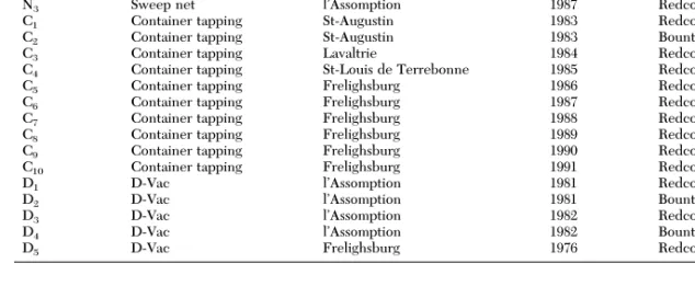
Table 1. Methods, cultivar, and year used to collect data in Quebec, Canada

Series Method Location Year Cultivar _{sample units}No. of N1 Sweep net lÕAssomption 1985 Redcoat 42

N2 Sweep net lÕAssomption 1986 Redcoat 22

N3 Sweep net lÕAssomption 1987 Redcoat 20

C1 Container tapping St-Augustin 1983 Redcoat 24

C2 Container tapping St-Augustin 1983 Bounty 24

C3 Container tapping Lavaltrie 1984 Redcoat 24

C4 Container tapping St-Louis de Terrebonne 1985 Redcoat 24

C5 Container tapping Frelighsburg 1986 Redcoat 19

C6 Container tapping Frelighsburg 1987 Redcoat 21

C7 Container tapping Frelighsburg 1988 Redcoat 24

C8 Container tapping Frelighsburg 1989 Redcoat 32

C9 Container tapping Frelighsburg 1990 Redcoat 25

C10 Container tapping Frelighsburg 1991 Redcoat 38

D1 D-Vac lÕAssomption 1981 Redcoat 34

D2 D-Vac lÕAssomption 1981 Bounty 33

D3 D-Vac lÕAssomption 1982 Redcoat 41

D4 D-Vac lÕAssomption 1982 Bounty 41

sampling variability. Table 1 summarizes the location, year, cultivar, and number of samples per plot. A sample refers to 200 suctions (D-Vac), 200 sweeps (net sam-pling), or 100 tappings (tapping into carton containers). Ambient air temperature data were obtained from Environment Canada weather stations located ,8 km away from each strawberry Þeld. Cumulative degree-days above 08C from 1 April to the end of August were calculated using the Baskerville and Emin (1969) method.

Various preliminary attempts were made to relate the seasonal abundance data to temperature and pre-cipitation, but temperature was clearly the factor in-ßuencing development. The relationship between sample counts and degree-days was initially estimated by smoothing the data (Gaussian kernal method) us-ing Mathcad (Mathsoft 1995) separately for each sam-ple method (container, net, D-Vac). The results in-dicated so much variability within each method (Fig. 1) that Þtting an overall model was deemed

inappro-priate except possibly for net sampling. Therefore, the model was Þtted to each series of data separately and also to all net samples together.

Numerous abundance models have been suggested for variability of agricultural pest populations through-out the season based on thermal summation units (Niemczyk et al. 1992, CockÞeld et al. 1994). We chose to adapt models intended for estimating life histories (Kempton 1979, summarized in Manly 1990). The ad-aptation was to reduce the model from predicting all life stages to predicting only the adult stage. The der-ivation of the model for N(t), the total number of adults found at time t, follows. Because the data were totals of a large number of suctions, sweeps, or tap-pings, a Poisson distribution for N(t) was assumed. The goodness-of-Þt of the model was assessed by the residual deviance (McCullagh and Nelder 1989). The deviance is comparable to the residual error sum of squares in linear regression, but is dimensionless; if everything Þts well, the mean deviance (comparable

Fig. 2. Fitted curves for 3 net tapping series: N1, N2, and N3. Square brackets in N1and N2indicate 1st and 3rd quartiles

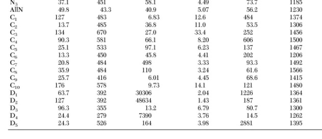
of the distribution of spring emergence from cages (Mailloux and Bostanian 1993). Table 2. Fitted parameters of the abundance model

Series M1 m1 g1 ₍₃₁₀u13₎ M2 m2 g2 ₍₃₁₀u23₎ N1 69.2 429 28.1 5.67 73.7 1197 218 5.53 N2 65.5 428 58.9 6.31 257 1467 407 96.9 N3 37.1 451 58.1 4.49 73.7 1185 661 7.62 AllN 49.8 43.3 40.9 5.07 56.2 1230 213 6.50 C1 127 483 6.83 12.6 484 1374 405 9.04 C2 13.7 485 36.8 11.0 53.5 1306 871 9.79 C3 134 670 27.0 33.4 252 1456 152 58.8 C4 90.3 581 66.1 8.20 606 1500 560 84.3 C5 25.1 533 97.1 6.23 137 1467 219 75.2 C6 13.3 450 45.8 4.41 202 1206 119 21.0 C7 20.8 484 498 3.33 93.3 1492 47556 11.9 C8 35.9 484 110 3.24 61.6 1566 811 5.74 C9 25.7 416 6.01 4.45 68.6 1415 7374 8.56 C10 176 578 9.73 14.1 121 1480 118 30.8 D1 63.7 392 30306 2.04 1226 1364 234 32.0 D2 127 392 48634 1.43 187 1361 3130 7.77 D3 96.3 355 13.2 6.79 80.7 1300 3594 6.99 D4 24.4 279 7390 3.76 14.5 1262 4913 2.73 D5 24.3 526 164 3.98 2881 1395 434 234

to the error mean square) should be equal to 1, and the deviance can be tested asx2_{. For the 2 datasets where} extra data had been collected (Table 1: C7, C10), a within-date residual deviance was also calculated for comparison. Genstat (1996) was used for all these calculations.

Data for spring emergence of adults from cages reported in Mailloux & Bostanian (1993) were col-lected during the same time and at the same location as 4 of the datasets. The data from the emergence cages were compared with the Þtted model (based on sample data) around the time of spring emergence to check for consistency.

Derivation of the Abundance Model. The basic

life-stage model suggested by Kempton (1979) takes the following form: the probability that an individual is in stage j at time t (i.e., is at that stage, in the Þeld and able to be sampled) can be written as the product of the following: (1) the probability that at time t it has matured to but not passed stage j, and (2) the prob-ability that it has not died in the meantime. Because we

are interested only in the adults, “stage j” is the emerg-ing adult, so we rewrite (1) above as follows: (1a) the probability that it has emerged by time t.

Two mathematical formulations of this have been mentioned in the literature. In one, the possibility of dying is deemed to begin when the “experiment be-gins,” which here would be 1 April when degree-days 5 0 (Manly 1990, p. 60). In the other, the pos-sibility of dying is deemed to begin when the “individual emerges,” which would be after 1 April (Manly 1990, p. 52). Although, in several instances including the version used here, there is no formal difference between the representations, we chose the 2nd as being more appropriate for the weevil data. Thus, an appropriate model has an emergence distri-bution, deÞned by the probability density f(x):

Probability that an individual emerges at time x, along with a survival distribution, deÞned by the prob-ability density w(t 2 x),

Probability that an individual survives from time x to time t 5 w(t 2 x).

Thus, the probability of emerging at time x and then surviving for a further time (t-x) can be written as f(x)

Table 3. Estimates in cumulative degree days (DD) for the 1st adult emergence in spring and maximum abundance of summer generation

Series _emergenceDD for 1 _{spring peak}DD at _{summer peak}DD at

N1 274 508 1282

N2 325 487 1471

N3 346 530 1244

Mean 315 508 1332

Standard error 37 22 122

All sweep net data 307 511 1311

C1 158 484 1438 C2 385 537 1356 C3 422 672 1463 C4 434 645 1509 C5 441 601 1475 C6 360 535 1238 C7 502 587 1508 C8 404 566 1639 C9 229 486 1488 C10 237 663 1523 Mean 357 578 1464 Standard error 111 68 107 D1 338 460 1388 D2 338 463 1403 D3 171 426 1341 D4 224 296 1393 D5 453 599 1393 Mean 305 449 1384 Standard error 110 108 24

Table 4. Control of the strawberry bud weevil on strawberry, 1994

Spring treatment Summer treatment

Frelighsburg Geneva Geneva

No. of berries Injured,_% a No. of berries Injured,_% b No. of berries Injured,_% c No. of berries Injured,_% d

Treated 627 0.5 538 2.2 695 0.9 695 1.6

Control 691 9.1 545 13.2 695 5.6 695 5.6

a_{10 d after treatment (Ripcord 400 EC applied on 3 July 1994 [549 DD] at 188 ml/ha).} b_{26 d after treatment (Ripcord 400 EC applied on 3 July 1994 [549 DD] at 188 ml/ha).} c_{17 d after treatment (Lorsban 4 E applied on 27 May 1994 [566 DD] at 2,336 ml/ha).} d_{1 yr after treatment (Lorsban 4 E applied on 22 July 1993 [1679 DD] at 2,356 ml/ha).}

Table 5. Deviance goodness-of-fit values for the overall model, and within-date error deviance values where data were available

Series

Overall Within date

Residual

deviancea df _devianceMeanb _devianceResidual df _devianceMean

N1 73* 34 2.2 N2 23 14 1.7 N3 18 12 1.5 C1 106* 16 6.7 C2 15 16 0.9 C3 33* 16 2.1 C4 75* 16 4.7 C5 20* 11 1.8 C6 19 13 1.5 C7 32* 16 2.0 40* 6 6.7 C8 110* 24 4.6 C9 51* 17 3.0 C10 148* 30 4.9 21 14 1.5 D1 159* 26 6.1 D2 166* 25 6.6 D3 163* 33 4.9 D4 218* 33 6.6 D5 77* 24 3.2

*_{, SigniÞcant (P , 0.05) departure from Poisson.} a_{To be tested as chi square (deviance is dimensionless).} b_{Residual deviance divided by degrees of freedom.}

3 w (t 2 x). When this formula is integrated over values of x less than or equal to t, the probability of having emerged and still being alive at time t can therefore be written as

p~t! 5

E

f~x! w~t 2 x! dx.

This formulation was used for both spring and sum-mer generations. Esum-mergence for the 1st generation refers to emergence from winter diapause, and for the summer generation it refers to emergence from the pupa. Of course, the parameters of the probability density functions are different for spring and for sum-mer.

Several distributions have been proposed for f(x) (e.g., gamma, Gaussian, inverse Gaussian). For the bud weevil, the Gaussian distribution was rejected because it is symmetric. Both gamma and inverse Gaussian were tried, but f(x) represented by the gamma distribution was found to Þt the data better. Like Manly (1990, p. 50) we used w(t) 5 exp(-ut). Thus, the formula for p(t) is

p~t! 5

E

g~m, g, x! exp(2u@t 2 x#) dx, [1]

where g(m, u, x) is the gamma probability distribution function with meanm and exponent g:

g~m,g,x! 5

S

D

The expression for p(t) in equation 1 can be repa-rameterized so that the formula for emergence and mortality are mathematically separate.

p~t! 5

E

S

D

S

D

E

However, for much of the bud weevil data, this formula (equation 2) cannot be used numerically be-cause the emergence probability factor [the integral of g(m,g, x)] is often very small, whereas the other

Fig. 3. Fitted curves for 6 container tapping series, C1ÐC6. Square brackets in C5and C6indicate 1st and 3rd quartiles

factor is very large, causing unacceptable round-off errors. Therefore, the complete integral of equation 1 had to be approximated by numerical quadrature. Us-ing a 3-point Simpson rule (Abramowitz and Stegun 1972) for each interval between sampling times gave poor precision, especially at the beginning of the sea-son, so the season was divided into 50 intervals, the function estimated by 3-point Simpson rules in each, and interpolated at the sample times.

Based on the above formulation, 1st- (i 5 1) and 2nd- (i 5 2) generation adults were modeled using the same basic formulae, but with different parameters:

p~t,mi,gi,ui! 5

E

g~mi,gi, x! exp~ 2ui@t 2 x#! dx [3]

and the complete model for N(t), the total number found at time t, is a weighted sum of these.

N~t! 5 M1p~t,m1,g1,u1! 1 M2p~t,m2,g2,u2! [4] The parameters to be Þtted are as follows:mi5 mean of the emergence distribution in generation i,gi5 exponent parameter of the emergence distribution for

generation i,ui5 mortality parameter for generation i, Mi5 constants, 1 for each generation.

Model Validation. The individual Þtted models

were used to estimate key pest management indicators of abundance: time (degree-days) of appearance of 1 adult in spring, time of peak spring abundance, and time of peak summer abundance. In 1994, 2 of these indicators (peak spring and summer abundance) were evaluated in Frelighsburg, Quebec, and Geneva, NY. A 3-yr-old (2nd yr of production) cultivar ÔGlooscapÕ strawberry plot was used in Quebec and a similar but slightly larger plot containing ÔEarliglowÕ, ÔAllstarÕ, and ÔHoneoyeÕ was used in New York. At each location, the plots were divided such that one half was treated according to the model, and the other half was left untreated as a control. At both locations, the control plots received no insecticide treatments for this or any other pest. For the treated plots at Frelighsburg, cypermethrin (Ripcord 400 EC[emulsiÞable concen-trate] [American Cyanamid, Wayne, NJ]) was ap-plied to 0.05 ha at 188 ml/ha when 549 DD had been accumulated and berry clusters were examined twice. The 1st observation was 10 d after treatment and the 2nd was at harvest. At Geneva, chlorpyriphos (Lors-ban 4 E [emulsiÞable] [Dow-Elanco, Indianapolis, IN]) was applied to 0.09 ha at 2,336 ml/ha, when 566 DD (27 May) had been accumulated. One hundred

berry clusters from each plot were examined for clipped berries at 4 different times (31 May, 2 June, 7 June, and 13 June). Moreover, a summer treatment, at 1,679 DD on 22 July 1993, was also carried out in New York against the summer adults before they entered into reproductive diapause and disappeared on or into the soil. The following year, berries from this treated Þeld were compared with berries from an adjacent control plot.

Results

The Þtted parameters of the abundance model are shown in Table 2. The Þtted curves are presented in Figs. 2Ð5. The lower and upper quartiles of the distri-bution of spring emergence in cages (Mailloux and Bostanian 1993) are plotted in the Þgures for N1, N2, C5, and C6.

Lower

quartile, DD Median,DD quartile, DDUpper

N1 286 320 419

N2 367 375 390

C5 411 454 581

C6 375 398 509

Estimated times for Þnding the 1st spring adult and for spring and summer peaks are shown in Table 3. The

expected time in spring for Þnding the 1st emerging adult (using any one of the 3 sampling techniques) was found to be between 300 and 350 DD, although with anything but sweep net the variability was high. Ex-pected time for spring peak ranged from around 450 DD (D-Vac), 510 DD (sweep net) to 580 DD (con-tainer tapping), with high variability except with sweep net. Expected time for the summer peak ranged from around 1,310 DD (sweep net), 1,380 DD (D-Vac) to 1,460 DD (container tapping), with high vari-ability except for D-Vac.

Results from the 2 Þeld evaluations are presented in Table 4. With a spring treatment in Geneva, 0.9% of the buds were clipped in the treated plot, 17 d after treat-ment, compared with 5.6% in the untreated control plot. At Frelighsburg, the percentages of clipped ber-ries were 0.5% in the treated plot and 9.1% in the untreated control plot 10 d after treatment. At harvest time these percentages increased to 2.2 and 13.2%, respectively. In the summer treated plot (1,679 DD), 1.3% of the berries were clipped, the following year in Geneva, whereas, in the control plot the percentage of clipped berries was 5.6%.

Discussion

Fitting the Model. Sample estimates of population

sizes varied considerably among the series of data. Maximum values for 100 container tappings ranged from ,10 (C2) to .60 (C4) among spring generation data, and from ,10 (C5) to around 200 (C1) among summer generation data. In some datasets the peak spring generation densities were much larger than the summer ones (e.g., N2), in some they were similar (e.g., C4, C8), and in others the peak summer densities were much larger (e.g., C1, C2). It is not surprising therefore that the Þtted parameter values varied greatly from one dataset to another.

The 2nd-generation data seemed to Þt the model better than the 1st-generation data (Figs. 2Ð5). In the spring, the distribution is likely to be more patchy than in the summer because of adults emerging not only from the strawberry Þeld but also from surrounding Þelds and brush. There was much variability in the data: samples taken only a few degree-days apart from each other occasionally provided greatly differing es-timates of abundance, which could not be accounted for by any reasonable model (for example, D2 be-tween 500 and 900 DD, and C5around 1,500 DD). This variabilty is reßected in the goodness-of-Þt tests for the models (Table 5). The D-Vac data appear to be especially variable. The sweep net data Þtted better than the container tapping data, but the larger number of net sweeps (200) than container tappings (100) may account for that. In 2 of the datasets where con-tainer tapping was used, it was possible to estimate “within date” variability (Table 5). Comparison with the Poisson model indicated large heterogeneous vari-abilty among samples. Heterogeneity beyond that ex-pected from a Poisson distribution may have contrib-uted to the variability of data points around the curves as, for example in C4, C7ÐC10.

In most sampling situations, the mean count from a sample consisting of 100 sampling units would have relatively small variance, and would be a good pre-dictor of actual abundance. The fact that there was heterogeneity above the Poisson level implies that the variability among individual counts was extremely large. In general, variability was least for net sampling, higher for container sampling, and very high for D-Vac sampling (Table 5). It is possible that D-Vac sampling, holding the apparatus just above the plant canopy, is harder to perform consistently. For this reason, we paid less attention to the D-Vac results.

Future work on estimating density of Anthonomus sp. would need to consider these and other compli-cations. For example, A. pomorum displayed predom-inantly nocturnal behavior patterns in both laboratory and Þeld studies (Duan et al. 1996). Therefore, for such species, the numbers of individuals that can be sampled on the plants during the day may not repre-sent a constant proportion of the true population, thus increasing sample variability.

Pest Management. For the cultivars examined here,

harvest takes place approximately between 950 and 1,500 DD (Mailloux and Bostanian 1991), so the bud weevil affects harvest only through its 1st generation. Figs. 2Ð5 and Table 3 show that the spring generation attains maximum abundance anywhere from 500 to 670 DD above 08C.

The results in Table 4 suggest that control measures based on degree-days can be effective in maintaining weevil populations at low numbers and thus reduce berry loss. A summer treatment after harvest is an interesting concept and the results shown here look promising but further research needs to be done. If such a pest management program becomes viable, it means that no pesticides would be needed against this pest before the berries are picked, and several insec-ticides that cannot be used currently because of res-idue considerations could then be used without much concern, because these would be applied a year before harvest.

A pesticide intervention may not always be neces-sary, especially in the 1st yr of harvest. However, for the 2nd yr of harvest, the results of this study indicate that the optimal time of chemical treatment to control the strawberry bud weevil is between 500 and 670 DD above 08C calculated from 1 April. The beetles may be sampled either by sweeping or tapping into carton box of 500-ml capacity. The percentage of clipped buds after treatment carried out in that interval of time would be commercially acceptable to growers. Un-fortunately, a relationship between weevil numbers and clipped buds (harvest loss) does not exist. Such a relationship is a prerequisite for establishing an action threshold based on pest abundance and a sampling program.

Acknowledgments

Agriculture and Agri-Food Canada Contribution No. is 335/99.04.21R at The Horticulture Research and Develop-ment Center, St. Jean-sur-Richelieu, QC, Canada.

References Cited

Abramowitz, M., and I. A. Stegun. 1972. Handbook of

math-ematical functions. U.S. Department of Commerce, Na-tional Bureau of Standards, Washington, DC.

Baskerville, G. L., and P. Emin. 1969. Rapid estimation of

heat accumulation from maximum and minimum tem-perature. Ecology 50: 514Ð517.

Cockfield, S. D., S. M. Fitzpatrick, K. V. Giles, and D. L. Mahr. 1994. Hatch of blackheaded Þreworm (Lepidoptera:

Tortricidae) eggs and prediction with temperature-driven models. Environ. Entomol. 23: 101Ð107.

Clarke, R. G., and A. J. Howitt. 1975. Development of the

strawberry weevil under laboratory and Þeld conditions. Ann. Entomol. Soc. Am. 68: 715Ð718.

Dorval, P. 1938. Les ennemis du fraisier. Rev. Oka 12: 1Ð10. Duan, J. J., D. C. Weber, B. Hirs, and S. Dorn. 1996. Spring

behavioral patterns of the apple blossom weevil. Entomol. Exp. Appl. 79: 9Ð17.

Genstat. 1996. Genstat for Windows. NAG, Oxford, UK. Kempton, R. A. 1979. Statistical analysis of frequency data

obtained from sampling an insect population grouped by stages, pp. 401Ð418. In J. K. Ord, G. P. Patil, and C. Taillie [eds.], Statistical distributions in scientiÞc work. Inter-national Cooperative, Burtonsville, MD.

Kovach, J., W. Wilcox, A. Agnello, and M. Pritts. 1993.

Strawberry IPM scouting procedures: a guide to sampling for common pests in New York State. IPM No. 203b. Cornell Cooperative Extension, Cornell University, Ithaca, NY.

Mailloux, G., and N. J. Bostanian. 1991. The phenological

development of strawberry plants and its relation to tar-nished plant bug seasonal abundance. Adv. Strawberry Prod. 10: 30Ð36.

1993. Development of the strawberry bud weevil

(Co-leoptera: Curculionidae) in strawberry Þelds. Ann. En-tomol. Soc. Am. 86: 384Ð393.

Manly, B.F.J. 1990. Stage Structured populations, sampling,

analysis and simulation. Chapman & Hall, London.

Mathsoft. 1995. Mathcad PLUS 6.0. Mathsoft, Cambridge,

MA.

McCullagh, P., and J. A. Nelder. 1989. Generalized linear

models, 2nd ed. Chapman & Hall, London.

Niemczyk, H. D., R.A.J. Taylor, M. P. Tolley, and K. T. Power. 1992. Physiological time-driven model for predicting frst

generation of the hairy chinch bug (Hemiptera: Lygaei-dae) on turfgrass in Ohio. J. Econ. Entomol. 85: 821Ð829.

Paradis, R. O. 1979. Essais dÕinsecticides contre lÕanthonome

du fraisier, Anthonomus signatus Say, pre´sent conjointe-ment avec la punaise terne, Lygus lineolaris (P. de B.) dans des fraisie`res. Phytoprotection 60: 31Ð40.

Pritts, M., M. J. Kelly, and G. English-Loeb. 1999.

Straw-berry cultivars compensate for simulated bud weevil (An-thonomus signatusSay) damage in matted row plantings. Hort. Sci. 34: 109Ð111.

Rivard, I., G. Mailloux, R. O. Paradis, and G. Boivin. 1979.

Apparition des adultes de lÕanthonome du fraisier, An-thonomus signatusSay, en fraisie´res et framboisie´res au Que´bec. Phytoprotection 60: 41Ð46.

Schaefers, G. A. 1978. EfÞcacy of Lorsban brand

insecti-cides for the reduction of strawberry “bud” weevil, An-thonomus signatus Say, damage in stawberries. Down Earth 35: 1Ð3.

Received for publication 8 April 1998; accepted 9 February 1999.