POISSON RISK MODEL: DIVIDENDS
BY
HANSJÖRG ALBRECHER, ERIC C.K. CHEUNGAND STEFAN THONHAUSER
ABSTRACT
In the framework of the classical compound Poisson process in collective risk theory, we study a modifi cation of the horizontal dividend barrier strategy by introducing random observation times at which dividends can be paid and ruin can be observed. This model contains both the continuous-time and the discrete-time risk model as a limit and represents a certain type of bridge between them which still enables the explicit calculation of moments of total discounted dividend payments until ruin. Numerical illustrations for several sets of parameters are given and the effect of random observation times on the performance of the dividend strategy is studied.
KEYWORDS
Compound Poisson risk model; horizontal dividend barrier strategy; Erlangi-zation.
1. INTRODUCTION
In the classical compound Poisson risk model, the surplus process {C(t)}t $ 0 of an insurance company is described by
i (t = (t) ) Y, 0, C x ct S x ct t ( ) i N t 1 $ + - = + -= :
/
(1)where x = C(0) $ 0 is the initial surplus level, {S(t)}t $ 0 is the aggregate claims process and c > E[S(1)] is the (constant) premium income per unit time. More specifi cally, {N(t)}t $ 0 is assumed to be a homogeneous Poisson process with rate l > 0, and the claim sizes Y1, Y2, … form a sequence of independent and identically distributed (i.i.d.) positive random variables (r.v.’s), independent of {N(t)}t $ 0, and with generic continuous r.v. Y, c.d.f. FY(·), p.d.f. fY(·) and Laplace transform fY(·). If C(t) < 0 for some t > 0, then this event is called
ruin of the risk process (see e.g. Asmussen & Albrecher [4] for a recent survey of risk models).
Under the horizontal dividend barrier strategy, any excess of the surplus over a pre-defi ned barrier level b $ 0 is immediately paid out as dividends to the shareholders of the company as long as ruin has not yet occurred for this modifi ed process. The effect of this strategy on the risk process and on the resulting total discounted dividend payments (where the discount rate is usu-ally assumed to be a constant d $ 0) is extensively studied in the literature.
In particular, it turns out that in certain situations the above model assump-tions lead to pleasant and explicit expressions for some quantities of interest, such as the moments of the total discounted dividend payments until ruin (see for instance Dickson & Waters [7] and Gerber & Shiu [9]).
However, in a continuous-time model the horizontal dividend strategy implies a continuous dividend payment stream whenever the surplus process is at level b. In practice, it is more reasonable for the board of the company to check the balance on a periodic basis and then decide whether to pay dividends to the shareholders, resulting in lump sum dividend payments at such discrete time points rather than continuous payment streams. This line of reasoning leads to the study of the horizontal dividend strategy in discrete-time risk models (cf. e.g. Dickson & Waters [7]). But the latter models have the draw-back of leading to a (often large) system of linear equations for the quantities of interest. Consequently, this approach usually does not lead to explicit solutions and it is then diffi cult to gain structural insight in the infl uence of parameters and to identify optimal choices, such as the optimal barrier level.
In this paper, we want to pursue the idea of only acting at discrete points in time, but at the same time maintaining some of the transparency and elegance of the time approach. For that purpose we consider the continuous-time compound Poisson risk model (1), but ‘look’ at the process only at ran-dom times {Zk}3k = 0 (called observation times) with Z0 = 0, at which a lump sum dividend payment of size x – b will take place if the current surplus level
x exceeds the barrier level b, and the process will be declared ruined if x < 0.
Note in particular that ruin can now only be observed at these random obser-vation times and so a surplus level below 0 between obserobser-vation points will only result in actual ruin if it is also negative at the next observation time. The randomness of observation times will allow to carry over some of the prop-erties of the classical continuous-time observation to this discretized version; in particular, {C(Zk)}k $ 1 can be interpreted as a ‘new’ random walk.
Let Tk = Zk – Zk – 1 (k = 1, 2, …) be the k-th time interval between observa-tions, and assume that k=1
3 k
{T } is an i.i.d. sequence distributed as a generic r.v. T and independent of {N(t)}t $ 0 and 1.
3 i = i
{Y } With the above-defi ned div-idend rule with barrier b, denote the sequences of surplus levels at the time points {Z }k- 3k =1 and k=1 3 k {Z } by k=1 3 b( {U k)} and k=1 3 b( {W k)} respectively, i.e., k=1 3 b( {U k }) and k=1 3 b(
{W k)} are the surplus levels at the k-th observation
before (after, respectively) potential dividends are paid. With initial surplus
FIGURE 1: Sample path of a compound Poisson risk model under randomized observations. ( S(Z ) ( (k) b ) -[ ( ) ] k) { (k), }, , , . min W k T S Z W b k 1 1 2 b k k k 1 b b f = - + - = = -c , U U
The time of ruin is defi ned by tb = Zkb, where kb = inf{k $ 1 : Wb(k) < 0} is the
number of observation intervals before ruin. A sample path under the present model is depicted in Figure 1.
For mathematical tractability, we will assume that the r.v. T is Erlang(n) distributed with density
gt = (t t ) 1 -) ( ! 0 fT e t > -gn n-1 : n ,
and corresponding Laplace transform fT(s) =
#
03e-stf tT( )dt=^g+gshn, where g > 0 is the rate parameter. Note that n = 1 refers to exponentially distributedobservation intervals (which due to the lack-of-memory property of the expo-nential distribution refl ects the case where the time until the next observation (dividend/ruin decision) does not depend on the time elapsed since the last decision).
For any fi xed n, the r.v. T converges in distribution to a point mass at 0 for
g " 3, so this limit corresponds to the classical continuous-time risk model with horizontal barrier strategy with barrier at b (i.e. continuous observation of the process and hence continuous decisions on dividends and ruin).
On the other hand, if one fi xes E[T ] = h and chooses n suffi ciently large, this approximates the discrete-time risk model with time step h (i.e. determin-istic observation intervals h), since the Erlang distribution for n " 3 and fi xed expected value E[T ] = h converges in distribution to a point mass in h.
This so-called Erlangization technique and its computational advantages were exploited for other purposes (in particular for randomizing a fi nite time hori-zon for ruin problems) by Asmussen et al. [5] (see also Ramaswami et al. [13] and Stanford et al. [16, 17]). For statistical inference for continuous-time risk processes with deterministic discrete observation times, see Shimizu [15].
In the companion paper Albrecher et al. [1], we will investigate the expected discounted penalty function (Gerber & Shiu [9]) under random observation times. In the present paper we study the effect of the randomized observation times on the moments of the total discounted dividend payments until ruin for a discount rate d $ 0. Let
(0)=x, Z d -( b b = , (x b) e k) + W x R M k k b 1 k b ! D -= d ; :
/
7U A . (2)With time 0 an intervention time, the total discounted dividend payments until ruin are represented by the r.v.
= , , d d ( ; ) 0, ( ; ), 0 , ( ), . x b x x b x b b b x b < > M M # # D D D - + d 0, ; x b : Z [ \ ] ] ] ]
In particular, the distribution of DM, d (x; b) for 0 # x # b already determines Dd (x; b) for arbitrary x.
Denote the m-th moment of Dd (x; b) by
,
m d(x; ) = E (x; ) 0, 1, 2, ,
V b Dd b m= f
m
: 9^ h C, (3)
which is the main quantity of interest in this paper. We adopt the usual con-vention that V0, d (x; b) / 1 and shall use the abbreviation V(x; b) := V1, d(x; b). The quantities (3) have been studied for the classical compound Poisson model with continuous observation in Dickson & Waters [7].
We present three different approaches to study Vm, d (x; b) for randomized observation intervals. In Section 2 we start with adapting the generator approach to the present model. If T is exponentially distributed, this leads to a system of integro-differential equations (IDEs) defi ned on different surplus layers that are connected by certain contact conditions (the resulting analysis has similarities with equations that appear in multi-layer dividend policies of the classical model, see Albrecher & Hartinger [3] and Lin & Sendova [12]). This approach is par-ticularly instructive when analyzing conditions for the optimality of the dividend barrier in this model (see Section 5). In Section 3 the so-called discounted density of increment will be used to derive integral equations for Vm, d (x; b) which are more tractable for a large class of claim and inter-observation time
distributions. This is important in the Erlangization procedure because we would like to increase n gradually in the approximation. As a third alternative, in Section 4 the discounted density of overshoot is used for the analysis. This will lead to a factorization formula which is of independent interest and plays an important role in Section 4.1 when certain classical formulas are generalized. Section 6 gives numerical illustrations that underline the computational advan-tages of the method for approximating the discrete-time model. More over, the effect of random observation times on the quantity Vm, d (x; b) is discussed.
2. METHOD 1: INTEGRO-DIFFERENTIALEQUATIONS
Whenever the risk process has a Markovian structure, the classical approach of conditioning on events in a small time interval can be used to derive equations for the quantities of interest. In our context, exponential observation times (i.e. n = 1) lead to such a Markovian structure. For Erlang observation times the process can also be made Markovian by increasing the dimension of the state space (see e.g. Albrecher et al. [2] for details), so the method will still work, but in those situations the approaches of Sections 3 and 4 will be simpler to use, as the complexity of the equations increases substantially. For this reason, we will restrict the following derivations to the case of exponential observation times and to the fi rst moment V(x; b) (higher moments Vm, d (x; b) can be han-dled analogously, see also Remark 2.2).
Since the conditioning technique exploits the removal of the time stamp, we will need to consider the defi nition (2) DM, d (x; b) for all x ! R, where now time 0 is a priori not an observation time. Note that for 0 # x # b, E[DM, d (x; b)] and E[Dd (x; b)] coincide, because no action needs to be taken at time 0.
In this approach, one has to distinguish between the ‘usual’ dynamics of the Markovian uncontrolled risk process {C(t)}t $ 0 and the occurrence of an observation time at which dividends may be paid out or ruin may be observed. We will see below that this results in an interacting system of IDEs with certain contact conditions. Both the observation time process and the claim number process are now homogeneous Poisson processes, independent of each other.
Consider a time interval (0, h) and distinguish the three cases that either an observation time occurs in this interval before a claim occurs, or a claim occurs before an observation time occurs, or neither a claim nor an observation time occurs until time h. By the Markovian structure we then have
( ch (x y ; (l d g)h - + + ( ( ( ; f y) g + 3 ; ) ) ; ) ( ; ) 0 ) . V b e V x b x ct b V b b I V x ct b I I dt e V x ct b dydt { } { } { } h t t t x ct b x ct b x ct h t t t Y 0 0 0 0 > < = + + - + + + + + + -# # g l d l g d - - -+ + + - - -l e e e e 0 e ` j 7 A
#
#
#
(4)Here I{A} stands for the indicator function of the event A. Note again that before the fi rst observation time Z1 the process can become negative without leading to ruin, because ruin can only be observed at observation times. In addition, it is clear that V(·; b) is bounded by a linear function, hence (by letting h " 0) one sees that V(x; b) is continuous in x. One can now dif-ferentiate (4) with respect to h, and by taking the limit h " 0 we arrive at the following system of IDEs:
y; ( -V x b) ( ( f y) (x d V x 3 0 c ; ) ( ) ; ) , 0 dx d V b b dy x < Y = - + +g +l 0 , l
#
(5) y; ( -V x b) (x d (x (y) V V 3 0 c ; ) ( ) ; ) , 0 dx d b b fY dy #x<b = - + +l , 0 l#
(6) y; ( -V x b) ( (x d (x Y y) V V f ( 3 0 ; ) ( ) ; ) . c dx d b b dy x b ; ) x b V b b $ = - + + + + g l g - + 0 l , 7 A#
(7)Within each of these three layers, V(x; b) is indeed differentiable with respect to x, and upon comparison of (6) and (7), the continuity of V(x; b) at x = b also implies differentiability of V(x; b) at x = b, i.e.
(x (x V ; ) V ; ) . dx d b dx d b x=b-= x=b+ (8)
Analogously, one observes that V(x; b) is not differentiable at x = 0, as
(x (x ( V ; ) V ; ) + ; ) . c dx d b c dx d b V 0 b x=0-= x=0+ g (9)
For clarity of exposition, write now V(x; b) as
L M U ( ( ( ( x x x x = V ; ) ; ), 0, ; ), 0 , ; ), , b V b x V b x b V b x b < > # # : Z [ \ ] ] ] ]
where the subscripts ‘L’, ‘M ’ and ‘U ’ stand for ‘lower’, ‘middle’ and ‘upper’ layer respectively. Then L( y; (x; ) ( d) (x; ) 3 x- ) ( ) , , c dx d b b V b y dy x 0= VL - l+ +g VL +l
#
0 fY <0 (10) y y M( ( L ; ; x x -( ( ) ) x x b b M d ( ( 3 x ; ) ( ) ; ) ) ) , , c dx d b b V y dy V y dy x b 0 0 < M Y x Y 0 # = - + + + l l l f f V V#
#
(11)2.1. Constructing a solution – the exponential claim case
We now illustrate how the above system of IDEs can be solved for exponen-tially distributed claim amounts with density fY(y) = ne – ny for y > 0. We pro-ceed by applying the operator (d/dx + n) to (10), (11) and (12) respectively.
First, for the lower layer x < 0, the procedure reveals that VL(x; b) satisfi es a second order homogeneous differential equation in x with constant coeffi cients and characteristic equation (in z)
d ( ) 0. c c 2 + - + + - + = z cn l g dm z g n (14)
FIGURE 2: Roots of Equation (13).
( ;b y y y U ( ( ( M U x x L x -- - b) ; ; ; (x (x V ( ( ( U d 3 x ; ) ( ) ; ) ) ) ) ) ) ) [ ], . c dx d b b V b y dy V b y dy V b y dy b x b 0 U x b Y x b Y Y $ = - + + + + + + + -g l l l g -l 0 f f f x x V V
#
#
#
(12)For a complete characterization of the solution of the above system of IDEs, one can use the continuity of V(x; b) at x = 0 and x = b. Furthermore, the linear boundedness and positivity of V(x; b) for x ! R as well as the natural boundary condition limx " – 3 VL(x; b) = 0 can be employed (note that the derivative conditions (8) and (9) are consequences of the continuity in x = 0 and x = b and hence do not give extra information).
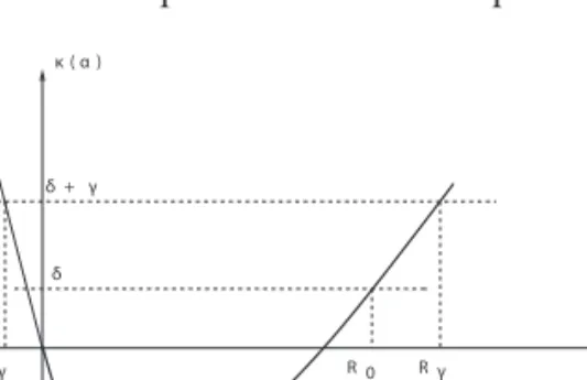
A crucial equation (in a) for this risk model turns out to be
a
( = +
k ) d g, (13)
where k(a) := l[ fY (– a) – 1] – ca. It has a unique negative solution – rg < 0. In addition, under a light-tailed assumption on the claim size distribution, it also has a positive solution Rg > 0 in the domain of convergence of fY(·) (cf. Figure 2). Note that for g = 0, (13) reduces to the well-known Lundberg
fun-damental equation of the compound Poisson risk process.
κ ( α )
δ δ + γ
The roots of the above equation are the negative of those of (13). Hence, the solution of (10) is of the form
(
L x + R
-; )b =C e1 rgx C2e gx, x#0
V (15)
for some constants C1, C2. Due to limx " – 3V (x; b) = 0, one immediately deduces C2 = 0.
For the middle layer 0 # x < b, one accordingly obtains the same homoge-neous differential equation for VM(x; b), but with g = 0. Hence
(x
M R
-; )b = A e1 r0x+A2e 0x, 0#x#b,
V (16)
where the constants A1, A2 are still to be determined.
For the upper layer x $ b, the same procedure results in a second-order differential equation in x for VU (x; b) with constant coeffi cients and character-istic equation (14), but with a non-homogeneous term that is linear in x. Hence
(x; )b D e D -Rg D x D x b U = 1 g + 2 + 3 + 4 $ rx x , e V (17)
for constants D1, …, D4. From the linear boundedness of V(x; b) it immedi-ately follows that D1 = 0.
For the determination of the remaining constants, the solutions (15), (16) and (17) are substituted into the IDE’s (10), (11) and (12). First, (10) does not yield any information. For (11), equating coeffi cients of e – nx leads to
R 0.
A1 1 A 1 C 1
0 2 0 1
+ + - + g =
n r n- n r (18)
As for (12), equating the coeffi cients of x yields
. D3 = g+d
g
(19)
With D3 determined, by equating the coeffi cients of e – nx along with the use of (18), we arrive at r R R R 2 g A1 b A b D R b D b 1 0 2 0 4 0 0 + + - - - - = + -r - -n n n n n n g d g n g , e e e a k (20)
while equating the constant term results in
g 2 D D c R b 4 - = + + -ge d g gd abd- lnk. (21)
In addition, the continuity of V(x; b) at x = 0 and x = b leads to the two further equations
0, A1+A2-C1 = (22) R -R + 4 . e A b D b D 1 0 + 2 2 - = -g d g g 0 -A r b e e b (23)
Therefore, we now have a system of the fi ve linear equations (18), (20), (21), (22) and (23) for the fi ve remaining constants A1, A2, C1, D2 and D4. This fi nally gives, after some elementary algebra and using equation (14),
r g g + g g g ( ; ) 1 / 1 / ( 0 x b e R R R e x L b R b x 0 0 0 0 0 0 0 0 0 0 # = - + + r r -r r r r R +r R -R ) , , e V (x r r g g R + g g g g ; ) / / ( ) ( ) , . b e R R e e x b 1 1 0 M b R b x R x 0 0 0 0 0 0 0 0 0 0 0 0 # # = - + + - -r r -r r r R +r R -R R R V e (24)
The result for VU(x; b) is also explicit:
( ( ( b; x b Rg b x g ; ) ( ) ; ) ), , b R dx d b V b x b 1 ( ) 1 U M b M $ = - + -+ - -= g d g g d g + + x x -e x V _ if V p
where VM(b; b) and dxd VM(x; )b x=b can be determined from (24).
Remark 2.1. The crucial result above is formula (24), which gives V(x; b) =
E[DM, d(x; b)] = E[Dd(x; b)], since for 0 # x # b there is no action at time 0 regardless of whether or not it is an observation time. However, even if one would eventually only be interested in this middle layer, the consideration of all three interacting layers was necessary to determine the involved coeffi cients in the present approach. Note that (24) is expressed solely through the roots of equation (14) for different values of g. Furthermore, it is ‘almost’ of the
form h(u) / h⬘(b) for some function h(·), which is the known form of V(x; b) for a general class of Markov processes that are skip-free upwards (see for instance Gerber et al. [8]). Formula (24) can hence also be seen as an adaptation of such a form for a model with certain types of upward jumps, in view of the random walk C(Zk) (k ! N) with state space R. See also Remark 4.4.
From Figure 2 it is easily seen that for g " 3 we have rg " + 3 and Rg " n so that (24) tends to (x R R r r R -V R 0 0 0 ; ) ( ) ( ) ( ) ( ) , 0 , b e R e x b b x 0 0 0 0 # # = + + -+ - - -n r n 0 0 0 n n b x r r e e
which is indeed the corresponding formula for the classical continuous-time risk model (see for instance Gerber & Shiu [9, Eqn. (7.8)]).
Remark 2.2. In principle, the method presented in this section extends to the
case of Erlang(n) observation intervals, to more general claim size distribu-tions as well as to the determination of higher moments Vm, d(x, b). However, this will typically lead to considerable computational effort, as one has to keep track of all three layers for each of the n exponential stages. In particular, 3n IDEs will have to be solved simultaneously and the complexity of these equations will further increase with the order m of the dividend moments as well as the claim size distribution. In Section 3 we will investigate an alterna-tive approach that allows to avoid these diffi culties.
3. METHOD 2: DISCOUNTEDDENSITYOFINCREMENT gd ( y)
We now follow another approach based on the increment of the uncontrolled process {C(t)}t $ 0 between successive observation intervals, exploiting the random walk structure of {C (Zk)}3k = 1. This will simplify the analysis to some extent. In this setting, time 0 is a fi rst observation point, so we can now directly work with defi nition (3).
Suppose we want to keep track of both the length of the interval Tk =
Zk – Zk – 1 and the change in the surplus between time Zk – 1 and Zk– (k = 1, 2, …). Due to the Markovian structure of {C(t)}t $ 0, this sequence of pairs is i.i.d. with generic distribution (T,
/
iN T=(1)Yi-cT) and joint Laplace transforms s T Y cT Y l ( ( d - i 1 - ) - i 1 Y E - T N T=( i E -d-cs T) E N T=( i| =E -[l+ -d cs- f ( )]s T . ) ) e = e e e 8 / B : 9 / CD 7 A (25)
On the other hand, one can also write
( s d 3 g Y cT ( d - i 1 - ) 3 E - T = -sy y dy) -( N T i =) e , e 8 / B
#
(26)where gd(y) (– 3 < y < 3) represents the discounted density of the increment
i i=1 Y cT ( N T -)
/
between successive observation times, discounted at rate d with respect to time T. This quantity will be particularly useful in the sequel.3.1. Exponential claim sizes and exponential observation times
Let us fi rst again return to the case that Y and T are both exponentially dis-tributed with mean 1/n and 1/g, respectively. Then (25) becomes
cT s - Yi ) T d - i =1 -E e , cs ( s = + + - - nn + g l d l g ( N T) 8 / B
which by the use of partial fractions can be written as cT R s R - Yi R ) T d - i =1 -E ( ) ( ) ( ) ( ) . e c s cR R s R ( = + + - + + -+ r g r r r g ( N T g g g g g g g g g g g g n ) n r c m r f p 8 / B (27)
Comparing (26) and (27), it is then clear that
R ( R R R R c d y) c ( ) { Rg I{ ( ) ( ) ( ) , g = + Iy<0} y y>0} 3<y<3 + + + - -g r g r r g g g g g g g g g g g ery n n e r r
-is a two-sided exponential density which -is defective when d > 0. We can now
condition on the pair (T1, i =11 Yi cT1) ( N T )
-/
to arrive at ( V ( R R y R R R R y ; x b ; ; c r r ( V y y R g g ( ( 3 x ; ) (( ) ) ) ( ) ( ) ( ) ( ) , 0 b c b x b c V b V b x b b x b x y 0 # # = + + - - + + + + + + + -- -r g r r r r g r r g g g g g g g g g g g g g g g g g ) ) ) . -n n n y dy x e x 0 e e dy dy r r 7 A#
#
#
(28)While the third integral term in (28) is a standard convolution, the fi rst two integrals resemble those arising in derivations for the dual risk model under a dividend barrier (see e.g. Avanzi et al. [6, Eqns. (2.3) and (3.1)]).
Applying the operator (d / dx – rg ) (d / dx + Rg ) on both sides, one can trans-form (28) into a second-order homogeneous differential equation in x for
V(x; b) with constant coeffi cients which has a solution of the form (x
V ; )b = A e1 a1x+A e2 a2x, 0#x#b. (29)
The constants A1, A2 and a1, a2 still have to be determined. Substituting (29) into (28) and matching the coeffi cients of the various exponential terms, one obtains the equations
R R 1, R R + a a ( ) ( ) ( ) ( ) 1 2 c c i 1 1 i i + - + + + = = g n r r g g g g g g g g g -, n , r r (30) a a a a A e A e 1 ab ab 1 1 1 2 2 2 1 2 - + - = rg rg rg, (31) R a R a 0 A1 1 A 1 1 2 2 + + + = g g . (32)
Equation (30) implies that a1, a2 are the roots (in z) of the quadratic equation R
R +( - ) - 2 = c c .
rg g rg g z z gn +g z (33)
Since rg and –Rg are roots to the quadratic equation (14), by Vieta’s rule they satisfy R c and c R ( - = rg g = +d n g g l+ +g d ) -g n. r
Applying these relationships to (33), one verifi es that indeed a1 = r0 and a2 = –R0. In particular, a1 and a2 are independent of g. The constants A1 and A2 now follow from the system of the two linear equations (31) and (32) and one fi nally again obtains (24).
The use of the discounted density gd(y) turned out to simplify the analysis as compared to the IDE approach of Section 2, as only the middle layer needs to be considered. In the next subsection we extend this method to higher dividend moments for Erlang(n) observation intervals and claim sizes with rational Laplace transform.
3.2. Higher moments of discounted dividends and Erlang observation times
When the observation interval T is Erlang(n) distributed and the claim size Y has an arbitrary distribution, the joint Laplace transform (25) has the representation
cT s - Yi (s ) T d - -cs Y 1 i = E f )] ( ) . e ( = + - + -g l g ( N T d ) [ n 1 c m 8 / B (34)
The zeros of the denominator inside the bracket on the right-hand side, namely the roots of the equation (in z)
l (Y
d z
( ) ) 0
c -z l+ +g + f = , (35)
are the negative of those of equation (13). In particular, there is a unique positive root rg > 0.
Recall (26) in connection with (34). Using the notation
( y -( ( ) { + y) d - + { , g y) = gd, Iy<0} gd, Iy>0} -3<y<3, (36)
along the same line of arguments as in Section 3.1, an integral equation for the m-th moment of discounted dividend payments can be obtained as
(37), , , m m m y ( k, ; ( ( ( ( x y; d d d b x k m m m - -3 x m ; ) ) ( ; ) ) ( ) ) ( ) ) , V b V b b g y dy V b g y dy V b g y dy x b k 0 , , , k m m b x 0 # # = -+ + + -d d d d = -- + y x b-x x 0 0 a k 7 A
/
#
#
#
for m = 1, 2, …. Here the quantities gmd, – (·) and gmd, + (·) refer to a discount rate
md instead of d.
Remark 3.1. Also in this approach one can obtain the moments of DM, d (x; b) (for which time 0 is not an observation time). The corresponding adaptations lead to , , , , m m m m y ( ( ; x x y ; ( ( ( ( ( ( ( x x y k k k -) ( ) ) b b b -+ -d d d d ) ) y b y , , , k m m k m k m m + + 3 3 m m m x m m ; ) [ ] ( ) ) ) , 0 ; ) [ ] ( ) ) [( ) ] ( ) ) ( ) , V b b b g y dy V g y dy x V b b b g y dy b b b g dy V g dy x b k k < > , , , , k m b x x b x k m x b x b 0 0 0 = -+ = -+ - -+ -d d d d d d d = -= -x ; , ; ; , d x 0 V V V x y y a a a k k
/
/
#
#
#
#
#
for m = 1,2, … . For 0 # x # b, the expression obviously coincides with the one where time 0 is an observation time. Hence the solution of (37) also leads to the formulas for x < 0 and x > b for the moments of DM, d (x; b).
The quantities gd, – (·) and gd, + (·) will not always have a tractable form, but if
fY(·) has a rational Laplace transform, i.e.
( ( ( , s f ) ) ) Q s Q, s Y r 1 2 1 = r - , (38)
where Q1, r (s) is a polynomial in s of degree exactly r with leading coeffi cient of 1 and Q2, r – 1(s) is a polynomial in s of degree at most r – 1 (and the two polynomials have distinct zeros), then it is shown in [1] that
( j +( B y r -, , d- y) ( ) ! and d y) ( 1) ! , g B y e g y 1 j n ij j n i r R 1 1 1 = = = = = g -j-1 j-1 * e g,i y - -j j
/
/
/
(39)where – Rg, 1, …, – Rg, r are the r roots of equation (35) with negative real parts (with fY(·) analytically extended beyond the abscissa of convergence), and the constants Bj* and Bij are given by
j n-j R n j ( ( l=1 ( 1) ( ) ! ) [ )] 1, 2, , B ds d Q s j n 1 , , j j r l r n 1 s c f = -- g = r = g ) s + -n n g , n n , a k
%
(40) andR n n ( j s , s , l=1 ( ) ! ( ) ) [ )] , , , , ; , , , . B d d Q i r n 1 1 2 1 2 , ij j j r l r n s R 1 , c f f = - - + g g g g ( n s i = = n j n n = -s -r l!i a k
%
(41)Since the above quantities depend on d, we write rg, m, Rg, i, m, B*j, m and Bij, m if
d is replaced by md.
If one now applies the operator (d /dx – rg, m )n
%
i =r 1(d/dx + Rg, i, m ) nto both sides of (37), it can be seen thatVm, d(x; b) satisfi es a homogeneous differential equation of order n(r + 1) in x with constant coeffi cients and has a solution of the form , i , md(x; ) A m , 0 , V b ea x b i n 1 , i # # = m = ( +1) x r
/
(42)for constants {Ai m, }i =n(r1+1) and i=1 ( ) n +1
a r
{ i m, } . We directly substitute (42) and the
densities (39) into the integral equation (37) and perform some straightforward but tedious calculations. Omitting the details, the fi rst integral on the right-hand side of (37) is evaluated as
l , g l ( i , , k k r, 1 + g m i -k j x m 1 m -d d 3 m-k m m b -[ ( )] ( ; ) ) ( ; ) ( ) ! ( ) ! ( ) ! ( ) ! ( ) . x V b b g y dy V b b B b b e k k 1 1 1 , , * k m b x k m j m j i n l i j l i n i i 0 0 1 , - -= -d r = -= = = = -- g rm- + - +k j l 1 - l e m b m i x -y j a a k k > H
/
/
/
/
/
#
(43)Similarly, the second integral in (37) is
, m , , j j m m ( y , , 1 g g r a ; i 1 , d g i -a ( x , , m m p m p l m a b -( ) ) ) ( ) ( ) ! ( ) ! ( ) . b g y dy A B e A B b e b e 1 1 1 1 a , , ( ) , ( ) b x i i n i m j j n m p n j i n m j l i j l i n i i 0 1 1 1 1 1 1 , , , i p m + = -- -d r -+ = = = = - + -- g V l m 1 m = + = b e r x m ) ) r x i x -r r f f p p
/
/
/
/
/
/
#
(44), m ( , p m y A A ; 1 d a a , m i j i R + -j ) y 1 x , , p m p m a ( ) ( ) ( ) ( ) ! ( ) . b g dy B e B x e 1 a , ( ) , , , , ( ) , , , , , m i n k m i m kj j n k r p n k m kj m j i n i n k r k m i 0 1 1 1 1 1 1 1 1 , , i -= + -+ + d g g g = = = = + = = = - - g V R R R r m r , m k + x m i x -x f f p p
/
/
/
/
/
/
/
#
(45)Incorporating (43), (44) and (45) into (37) and equating the coeffi cients of
1 er xi- g,mx yields l l , , j j m A , g l a , i i 1 , , p k m ! j m 1 - +1 + , g m , p m ( ) ( ) ! ( ; ) (( ) ( ) !) ! , , B b e V b b B k j b i k 1 1 1 1 2 a ( ) , m p n j i n j l l i j l k m j i n m k j l l i j l 1 1 0 1 1 , p - - -= - -- + -= g d = + = - + = = -= = - - + r r m l l m * * , r m f m b n r j . f a p k
/
/
/
/
/
/
(46) Note that we have separated the term Vm, d (b; b) and used (42) at x = b in obtaining the above equation. Similarly, by equating the coeffi cients of eai,mxwe arrive at , j m a , gm j a j ( ) ( ) , , . B R B 1 1 , , , , i j n i m kj j n k r 1 - 1 1 + = g = = = 1 , k * , , (n ) 2 m m f + m + i = r r
/
/
/
Due to the representation (26) and the form of the densities (39), the above equation implies that for each fi xed m = 1, 2, …, i =1
) ( nr+1
a
{ i m, } are roots of the
equation (in z) m Y - i 1 -E e dT-z( N T=( i cT) =1, ) 8 / B (47) which is the Lundberg fundamental equation of the present compound Poisson risk model under Erlang(n) observation intervals (this is natural in view of the embedded random walk structure of the uncontrolled process {C(t)}t $ 0 observed at discrete time points).
Finally, equating the coeffi cients of xi -1e-Rg, ,k mx gives
a Ap, , ,k m p m, g ( ) 0, 1, 2, , 1, 2, , B r n ) , m p n j kj j i n 1 f f + = = = . ( m 1 + ; R r = = k i
/
/
(48)Hence, for each fi xed m ! N, a i =n(1 1) +
{ i,m} r are obtained as the roots of (47), and
1 i =n( 1)
+
and (48). Then a complete characterization of Vm, d (x; b) is given by (42). In view of (46) this procedure is recursive in m.
Remark 3.2. From the Lundberg equation (47) along with the representation
(34), one observes that the roots i =1 n( 1)
a +
{ i, } r
m are independent of g when claims
have rational Laplace transform, as long as the observation intervals remain exponential (i.e. n = 1). Indeed, they are the roots of (35) with g = 0 (and md
instead of d) and are hence the negative of the roots of (13) with g = 0 (also
with md in place of d). However, for arbitrary Erlang(n) observation intervals, 1 i = n( 1) a + { i, } r
m will in general not be independent of the value of g.
4. METHOD 3: DISCOUNTEDDENSITYOFOVERSHOOT hd( y | x; b)
We now present yet another, although related approach to analyze this model. This method is based on the fact that, from any present surplus level, further dividends can only be collected if the uncontrolled process overshoots level b before it becomes negative at an observation time. As we shall see towards the end of the section, this method leads to expressions from which certain classical results can be retrieved as special cases. These include the Laplace trans-form of a two-sided upper exit time and the expected discounted dividends paid until ruin.
Assume that time 0 is the fi rst observation time and let kb* = min{k $ 1 : Ub(k) > b} be the number of observation intervals before the fi rst overshoot of the process {Ub(k)}3k = 1 over level b. Clearly tb* = Zk*b is the fi rst time a dividend
payment is made as long as tb* < tb (i.e. ruin has not occurred yet). In the spirit of Gerber & Shiu [9], suppose a ‘penalty function’ w*(·) is applied to the fi rst overshoot of {Ub(k)}3k = 1 over level b avoiding ruin until then and defi ne the quantity b ( (0) b d E b ( ; )x b e w U k( b b I) {b< b} W x, 0#x#b.
x
= t - t t = - ) ) ) d ) ) : D (49)Recall the discounted density gd (y) from (26) in its decomposed form (36). Akin to the derivation of (28), we have by conditioning
( ( ( ( ( x y y ; ; x ( - -x * 3 x ; ) )) ) ( ) ) ( ) ) , 0 . b y y dy b y dy b y dy x b w b b x 0 0 # # = - + + + -d d d -+ x x x g g g , , , d d d - b x x
#
#
#
(50)In Section 4.1 we will solve this integral equation for claim sizes with rational Laplace transform along the same lines as the one for Vm, d (x; b) in Section 3.2 was dealt with. We shall now fi rst show how the quantity xd(x; b) can be used to study the dividend moment function Vm, d (x; b).
Suppose in general that xd(x; b) can be expressed in the form ( x; (x; )b = 3w y)h ( | b dy) , 0 #x#b, d d x * y 0
#
(51)where hd (y |x; b) is the discounted density of the overshoot over level b avoiding ruin. Then by conditioning on such a fi rst overshoot, one arrives at
, md(x k, ( k x;b -3 m ; ) ( | ) , 0 . V b k y h dy x b k m m m 0 0 # # = d = ; V b b) d y a k
/
#
(52)Moreover, for m = 1 this simplifi es to
( ; V b (x ) x; V ; )b = 3 y+ b hd( |y b dy) , 0 #x#b. 0 7 A
#
(53)Putting x = b in (52) and solving for Vm, d (b; b) yields
, md( , m k h h 3 3 m ; ) ( | ; ) ( ( | ; ) . V b b b b dy k V y b b dy 1 1 k m m k m 0 0 1 0 = - d d d = -; b )b y y a k
/
#
#
(54)Thus, (54) is a recursive formula to evaluate Vm, d (b; b) for all m, and then
Vm, d (x; b) for 0 # x < b can be obtained via (52).
Remark 4.1. The representations (52) and (54) are valid for arbitrary
distribu-tions for the claim size and the observation intervals.
Remark 4.2. Assume again that both the claim sizes and the observation
inter-vals are exponentially distributed with mean 1/n and 1/g, respectively. Then,
skipping the details, the solution of (50) leads to
R x r R R -r r ( -r (x R R R -0 0 0 0 R R y r 3 ( ) ( ) ( ) ( ) ( ) ( ) [( ) ( ) ] , e dy e e e R e x b 0 b R b x 0 0 0 0 0 0 0 0 0 # # = + + - -- + + -d r r -g x g g g g g g g g y ; )b w ) r , r r r * a
#
k and therefore x R x ; r R R -r r -r b R R R -0 0 0 0 R R y r ( | ) ( ) ( ) ( ) ( ) ( ) ( ) [( ) ( ) ] ; . h e e e e R e y>0 0 x b b R b x 0 0 0 0 0 0 0 0 # # = + + - -- + + -d r r -g g g g g g rg g g , y r r rThis factorization form makes it particularly easy to compute the integral terms in (52) and (54).
4.1. Solution of xd(x; b) for claims with rational Laplace transform
If (as in Section 3.2) the claim sizes have rational Laplace transform and the observation intervals are Erlang(n) distributed, then (50) can be solved to give
j (x 1 , 0 ea x b ( ) i i n 1 i # # = d = + x ; )b x , r
/
(55) where i=1 i=1 ( ) ( 1) nr+1 nr+ a a { i} /{ i 1, } , and i=1 ( ) nr+1{j }i are the solution of the system of n (r + 1) linear equations consisting of
l j j i j- +l 1 a i p l r y y b p) 3 ( ( ) ! ( ) ! ( ) ! ( ) , , , B b e B b e w y dy i n 1 1 1 2 a ( ) p n j i n l i j l j i n l l i j j 1 1 0 p f - -= - - = g = + = = = = - -j g , l * * * l r , r j a k
/
/
/
/
/
#
(56) p ap ( ) 0, 1, 2, , ; 1, 2, , B r n ( ) , p n j k j i n 1 1 f f + = g = + = k j . R r j k = i =/
/
(57)For exponential observation times (i.e. n = 1) one can get more explicit results and we shall restrict ourselves to this case for the rest of this subsection. Equa-tions (56) and (57) then reduce to the set of linear equaEqua-tions
( )b ( p y y r ) w p b 3 * a e e dy, 1 a p r 1 1 p j - = = + - g rg 0
/
#
(58) ( )b p 1 ap 0, 1, 2, , , R r 1 , p r k 1 f j + = g = + = k/
(59)where we emphasized the dependence of {j }i ir=+11 on the barrier b. For i =
1, 2, …, r + 1, we defi ne hi to be the cofactor of the (1, i)-th element of the coeffi cient matrix of the above linear system (with (58) listed in the fi rst row). It is instructive to note that {h }i ir=+11 do not depend on b, since b only appears
in the fi rst row of the above-mentioned coeffi cient matrix. Moreover, each hi can be computed via the determinant of a Cauchy matrix with the appropriate sign (see the Appendix of Gerber & Shiu [10]). Then, solving the system by Cramer’s rule followed by cofactor expansion (along the i-th column for the numerator and along the fi rst row for the denominator) in the evaluation of determinants, we arrive at ( r ( , p y p=1 p a ) ) , . b e w dy e 1 a 1 2 1 i y p r b i 0 1 j = -3 -+ g h r h g * , i = f r +, a k
/
#
(60)Incorporating (60) into (55) (for n = 1) gives ( r (x 1 1 y y -) w i i 3 i i 1 1 = = a ; )b e dy 0 . e x b 1 a r i b r 0 i i # # h h = -d + + g x r * g ea , x a k
/
/
#
Due to relationship (51), one concludes that hd (y|x; b) admits the factorization as a product of a function of y, a function of x and a function of b as
; x r ( ( b s | ) ) ) , 0; 0 , h e b x y> x b y 2 1 # # = d rg - g s (y (61) where ( h ( h s x) iea and s b) a ea . i r i i r i 1 1 1 2 1 1 i i = = -= + = + r r g g x b
/
/
Remark 4.3. The defi nition (49) together with the representation (51) with
w*(·) / 1 means that x ( ( h 3 i i 1 1 = = s s a ( | ; )b dy )) 0 b x e e x b a a i r i i r 0 2 1 1 1 i i # # h h = = -d + + r r g g b x , y
/
/
#
is the Laplace transform of the time of the fi rst overshoot above level b avoid-ing ruin, when the initial capital is Wb(0) = x. If, for example, the claim size follows a mixture of exponentials with distinct means 1/n1, 1/n2, …, 1/nr , then a simple graphical plot reveals that, as g → 3, one can write rg → 3 and Rg, k → nk for k = 1, 2, …, r, so that
; x i i 3 i i 1 1 = = ( | ) , 0 , lim h b dy e e x b a a r r 0 1 1 i i # # h h = "3 g d + + b x y
/
/
#
(62) where i=11 + r{h }i are now calculated from the coeffi cients of the system (59) with Rg, k replaced by nk. Note that with g → 3, the time of fi rst overshoot over level b
avoiding ruin in the present model is essentially the time of fi rst upcrossing level b avoiding ruin in the classical continuous-time barrier model. Indeed, (62) coincides with Gerber & Shiu [11, Eqn. (A.9)].
Remark 4.4. It is also worthwhile to note that (61) implies the normalized
dis-counted density of the amount of overshoot to be exponential with mean 1/rg, regardless of the initial capital x and the barrier level b.
Finally, substitution of the factorization (61) into (53) leads to ( ( x ) b ( ( V ; ) [ ) ] ) , 0 . b b x x b 2 1 1 # # = -rg s s s
As expected, the optimal barrier level b = b* which maximizes V(x; b) with respect to b is independent of the initial surplus 0 # x # b*. Note also that in the limit g " 3, (due to rg " 3) the denominator in the above expression is
⬘( s ( )]b = i = i b) s aa a [ ( ) , lim b lim ea a i r i i b i r i b 2 1 1 1 1 1 1 i i h h - -"3 "3 g g = + = + rg r g g r e = s
/
/
with the understanding that {h }i ir=+11 are calculated at the limit as g " 3 (see
Remark 4.3). Hence, in the limit one obtains the well-known form V(x; b) = s1(x) / s1⬘(b) of the continuous-time model.
5. ONTHEOPTIMAL BARRIERCHOICEFOREXPONENTIAL
INTER-OBSERVATIONTIMES
In this section we will discuss the issue of the optimal dividend barrier further according to the defi nition (2), i.e. time 0 is not an intervention time. For the entire section we assume that the inter-observation time T is exponentially distributed with mean 1/g. Let us start with the case of exponential claims. Example 5.1. Assume the claim size Y is exponentially distributed with mean 1/n.
Since in equation (24) only the denominator depends on the barrier level b, one can identify the optimal barrier b* which maximizes V(x; b) for a given initial capital x by minimizing the denominator with respect to b. This imme-diately leads to R = 0
r
r
R R , ( ) ( ) ( ) ( ) max ln b 0 1R R R 0 0 0 0 0 0 02 + + + - -r r2 ) g g g rg , r * 4 (63)which generalizes Gerber & Shiu [9, Eqn. (7.10)]. Also, one readily checks that
) = ) ( ) . dx d V x 1 x=b ; b (64)
At the same time, b* is the only value b for which (64) holds. ¡ Recall that in the classical continuous-time model dxd V x b( ; )e 1
x=b= for all b,
whereas in the above example with exponential observation times and exponen-tial claims, this derivative was equal to 1 at the barrier only if the barrier is optimal. In the sequel we will show that this property holds more generally.
With a general claim size density fY(·), differentiating (11) and (12) and evalu-ating in x = b, together with the continuity conditions VL(0; b) = VM(0; b) and
VM(b; b) = VU(b; b) that were established in Section 2 we obtain
( ( ( ( x x x x U U y y ; ) ; ) ; ) ; ) b b y b b y ; ; ; ; d d b b b b b b b b 3 3 ( ) ( ) ( ) ( ) ( ) ( ) c dx d V dx d V dx d V b dx d V b c dx d V dx d V dx d V b dx d V b 0 0 M M M b Y L Y M b Y L Y 0 0 = - + + - + -= - + + + + - + -= = = = = = = = l l g g l l ( ( ( ( 2 2 b b l l 2 2 , x x x x y y y y x x x x x x x x ) ) ) ) . dy dy dy dy f f f f c c c c m m m m
#
#
#
#
Since we know from (8) that the derivative of V(x, b) in x = b exists, from the above expressions it is clear that the second-order derivatives of VM(x, b) and
VU(x, b) in x = b match (i.e. the second derivative of V(x, b) in x = b exists) if and only if dxd VM(x; )b x=b= dxd VU(x; )b x=b=1.
If V(x, b) is differentiable in its second component b, then an obvious neces-sary condition for optimality is 22bV(x; )b =0 at b = b* for x ! R. But we will now show that this implies (64). For fi xed b, Dynkin’s formula (see e.g. Rolski et al. [14]) can be applied for V(x; b) and states that
( - l+d ( (s y; ( ); ( ) ) ); t 0 ; ( (C C C C ( t d y 3 t ( ( ( ( ) ) ) e V b V b c x V b V s b ds ) s C s Y 0 2 0 2 - d + -l x ) ) ) f dy V -; ) e b = x c m
#
#
defi nes a zero- mean martingale (note that the generator of the uncontrolled surplus {C(t)}t $ 0 applied to e – dtV(x; b), namely
y; (x (x ( - b) ( V ; ) ( d)V ; ) 3V c x b b Y 2 2 - l+ +l x f y dy) , 0
#
(65)is part of the IDEs (5), (6) and (7) for V(x; b) in Section 2).
Let us condition on the observation time T = t and replace (65) by the specifi c inhomogeneities, then for 0 < b < b⬘ we obtain
t = ( ( ⬘) x x d ( ); ( ); ( ( ); ( ; ( ); ( t d C C t -V V ( ( ( b C E E ⬘ ⬘ ⬘ ⬘ ⬘ ; ) ; ) ( ) ( ( ); ) ( ) ( ); ) { ( ) ( ) ) [ ( ) ( ]} { ( ) [ ) ( )]} . b V C b V C t V C s b V C s I V C s b V C s b V b V I V C s b C s b V b I T ⬘ ⬘ { ) } { ) } { ) } s t s s b b s b 0 <0 > < - = -- -+ - + - - -+ - - + # - g g g [ [ ; ; ; b b ] ] b e b b b b ⬘ ds e b ` j 8 9 CC
#
(66)Before dividing by b – b⬘ we look at g{V C s);( ( b)-[C s( )- +b V b( ;b)]}I{b<C(s)#b⬘}
and notice that for | b⬘ – b| small we can apply a second-order Taylor expansion around b, for a fi xed surplus path,
( b [ s -) ] (x + -b (x (s C V (s V ( ); ) ( ; ) ; ) [ ) ] ; ) V C b V b b x b C x b 2 b 2 2 2 2 2 2 2 = + z = = x x
for some z ! (b, b⬘) such that the second derivative exists and is fi nite. Now let
us divide equation (66) by b – b⬘, (67) -b b t -= ( ( ( ( ⬘) x x x x -+ z d ( ); ( ); ( ( ); ( ; ( ) ( ) t b d g C C t -V V V V ( ( [ ( { C s b - - 2 b (s 2 E E ⬘ ⬘ ⬘ ⬘ ⬘ ⬘ ⬘ ⬘ ⬘ ⬘ ; ) ; ) ( ) ( ( ); ) ( ) ( ); ) ( ) ( ) ) ( ) ( [ ] ; ) ; ) [ ] . b b b V C b V C t b V C s b V C s I b V C s b V C s b V b V I b C s b b s I T 1 ⬘ ⬘ { ) } { ) } ) ] ) } s t s s b x x b C b 0 0 2 < > < 2 -= -+ -+ -2 2 2 2 # -= = g g ; b; C b b e b b b b b b b b ⬘ ds x + e x b d n < = V X W W WW V X W W W W (
4
#
Note that b ( ( -b x + x -z ( ) V b [ ( V ( ) { C s b - - 2 (s 2 ⬘ [ ] ; ) ; ) [ ] b C s b b s I ⬘ ) ] ) } x x b C b 2 < 2 -2 2 2 2 # = = C b x xtends to zero if b " b⬘ exactly if limb"b⬘ 22xV(x; )b x=b=1, or equivalently
(x b⬘ V ; )b = 1. x = 2 2 x When writing ⬘ ⬘ ⬘ ⬘ ⬘ ⬘ ⬘ ⬘ ⬘ ( ; ) ( ; ) ( ; ) ( ; ) ( ; ) ( ; ) b b V b b V b b b b V b b V b b b b V b b V b b = +
-in (67) we get that 22bV(x; )b =0 for some b = b* and arbitrary x ! R can only
hold if (64) holds.
Because V(x; b) is linearly bounded and monotone we are allowed to inter-change expectations and the limit b " b⬘ and can conclude that a positive maximizing barrier height b* implies (64), which itself implies that V(x; b*) is twice differentiable in x at x = b*. These arguments are also valid for b > b⬘ and b " b⬘, therefore the fact that V(x; b*) is twice differentiable in x at the barrier turns out to be a necessary criterion for the optimality of the barrier in this model.
6. NUMERICALILLUSTRATIONS
Let us now look at some numerical illustrations. Consider fi rst the case of exponential claims with mean 1/n and exponential inter- observation times
FIGURE 3: Optimal barrier b* as a function of g for exponential claims and exponential inter- observation times with c = 6, n = 3, l = 15, d = 0.05.
FIGURE 4: V(x; b) for three barrier levels b = 5 (dotted line), b = b* = 7.379 (solid line) and b = 10 (dashed line) and parameters c = 6, n = 3, l = 15, d = 0.05, g = 10.
with mean 1/g. In this situation, the optimal barrier level b* can be calculated via formula (63). Figure 3 depicts b* as a function of g for a particular set of parameters. As can be expected, b* increases with g, as a larger value of g leads to more frequent observations of the process, which implies a higher chance of observing early ruin, and as a result a higher b* is required for safety (other-wise ruin may occur before dividends are paid). Let us now fi x the value of
g = 10, for which the optimal barrier level is b* = 7.379. Figures 4 and 5 give V(x; b) for three different barrier levels b and illustrate the smooth-fi t property
FIGURE 5: First and second derivative in x of V(x; b) for three barrier levels b = 5 (dotted line), b = b* = 7.379 (solid line) and b = 10 (dashed line) and parameters c = 6, n = 3, l = 15, d = 0.05, g = 10.
of the maximizing barrier b*. We see that the fi rst order derivatives with respect to x fi t together in x = b for each of the three barrier levels. However, only for the barrier level b* we have that V(x; b) is twice differentiable in x and the necessary criterion (64) for the optimal barrier level b* holds.
Next, we compare the values of the expected values V(x; b) and standard deviations SD(x; b) of the total discounted dividend payments until ruin for our model with random observation times to the ones of the classical con-tinuous observation model for three different parameter sets. At the same time, we investigate how much the values of V(x; b) and SD(x; b) are affected by the ‘randomness’ of the observation times. This is done by using observation intervals with Erlang(n) distribution, for which we fi x the expected time between observations (E[T ] = 2.5), but increase the value of n. Note again that for large n we approach the case of deterministic periodic observation intervals (i.e. the discrete-time risk model), yet utilizing the computational advantages of the random approach. We shall consider three different claim size distributions, each of which leads to an expected value of 1. Concretely, we consider a sum of two exponentials with mean 1/3 and 2/3 (Table 1), an exponential claim size distribution with mean 1 (Table 2) and a mixture of two exponentials (one exponential with mean 2 (mixing probability 1/3) and one exponential with mean 1/2 (mixing probability 2/3)) (Table 3). The variances of these claim distributions are 0.56, 1 and 2, respectively.
Note that all the above claim distributions have rational Laplace trans-forms fY(s) in the form of (38). Therefore, in producing the following tables, the algorithm in Section 3.2 for Erlang(n) observation intervals can be used. Our procedure is summarized below.
1. For various positive integers m (up to the order of dividend moments of interest), solve (35) with d replaced by md, which has a unique positive root rg, m and r roots with negative real parts, namely –Rg, 1, m, …, –Rg, r, m. 2. One may use (40) and (41) (with rg and Rg, i replaced by rg, m and Rg, i, m
respectively) to determine B*j, m and Bij, m. However, they also may be deter-mined as the coeffi cients in the partial fractions expansion