Constrained control using convex optimization

Constrained Control using Convex Optimization

by

John Marc Shewchun

B.A.Sc. Aerospace Engineering University of Toronto, 1995

Submitted to the Department of Aeronautics and Astronautics

in partial fulfillment of the requirements for the degree of

Master of Science in Aeronautics and Astronautics

at the

MASSACHUSETTS INSTITUTE OF TECHNOLOGY

@ Massachusetts

August 1997

Institute of Technology 1997. All rights reserved.

Author.

Department of Aeronautics and Astronautics

Q-

August 8, 1997

Certified by...

Eric Feron

Assistant Professor

Thesis Supervisor

Accepted by

Jaime Peraire

Associate Professor

Chairman, Department Graduate Committee

, .'NOLOGY

OCT

15 1W97

Constrained Control using Convex Optimization

by

John Marc Shewchun

B.A.Sc. Aerospace Engineering University of Toronto, 1995

Submitted to the Department of Aeronautics and Astronautics on August 8, 1997, in partial fulfillment of the

requirements for the degree of

Master of Science in Aeronautics and Astronautics

Abstract

Constrained control problems are ubiquitous. Since we cannot escape them, the only alternative is to develop "sound" methodologies for dealing with them. That is, we must provide methods that have specific guarantees as dictated by the problem, otherwise we cannot say with certainty that our control decision will result in a stable or safe system. In particular, two different, but related, constrained control areas are investigated. The first is the problem of Linear Time Invariant systems subject to nonlinear actuators. That is, actuators that have symmetric or asymmetric position constraints and possibly rate constraints. The second problem is the detection and resolution of aircraft conflicts. Both problems are very pressing in their own distinct ways. For the first problem a nonlinear state feedback methodology is developed that has guaranteed constraint satisfaction and global asymptotic stability. This is brought about by scheduling the gain to avoid saturation at all times, and is accomplished through a set of nested invariant ellipsoids that for each gain approximate the maximal invariant set. A comparison to sub-controllable sets and an application to the F/A-18 are given. The second problem is approached through a two phase method. Firstly, aircraft conflicts are detected by performing a worst case analysis of the situation through Linear Matrix Inequality feasibility problems. Once this is completed the resolution problem is approached by formulation as a convex optimization problem. The resulting strategy is highly combinatorial in its complexity. A possible solution to this problem is attempted by formulation of a lower bound obtained by convex optimization techniques.

Thesis Supervisor: Eric Feron Title: Assistant Professor

Acknowledgments

First and foremost I would like to thank Eric Feron for the opportunity to come to MIT and work on a very challenging research topic. Without his guidance this thesis would not have been possible.

Thank you to all of the members of the Instrumentation, Control, and Estimation group, both past and present. Your helpful discussions and most importantly your friendship made my stay an enjoyable one.

Contents

1 Introduction 15

1.1 Background and Previous Results . . . . . 18

1.1.1 Linear Systems with Pointwise-in-Time Constraints . . . . 19

1.1.2 Conflict Detection and Resolution . . . . .. 21

1.2 O utline ... . . . .. . .. . . . ... . . . .. 21

2 Preliminaries and Problem Statement 23 2.1 Convex Optimization and LMIs .... . . . . . . . . . 23

2.1.1 Schur Complements ... . . . . . . . . . . . . 25

2.1.2 Duality and the Quadratically Constrained Quadratic Program 25 2.2 Lyapunov Stability Theory and Invariant Sets . . . . 28

2.3 Constrained Control Problems ... . . . . . . . . . . 31

2.3.1 Asymptotic null controllability with bounded controls . . . . . 33

3 Nonlinear State Feedback for Constrained Control 35 3.1 Position Constraints ... ... ... ... 38

3.1.1 An Academic Example . . . . . 44

3.1.2 Limit Properties of Invariant Ellipsoids . . . . 46

3.2 Asymmetric Controls ... ... 49

3.2.1 Example of Asymmetric Control ... . . . . . . . . .... 54

3.3 Position and Rate Constraints ... . . . . . . . . . . . .. . 57

3.3.1 LQR Based Solution ... . ... 57

3.4 Comparison with Reachable Sets . .

3.4.1 Sub-Reachable Sets . . . .

3.4.2 Extension to Controllable Sets

3.5 Application to the F/A-18 HARV . .

3.5.1 Controller Design ...

with State Constraints .

. . . . 70

. . . . 70

. . . . 74

. . . . 77

4 Conflict Detection and Resolution

4.1 Conflict Detection ... ...

4.2 3-Dimensional Case ... . . . . . . . . . .....

4.3 Conflict Resolution ... . . . . . . . . .....

4.4 Computation of the Lower Bound .... . . . . . . . .....

5 Conclusions and Recommendations

5.1 Nonlinear Control for Nonlinear Actuators . . . ..

5.2 Convex Optimization for Aircraft Conflict Detection and Resolution . 83 84 93 97 102 109 109 111

List of Figures

1-1 Nonlinear Actuator Model ... . . . . . . . . . . . . 16

3-1 The Sets ,A4, and A ... . . ... ... . 36

3-2 Nested Ellipsoids ... ... ... 42

3-3 Nested Ellipsoids for Double Integrator . . . . . 45

3-4 States and Control for Double Integrator . . . . 45

3-5 Open Loop Unstable System ... 47

3-6 Asymmetric Ellipsoids for Spring Mass System . . . . 54

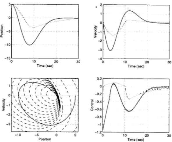
3-7 States and Control for Spring Mass System: Example 1 . . . . 56

3-8 States and Control for Spring Mass System: Example 2 . . . . 56

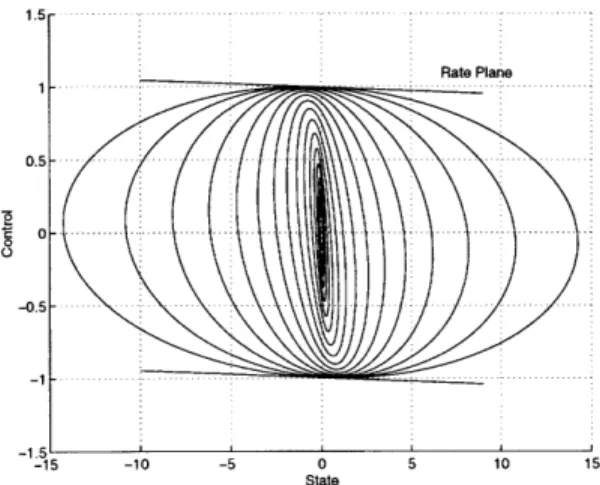
3-9 Invariant Ellipsoid Set for Single Integrator . . . . . 65

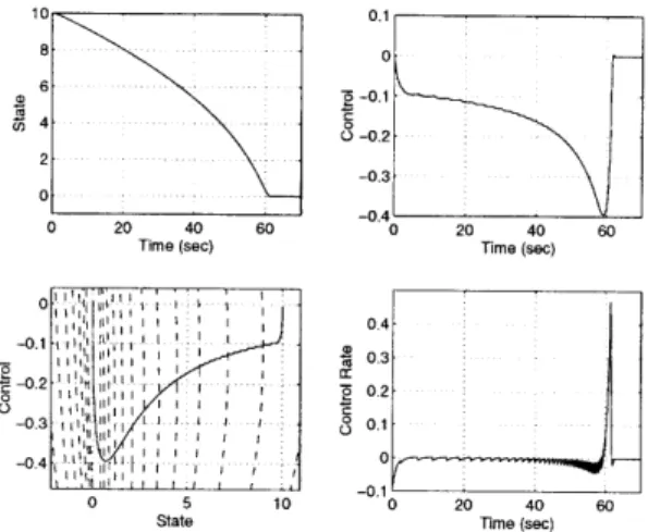
3-10 Performance of Single State System . . . . 66

3-11 LMI Invariant Ellipsoid Set for Single Integrator . . . . 70

3-12 Performance of Single State system with LMI Enhancements . . . . . 71

3-13 Sub-Controllable Set for Double Integrator . . . . 74

3-14 Performance for Sub-Controllable Set Controller . . . . 75

3-15 Sub-Controllable Set for State Constrained System . . . . 77

3-16 Performance for Sub-Controllable State Constrained Controller. . . . 78

3-17 F/A-18 HARV Nonlinear Model ... 78

3-18 Single Side Turn Response ... . . . . . . . . . 82

3-19 Control Surface Positions and Rates . . . . 82

4-1 Uncertainties in the Velocities ... . . . . . . . . . . . 85

4-3 Uncertain Acceleration . ... 91

4-4 3-Dimensional Case .. ... . 93

4-5 Relative Motion and Admissible Regions ... . . . . . . . . . . 99

4-6 Constraints on Aircraft Velocities ... . . . . . . . . . . 101

4-7 Frequency of Null Eigenvector ... . . . . . . . . . . . . . . 106

4-8 Example of a 4 Aircraft Conflict ... . . . . . . . . . . 107

List of Tables

3.1 3% Settling Times for Asymmetric Control Examples . . . . 55

3.2 Performance for F/A-18 HARV Example . . . . 81

Notation

Ik

The real numbers, real k-vectors, real m x n matrices. The nonnegative real numbers.

The positive real numbers. The nonnegative integers. The k x k identity matrix.

Transpose of a matrix M: (MT) j Mi.

Trace of M E Rnn, i.e., ZEn 1 Mii.

M is symmetric and positive semidefinite, i.e., M = MT and

zTMz > 0 for all z C Rn_.

M is symmetric and positive definite, i.e., M = MT

and zTMz > 0 for all nonzero z E Rn . M and N are symmetric and M - N > 0.

For M > 0, M 1/2 is the unique Z = ZT such that Z > 0, Z2 = M.

The maximum element of the matrix M.

Square matrix formed from the diagonal elements of M,

i.e., diag(M)ii = Mi., and diag(M)j = 0 for j # i. Block-diagonal matrix formed from the arguments.

The submatrix formed by the elements of the rows indexed by a and the elements of the columns indexed by 3. For example,

123

4 5 6 ({1,3},{1,2,3}) = 1 2 3

7

89

ellipsoidal set defined as E(M, ac) x E R " XTMX < oK .

ellipsoidal set defined as S(M, a, a) {x E Rn(x - a)TM(x- a) < a}.

ellipsoidal set defined as E-'(M, a) {x E Rn(x - a)TM-(x - a) < 1}.

hyperslab defined as 7-W(c) x

E

hyperplanes defined as P(c) = {x

E

standard n-dimensional Euclidean norm, i.e. x_I = XTX.

S(M, a) S (M, oa, a) 8-1(M, a) P1(c) P(C)| The The The The The The

Chapter 1

Introduction

Constrained control problems are ubiquitous. Whether it is the mechanical limitations of an actuator, or the amount of cash that a company has available for investment in a new venture, the control of any dynamic system will always involve real physical constraints on the states and inputs that must be considered. Sometimes, these constraints may be weak, in that, for all intensive purposes they can be ignored. However, in many cases they are severe and disregarding them in a control decision or design could easily lead to disaster. The point is that since they cannot be avoided, sound methodologies must be developed to deal with them. The point of departure for this thesis will be the constrained control of Linear Time Invariant (LTI) systems. In particular, systems that have nonlinear actuators or systems that have more general state and control constraints.

One of the most typical input constraints for LTI systems results from nonlinear actuators. Indeed, all actuators are nonlinear since they are unable to respond to an input above a certain level. These are hard constraints because the actuator simply does not respond if the constraint is violated. Fig. 1-1 shows a typical model of an actuator that has linear dynamics, position saturation, and rate limiting; which could be used to represent the servo that drives an aircraft control surface. The actual control input u will be a linear function of the commanded input u, only when

uc is within the saturation and rate limit bounds. However, when the actuator is

uc LINEAR u

ACTUATOR

----DYNAMICS

SATURATION RATE LIMITER

Figure 1-1: Nonlinear Actuator Model

be radically reduced, and the system could possibly be driven unstable. One such problem, that applies to pure saturation only, is know as integrator windup, where an integrator in the control loop builds up to a value greater than the saturation limit of the actuator. When the integrator finally begins to unwind the resulting control signal can become badly out of phase and result in severe oscillations, see pg. 79 in [76] for a brief discussion. It has also been observed that multiple saturations change the direction of the controls resulting in improper plant inversion [35]. Even more recently is the identification that actuator rate saturation poses a severe problem to modern combat aircraft. High performance aircraft are constantly pushing the limits of available performance. The phase lag induced by rate limiting has been shown to produce a significant tendency for Pilot Induced Oscillations (PIOs) [36, 29]. Yet another nonlinear actuator problem occurs when the position saturation limits are non-symmetric. This problem is present in a large number of actuation problems, yet few techniques have been developed that directly take asymmetric constraints into account. In response to these problems a wealth of techniques and methodologies have been put forward, and recently much renewed interest has taken place, see for example the recent journal [4].

Another important problem that can be cast in the constrained control of LTI sys-tems category is aircraft conflict detection and resolution. The definition of an aircraft conflict is quite simple. Given a portion of airspace, a conflict between two aircraft is declared when their predicted positions are such that both a specified horizontal and vertical separation parameter are infringed [30]. The separation parameters

rep-resent a desired safety margin which cannot be violated. Even before the conflict can be resolved it must be detected by analyzing the situation. Once the analysis technique has declared a conflict the resolution problem is to determine trajectories, for all aircraft involved, that will eliminate the threat of a collision. Thus we have a combined detection and resolution problem and the two are inseparable. Although the detection/resolution problem is quite simple in formulation, its solution is ex-tremely difficult due to the combinatorial nature of the problem. For two aircraft the situation is well understood, and analytical detection and resolution methods

exist [56, 42]. However, the worst case number of computations needed in the

con-flict detection problem grows with the square of the number of aircraft [69]. Even

more significant, the worst case number of computations in the resolution problem can grow as two to the square of the number of aircraft [18]. Motivation to provide new methodologies for dealing with this situation has been increasing. Most recently, under the concept of Free Flight, rigid airway structures and other constraints on

aircraft trajectories will be greatly reduced [3]. Aircraft will be allowed to plan their

own trajectories in order to optimize a range of flight variables. The resulting flex-ibility will require more sophisticated automated conflict detection and resolution. In particular both pilots and ground controllers, with the aid of automated systems, will be responsible for predicting and avoiding collisions. It is easy to see why such a problem is really a constrained control problem. In resolving a conflict there are really only two possibilities. Conflicts can be solved horizontally by issuing each aircraft a turn maneuver, or vertically by specifying climb and descent rates. It must therefore be taken into account that the aircraft have limits on rates of turn and climb [41]. Indeed, this is similar to the nonlinear actuator in that there are hard constraints on aircraft maneuverability. Furthermore, it follows that the condition that any two aircraft not violate a given separation parameter is a state constraint. Underlying this is the absolute necessity for safety. Human lives are at risk, and thus resolution methods must provide guarantees of safety. All of this poses a challenging constrained control problem.

inputs that satisfy the problem statement. Thus the problem of constrained control can be succinctly defined as selecting the best (in some pre-defined sense) possible admissible control such that the state constraints are never violated (i.e. the state is always admissible). Clearly, both of the problems described above fall into this description. Furthermore, we are really implicitly describing an optimization prob-lem. The term best implies that we will choose some performance index that is to be maximized. As we will see, one of the difficulties that follows from this is the repre-sentation of the admissible sets. Our approach will be one of convex approximation, that is defining all admissible sets in terms of convex ones.

In this thesis we will bring to light two methodologies for solving the constrained control problems described above. The first is a closed loop feedback control for deal-ing with nonlinear actuators. The second is a more general method for control that is motivated by and presented through the aircraft conflict detection and resolution problem. Underlying the two methods are two crucial goals. First, we desire numeri-cally efficient methods. By numerinumeri-cally efficient we mean that the methods must have guaranteed solution times and are possibly implementable in real time. Secondly, is the desire to provide as many guarantees on the solution in terms of stability and performance (i.e. optimality). As stated, one of the tools we will make large use of to

aid in this pursuit will be convex optimization. In short, convex optimization is any optimization problem for which the objective and constraints are convex functions. There are many benefits that arise from using convex optimization. An important one is the fact that any locally optimal solution is guaranteed to be globally optimal. Also, convex optimization problems have guaranteed computational solution times

[54].

1.1

Background and Previous Results

This section briefly details some of the more important results relating to this thesis. For convenience it will be divided into two groups, the first dealing with LTI systems and nonlinear actuators, and the second dealing with the issue of aircraft conflict

resolution.

1.1.1

Linear Systems with Pointwise-in-Time Constraints

The term "Pointwise-in-Time Constraints" was introduced by E. G. Gilbert at the 1992 American Control Conference [25]. This is not to say that pointwise-in-time constraints are anything new. Indeed, Engineers have long understood that real systems possess many physical constraints. The nonlinear actuator presented above certainly classifies as a pointwise-in-time constraint and represents one of the most actively researched types. In particular, most of the research revolves around the base problem, that is, nonlinear actuators with position constraints only.

Some of the earliest and most practical design methods for nonlinear actuators are the so called 'anti-windup' schemes, where the control input is adjusted, usually by some gain, so that saturation is avoided and performance is improved. This is still a very active area of research, see [6, 40] for example. A large part of the recent work to develop theory and control designs that solve these problems relies on Lyapunov stability theory. This is not without reason. Lyapunov stability theory provides a simple and powerful way to deal with nonlinear systems and forms the basis for much of the research in that field. It has also become extremely useful in linear system theory for the stability and robustness analysis of linear systems in the presence of plant uncertainty and parameter variation. The work of McConley et. al. is a good example of some of the recent control synthesis work using control Lyapunov functions to provide robust stability for nonlinear systems [48].

An important theoretical result was the discovery and proof that, in general, global asymptotic stabilization of input constrained systems cannot be achieved by means of saturated linear control laws [21, 72]. These results were then extended to show that global stabilization can be achieved by a combination of nested saturations resulting in a nonlinear feedback law [74, 71]. It is important to note that these results do not preclude the use of saturated linear feedback laws. Indeed, the low-and-high gain controller presented in [61] establishes the notion of semi-global stabilization. That is, the region of stabilization can be made arbitrarily large by reducing the gain of the

controller. This work has been extended to cover several classes of problems, including global stability, as presented in [32]. Implicit and explicit in much of the research on constrained control is the use of positively invariant sets for the synthesis of both linear and nonlinear feedback laws A saturated linear controller for continuous and discrete time systems was designed using an ellipsoidal approximation of the maximal invariant set in [28]. This work was advanced to discrete time systems with polyhedral control

and state constraints where a linear variable structure controller was synthesized [27].

The global stabilization of an n-fold integrator using a saturated linear controller was discussed in [33]. The existence of positively invariant polyhedral sets and linear controllers for discrete and continuous time systems were established in [79, 9]. Based on the existence result, it was then shown that the maximal regions of attraction could be arbitrarily approximated by polyhedral sets [26]. Following the work on computing maximal invariant sets were controllers designed for continuous time systems [11, 12, 10]. A method for computing a nonlinear state feedback controller based on off-line computation was proposed in [47]. Robust constrained control schemes for the rejection of disturbances have been posed in [73, 49]. A model predictive control that has characteristics similar to the methodology that will be discussed here was presented in [39]. All of these methods, in some way, have a commonality with the approach that will be presented here.

The issue of nonlinear actuators with rate saturation is very recent. Several of the established techniques have been extended to this problem in [43, 45, 44, 46, 34, 62, 8]. Highly practical methods have also been proposed for dealing with rate limiting via software limiters in [31, 60].

Some of the earliest control synthesis work using positively invariant sets was centered around finding a "controllability function" that directly provided a Lyapunov function guaranteeing stability and boundedness of the controls [23, 38]. This work was advanced through the context of reachable and controllable sets to provide further nonlinear control schemes for bounded control and is based on the method of ellipsoids [17, 37, 70]. Indeed, this research is some of the most closely related to what will be presented here.

1.1.2

Conflict Detection and Resolution

Unlike their pointwise-in-time counter parts, algorithms to deal with anti-collision problems for air transportation have been studied with far less of a concern for guar-antees on performance and computational running times. An extensive survey of existing conflict detection and resolution methodologies has recently been compiled in [42]. Additionally, the recent report by Krozel, Peters, and Hunter provides an introduction to the problem and presents a detailed analysis of the use of optimal control type problems for conflict resolution [41]. Many authors have brought many tools to bare. In [85] the author uses the concept of symmetrical force fields, devel-oped originally for robots, to present a self-organizing (the aircraft resolve conflicts without any communication or negotiation) conflict resolution methodology. Another self-organizational approach is the 'Pilot Algorithm' presented in [19]. The use of powerful genetic algorithms has been used to address large scale problems with many constraints [18]. Variational calculus techniques have been applied in [67] to sequence aircraft arrivals at airports. Monte-Carlo methods have been used to develop statisti-cal conflict alerting logic for free flight and closely spaced parallel approaches [84, 16]. An innovative approach based on hybrid control systems technology was proposed in [75]. Other interesting attempts at optimal resolution strategies have been researched in [20, 50, 80]. Coupled with this research is the necessity for safety and efficiency in the newly proposed Free Flight environment stated in the RTCA report [3].

1.2

Outline

The outline of this thesis is as follows.

Chapter 2 first presents some background knowledge on Convex Optimization and Lyapunov stability theory that will be needed in this thesis. In addition the four constrained control problems that will be investigated are formulated with some limited discussion.

Chapter 3 presents a nonlinear state feedback control methodology that is used to solve the first three constrained control problems. Several examples are given

to demonstrate the method. The chapter closes with a comparison to the field of reachable sets and with an application of the methodology to a nonlinear simulator of the F/A-18 HARV.

Chapter 4 presents a methodology for aircraft conflict detection and resolution that can be used to solve constrained control problems with quite general state and control constraints.

Chapter 2

Preliminaries and Problem

Statement

In this chapter we present some preliminaries needed for the developments that follow along with statements of the problems that will be investigated. Two primary tools will be needed, that of convex optimization and Lyapunov stability. We will present only a brief overview of the properties of each that are important here.

2.1

Convex Optimization and LMIs

Convex optimization is a very general term that applies to optimization problems in the standard form:

minimize fo(x) (2.1)

subject to

fi(x) <

where the objective fo(x) and the constraints fi(x) are convex functions (see [58] for a definition of convex functions). The fundamental property of convex optimization is that any locally optimal point is also globally optimal [15]. In other words if we can solve (2.1) then we are guaranteed to obtain the best possible solution. Both linear programming and convex quadratic programming are classes of convex optimization problems. In the development that follows we will be concerned with two important types of convex optimization problems known as semidefinite programming (SDP)

and determinant maximization (MAXDET) problems. The SDP problem is really a subset of the more general MAXDET problem which can be formulated as

minimize cTx + log det G(x)- 1

(2.2) (2.2) subject to G(x) > 0, F(x) > 0,

where x C R' is the optimization variable. Furthermore, the functions G R

-Rx1, and F : R --+ R mxm are defined as

n

G(x) Go + ZxzGi

in1 (2.3)

F (x) Fo + xiFi,

i=1

where Gi = G and Fi = FT for i = 1,... , _{m. Now since the inequality signs in}

(2.2) denote matrix inequalities, and from (2.3) these inequalities depend affinely on the variable x, we refer to them as Linear Matrix Inequalities (LMIs). If the set of variables x that cause the matrix inequality to be satisfied is non-empty, then a matrix inequality is referred to as feasible. We will encounter problems in which the variables are matrices. In this case we will not write out the LMI explicitly in the form F(x) > 0, but instead make it clear which matrices are the variables.

When the log function is removed from (2.2) we have the standard form of an SDP:

minimize cTx

(2.4) subject to F(x) > 0.

In addition to being convex these problems are solvable in polynomial time. That is, the computational time is proportional to some polynomial that is a function of the number of problem variables and constraints. Of importance is the number of problems that can be cast in this form. The recent book by Boyd et. al. presents a detailed list of system and control theory problems that can be formulated as LMIs and solved via SDP and MAXDET problems [14]. In addition, there exist several

2.1.1

Schur Complements

One of the more useful properties of LMIs is the ability to also write convex matrix inequalities that are quadratic in a variable as an LMI. These nonlinear, yet convex, inequalities can be converted to LMI form using Schur complements. In particular, a variable x exists such that

[

Q(x) S(x)

1>0,

Q W > 0,

_(2.5)

S(x)T R(x)

if and only if

R(x) > 0, Q(x) - S(x)R(x)-S(x)T _{> 0, (2.6)}

where Q(x) = Q(x)T, R(x) = R(x)T, and S(x) depend affinely on x.

An example is that we will see in the sequel is the constraint c(x)TP(x)-lc(x) <

1, P(x) > 0, where c(x) E Rn and P(x) = P(x)T E Rn ×n. This constraint is useful

for representing geometric constraints on the matrix P, and can be expressed as the LMI

P(x) c(x)

(X) (X) > 0. _(2.7)

c(x)T 1

2.1.2

Duality and the Quadratically Constrained Quadratic

Program

An important concept in convex optimization is that of duality. The basic idea is to take into account the constraints in (2.1) by augmenting the objective function with a weighted sum of the constraint functions. To this end we define the Lagrangian as

m

L(x, A) = fo(x) + A fi(x), (2.8)

i= 1

where Ai > _{0, i = 1,..., m, is the Lagrange multiplier or dual variable associated}

value of the Lagrangian over x and can be written as

g(A) = inf L(x, A) = inf fo(x) + E A fi(x)

.

X x ( i=1

Note that this is now an unconstrained minimization problem and we say that A is

dual feasible if g(A) > -oc. The important property of the dual function (2.9) is that it provides a lower bound on the solution to the convex optimization problem (2.1). That is, given that p* is the optimal value of the problem (2.1) we have

g(A) < p* (2.10)

for any A > 0 [15]. Naturally we are left with the question, what is the best possible lower bound we can obtain? This can be answered by solving the convex optimization problem

maximize g(A) (2.11)

subject to A > 0.

This problem is usually referred to as the dual problem associated with the primal problem (2.1). Also note that the dual problem is convex even when the primal problem is not. This is due to the fact that g(A) is always concave. Let the optimal value of the dual problem be denoted by d*. We already know that

d* < p*.

This property is called weak duality. Under certain conditions it is possible to obtain

strong duality in that

d* = p*.

There are many results that establish conditions on fo,... , fm under which strong

duality holds. One of these is known as Slater's condition which asserts that strong duality holds if the problem (2.1) is strictly feasible, i.e. there exists an x such that

The Quadratically Constrained Quadratic Program

In particular we will require the use of the nonconvex Quadratically Constrained Quadratic Program (QCQP):

minimize xTPox + 2qox + ro (2.12)

Tp 0 (2.12)

subject to xTPix + 2qx + ri < 0, i = 1,..., n,

where Pi = pT. Thus we are considering a possibly nonconvex problem because the Pi

are indefinite. In an equivalent derivation to that above we can form the Lagrangian via a method that is known as the S-procedure [14]. This gives

n

L(x, A) = xTPox + 2qox + ro + i01 Ai(xTPix + 2q x + r()

(2.13)

SxTP(A)x + 2q(A)TX + r(A),

where,

P(A) P0+ AP1+-... +AnPn

q (A) = qo + 1 q1 +- -+ Anqn (2.14)

r(A) = ro + Airl +... +

Anrn-From this we obtain the dual function

A) = -q(A)TP(A)tq(A) + r(A) if P(A) > 0 (2.15)

g(A) = infL(x, (2.15)

x -0o _otherwise,

where (.)t is the pseudo-inverse defined by

(I - P(A)P(A)t)q(A) = 0.

We know that the function g(A) has the property that for any given A its value is less than or equal to the optimal value of the QCQP. Thus, a lower bound for the QCQP

can be found by solving the dual problem ([78]):

maximize - q(A)TP(A)tq(A)+ r() (2.16)

subject to A > 0.

Slater's condition, described above, states that if the objective and constraints are strictly convex then strong duality holds. In the nonconvex case there are still cases where strong duality holds. For example, if there is only one constraint, or if there are two constraints and x is a complex variable [14].

By the use of Schur complements we can convert the QCQP dual problem into the LMI formulation:

maximize 7y

-P(A)

q(A)]

subject to (A) (A) < 0 (2.17)

A>0.

Note that this removes the pseudo inverse of P(A). We will use this particular for-mulation in Chapter 4 to obtain a lower bound on the aircraft conflict resolution problem.

2.2

_{Lyapunov Stability Theory and Invariant Sets}

In addition to the tools of convex optimization we will also need to use some of the basic results from the well known field of Lyapunov stability theory. We will not provide proofs for any of the theorems in this section since they can all be obtained from [68] or many other books on linear and nonlinear systems. In order to determine if a system is stable we must first define what stability is. The classic definition of Lyapunov stability is well known and defined as follows.

Definition 2.1 ([68]) The equilibrium state x = 0 is said to be stable if, for any

Often though this definition of stability is not strong enough, since it does not imply that the state converges to the origin. Thus we provide the stronger notion of asymptotic stability.

Definition 2.2 ([68]) An equilibrium point 0 is asymptotically stable if it is stable,

and if in addition there exists some r > 0 such that jx(0) < r implies that x(t) -4 0

as t -+ 00.

If either of these notions holds for any initial condition then the system is said to be globally stable or globally asymptotically stable.

Most of the power of Lyapunov stability theory revolves around what is often called Lyapunov's Direct Method. Essentially it consists of finding an energy function that can be used to determine the stability of the system. Using such a function the global asymptotic stability can be formulated in the following theorem.

Theorem 2.1 ([68]) Assume that there exists a scalar function V of the state x,

with continuous first order derivatives such that * V(x) is positive definite

* V(x) is negative definite * V(x) -+ 0 as

lx

then the equilibrium at the origin is globally asymptotically stable.

The function V(x) is referred to as a Lyapunov function if it satisfies the conditions of Theorem 2.1. Lyapunov functions play an essential role in the analysis of nonlinear systems.

Another powerful notion of stability that follows from these definitions is the concept of invariant sets.

Definition 2.3 ([68]) A non-empty subset Q of Rn _{is invariant for a dynamic}

The notion of invariant sets is useful in many applications not the least of which is constrained control. It is easy to see that a bounded invariant set places limits on the state of the system. Thus if we know the relation between the admissible controls and the corresponding invariant sets it is possible to provide a guaranteed solution to the constrained control problem. Much of the effort evolves around computing these invariant sets given certain constraints on the input. A very useful theorem in this endeavor is based on linear systems. First, consider the Linear Time Invariant (LTI) system in the standard form

S= Ax + Bu, x(0) = xo, (2.18)

where x E R' is the state and u E Rm _{is the control input.}

Theorem 2.2 (Adapted from [68]) The system (2.18) with state feedback, u =

Kx, is asymptotically stable if and only if there exists a symmetric positive definite matrix P such that

(A + BK)Tp + P(A + BK) < 0. (2.19)

Equivalently by multiplying either side by P-1 = F

F(A + BK)T + (A + BK)F < 0. (2.20)

Furthermore, the sets, $(P,a), E-1_{(F, a) are invariant under the control u for any}

aER+.

Essentially this theorem says that asymptotic stability of the system (2.18) under a state feedback control is equivalent to the existence of a matrix P that satisfies (2.19). Clearly, the sufficiency follows from using V = xTPx as a Lyapunov function for the closed loop system. Also, note that the conditions (2.19,2.20) are LMIs in the variables P and F.

2.3

Constrained Control Problems

In this section we present the constrained control problems that will be solved in the following development. Throughout what follows we will be considering the LTI system (2.18). The first problem represents the system (2.18) subject only to position saturation. This forms the fundamental, or base, problem around which a consider-able amount of research has been performed. The approach given here will be to find a nonlinear state feedback that globally asymptotically stabilizes the system.

Problem 1 Nonlinear State Feedback with Position Limits (NSFP)

Consider the system (2.18) with the position constraints

Iuil

Compute a nonlinear control law, u = K(x)x, such that the equilibrium (x - 0) of the closed-loop system in the presence of (2.21) is globally asymptotically stable.

Note that the ui are not necessarily equal. However, it is always possible to normalize these values to unity by defining

Cs = diag( i,..., u r,

and using the input substitution,

B = BCs.

This does not mean that we are ignoring the possibility of a system, such as an aircraft, that has multiple actuators with multiple bounds. We have simply transferred the information into the B matrix and we will see in the next chapter how the possibly unequal values of the i are taken into account.

Problem 2 Nonlinear State Feedback with Asymmetric Position Limits (NSFAP)

Consider the system (2.18) with the position constraints

ul < ui < ui, i= 1,...,m. (2.22)

Compute a nonlinear control law, u = K(x)x + uf, such that the equilibrium of the closed-loop system in the presence of (2.22) is globally asymptotically stable.

Asymmetric control problems such as this usually arise from two possible situa-tions. The first is an asymmetric actuator that does not provide the same control power in both directions. The second is the desire to regulate about some non-zero set point that requires a non-zero control input. In essence these problems are equiv-alent and one can be converted into the other. For example, consider the problem of regulating about some reference state x*. Obviously for this to be possible there must exist a u* such that

Ax* + Bu* = 0.

The addition of u* to u transforms the symmetric controls (2.21) into the asymmetric controls (2.22). We will use such an interpretation in the reverse direction to solve the NSFAP problem. That is, in solving the NSFAP problem we will use the knowledge that an asymmetric control can imply a reference state.

As with the NSFP problem we can always normalize the constraints such that

ii- ui = 2 by defining

Ca = diag((ai - u.)/2,..., (Ui, - _)/2)

and using the input substitution,

B =BCa.

In the last of the nonlinear actuator problems we have the addition of actuator rate constraints, but without any asymmetry.

Problem 3 Nonlinear State Feedback with Position and Rate Limits (NSFPR)

Consider the system (2.18) with the position and rate constraints

ul (2.23)

lil < i1i, i= 1,..., m .

Compute a nonlinear control law, u = K(x)x, such that the equilibrium of the closed-loop system in the presence of (2.23) is globally asymptotically stable.

Finally, we have the fourth problem motivated by the aircraft conflict detection and resolution problem.

Problem 4 Control Decisions in the presence of General Constraints (CDGC)

Consider the system (2.18) subject to the state and control constraints

x(t) E QS, u E QC, (2.24)

where Q, and Q, are given sets. Compute the command u such that the constraints (2.24) are satisfied.

This composes by far the most general of the four problems. In fact, it may not always be possible to solve this problem, nor will we attempt to exactly solve it. However, we will present a methodology for dealing with problems of this type through the example of aircraft conflict detection and resolution.

2.3.1

Asymptotic null controllability with bounded controls

As with normal linear system theory we need to define a notion of controllability for systems with bounded inputs. In the literature this is known as asymptotic null controllability with bounded controls.

Definition 2.4 ([71]) The system (2.18) is asymptotically null controllable with bounded

controls (ANCBC) if for every x E R' there exists an open-loop control that steers x to the origin in the limit as t -+ c and satisfies u(t) < 1 for all t.

It has been shown in [64] that the ANCBC property is equivalent to the algebraic conditions.

1. [A, B] is stabilizable.

2. all eigenvalues of A are located in the closed left half plane.

For the nonlinear actuator problems this will be the standard assumption.

Assumption 2.1 ([44, 64]) The open loop system is asymptotically null controllable

with bounded controls.

Essentially, Assumption 2.1 will allow us to achieve global asymptotic stability. The problem for unstable systems is that for large initial conditions it often requires

a large amount of control to stabilize the system, thus global stability with a bounded control is not possible. For critically stable systems only an infinitesimal control, in principle, is needed to stabilize the system.

In order to ensure that the solution to the Linear Quadratic Regulator problem is positive definite we will require the following.

Assumption 2.2 The pair [A, Q1_/2_{] is observable, where}

_Q

= QT > 0.

Using these assumptions we are now ready to solve the first three constrained control problems.

Chapter 3

Nonlinear State Feedback for

Constrained Control

In this chapter we present a methodology that can be used to solve Problems 1 to 3.

First, consider the simple linear state feedback control u = Kx. The set of all initial

conditions that do not violate the normalized control constraints (2.21) is

L(K)

f

W7(kT),

(3.1)

ze{1,..m}

where ki is the ith row of the gain matrix K (W7 is the hyperslab defined in the notation) [28]. Associated with £(K) is the largest invariant set contained in £(K) given by

M(K)=

n

te [0 o)

However, M(K) is not easy to deal with since it can be hard to compute and difficult to represent. Fortunately, the knowledge of Theorem 2.19 provides us with an imme-diate approximation. In other words, if we can compute a matrix P that satisfies the Lyapunov inequality (2.19) the best the best possible approximation is the set

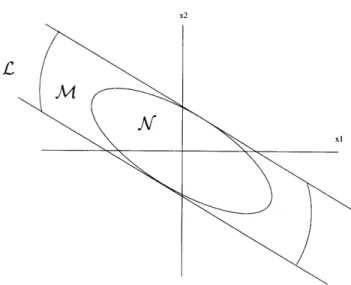
Figure 3-1: The Sets C, M, and N"

where ca = 1/ max(diag(KP-1_K T _{)) is found by solving a simple optimization}

prob-lem. The sets £(K), MA(K), and

N

order system.

We can now use this knowledge to build a globally stabilizing bounded control. The basic idea is quite straight forward. It is to use low gains, corresponding to a large

M(K), when far from the equilibrium to avoid control saturation, and progressively

higher gains, corresponding to a smaller and smaller M(K), as the state becomes closer to the equilibrium. This idea follows quite intuitively from noting that the control u is a gain-state product Kx. For each K we can use an invariant ellipsoidal

approximation to the region M (K) to guarantee stability and control boundedness.

In other words the gain is scheduled to avoid saturation at all times. The challenge arises in finding a computationally efficient manner in which to compute K and P for the best possible performance. The method of choice in this exposition is the Linear Quadratic Regulator (LQR). There are numerous reasons for this choice.

* Solution is optimal with respect to a meaningful quadratic cost. * Multiloop control design.

. Excellent gain and phase margins.

* Production of a natural Lyapunov function.

The standard LQR problem is to minimize the quadratic performance index

J = (xTQx + uTRu)dt. _(3.3)

0

The solution to this problem is found in the matrix P of the Algebraic Riccati Equa-tion (ARE)

ATP + PA - PBR-BTP + Q = 0, (3.4)

and the associated gain matrix, K = -R-BTP. The properties of the solution

matrix P depend, in general, on the assumptions made about the dynamic system involved. We will be interested in the case where the system is ANCBC, and the properties of the Riccati equation are yielded by the following lemma.

Lemma 3.1 Let Assumptions 2.1 and 2.2 hold. Take R = rIm, where r

e

there exists a unique positive definite solution P(r) to the ARE with the following properties

1. The matrix A + BK is stable or Hurwitz.

2. P(r) is continuously differentiable with respect to r and dP(r) _{> 0, for any r.}

dr

3. lim P(r) = 0.

r--0

4. P(r) is an analytic function of r.

5. The function V = xTP(r)x, for any r, is a Lyapunov function for the system (2.18) with state feedback u = Kx.

Proof: The proof of items 1-3 follows directly from Lemma 3.1 and Remark

computation the function V = xTp(r)x satisfies the conditions of Theorem 2.1 for any r.

3.1

Position Constraints

The methodology presented in the previous section can be used to solve the NSFP problem by means of the following theorem. An almost identical result was first proven by Wredenhagen and Belanger [81]. The result presented here was first

re-ported in [53].

Theorem 3.1 Let Assumptions 2.1 and 2.2 hold. Take R = rIm, where r E R+.

Then the control

BTP(r)

U -- X1

r

with P(r) the solution to (3.4), and for any time t

r(x(t)) = min r : x(t)

c

₍

(3.5)

In order to simplify the proof we need to establish some important properties of a(r) that have not been discussed previously. First note that a(r) can also be written as

a(r) = 1/ max (bTP(r)bi/r2_{), (3.6)}

i=l,...,m

where bi is the ith column of the B matrix.

Lemma 3.2 ac(r) is a continuous function of r. Furthermore, let i* be the column

number that achieves the maximum in (3.6) (note that it need not be unique). Then either the maximum is achieved by one value of i*, for all r, or the value of i* changes only a finite number of times.

Proof: The proof is in two parts.

a) a is continuous: First note that P(r) is a continuous and unique function of r from Lemma 3.1. Then a(r) is continuous by virtue of the fact that the maximum function is continuous and a composition of continuous functions is continuous [59].

b) finite switchings: Let r take values on the nonempty bounded interval [ri r2],

where r2 > r1 > 0. Consider two columns of the B matrix, bi and bj. Assume

that bTP(r)bi = bT P(r)bj for an infinite number of values of r

e

the Bolzano-Weierstrass theorem there exists a limit point r*. Now, because P(r) is an analytic function of r from Lemma 3.1, Theorem 10.8 in [66] tells us that

bTp(r)bi = bTP(r)bj over the whole interval r

c

two values an infinite number of times the maximum is achieved by both bi and bj over the whole interval of r. This can be extended to any arbitrarily large nonempty bounded interval of r and any number of possible maximizers.

Clearly, the only other possibility is that the value of i* switches only a finite number of times, and thus the lemma is proven.

We are now ready to prove Theorem 3.1.

Proof: [Theorem 3.1] The proof consists of three parts. Showing that there

exists an invariant ellipsoid for each value of r, that these ellipsoids are nested, and that the outer ellipsoid can be made arbitrarily large.

a) Invariance: From item 5 of Lemma 3.1 we have that V = xTP(r)x is a Lyapunov

function for any r. Clearly, we can use Theorem 2.2 to show that the ellipsoid

(P(r), a(r)) is invariant and any trajectory that starts there will not violate the

constraints because of the scaling (3.5).

b) Nesting: A necessary and sufficient condition for nesting is ([81, 53])

dP(r) < 0 _(3.7)

dr

-where

P(r)

Taking the derivative of (3.4) with respect to r and collecting terms gives

PBBTP

AdP + dPAt + r2 dr = 0, _(3.9)

where A = A BBTP(r . Now consider the case where there is one maximizer b of

r

the function (3.6). Taking the derivative of P(r) with respect to r yields

S dP bTdPbP P

dP(r) d(bPb) r2 + 2P 2(bTPb) H dr. _(3.10)

From (3.9) we can write

dP(r) ATTPBBTP

dr o r eAcldT, (3.11)

and from (3.4) P satisfies

00

P

(r) =

CC

Substituting (3.11) and (3.12) into (3.10) we eventually obtain (after some manipu-lation) dP(r) [o) eATrQeAcldT p

+bT

Thus the condition (3.7) is satisfied for the case of one maximizer b. Now, P5(r) is a continuous function of r, that has a decreasing derivative over a finite number of intervals of r from Lemma 3.2. Thus P(r) is a decreasing function of r over any interval

c) Global Stability: Under Assumption 2.1 it clearly takes only an infinitesimally small gain to asymptotically stabilize the system. Thus the gain vector K(r) can be made arbitrarily small and global stability can always be guaranteed [81].

Thus for any value of x0 there exists a bounded control via the value of r defined by the ellipsoid 8(P(r), ao(r)) such that the trajectory will always move in towards the

next inner ellipsoid. Furthermore, it is important to note that although the function

V = xTP(r)x is a quadratic Lyapunov function for each particular value of r, the

function V(r) = xTP(r)x over all r is a non-quadratic Lyapunov function. Indeed,

the function V(r) can be used to establish global asymptotic stability.

U

This result deserves several comments. For each value of r we arrive at a matrix

P(r), and thus a gain K(r). The scaling (3.5) provides us with the best ellipsoidal

approximation to the region M(K), in terms of P(r). The proof of stability in Theorem 3.1 hinges on showing that the set of ellipsoids

Q = {$(P(r), a(r)) :r E R+} (3.14)

is nested, i.e.,

£(F(r1),a(r1)) C 8(P(r2), a(r 2)) for any ri < r2.

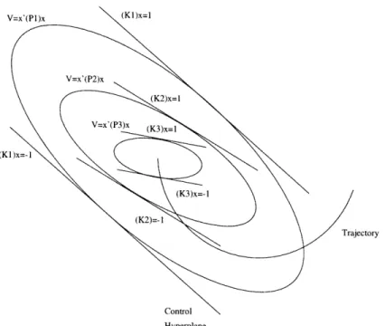
Indeed, this is brought about by scaling (3.5). This nesting property binds the con-struction together. Each ellipsoid defines an invariant region under which the controls are guaranteed not to saturate. Furthermore, the system state will always move to-wards the next inner ellipsoid guaranteeing a stable system and allowing the controller gain to be steadily increased to improve performance. A schematic of this is shown in Fig. 3-2.

Although this construction is continuous in the parameter r, in practice, only a finite number of ellipsoids are used. The most straightforward and efficient way to do this is to choose a geometric sequence

R=- {r R+:r= rrmax/A , i E {0,...,N}}, (3.15)

where rmax E R+, N E 1+, (A - 1) E R+. The value of rmax must be chosen such

that all expected initial conditions will be in the set Q generated by R. The other two parameters N and A can be chosen, as desired, to obtain an even distribution of

V=x'(Pl)x

(K1)x=-1

Trajectory

Control

Hyperplane

Figure 3-2: Nested Ellipsoids ellipsoids.

Also, note that the control constraints (2.21) have been normalized to unity as dis-cussed in Section 2.3. This is the most significant difference between the construction of Theorem 3.1 and the results in [81]. The Piecewise-linear Linear Quadratic (PLC) control law developed in [81] uses an iteration function to adjust the elements of the

R matrix so that tangency between each ellipsoid and the control planes P(k (r)) is

guaranteed. By tangency we mean that the set P(kT (r))n (P(r), a(r)) is non-empty for any r and i.

Instead of choosing the values for r, the PLC law is constructed by choosing values of the parameter p for S(P, p). The control weighting matrix is chosen as

R = diag(e) = diag( 1,... . 2), -i > 0. Then for a given p, c is chosen such that

Iui

where bi is the ith column of the B matrix. It is shown in [81] that for any initial value of E the iteration function

n+1

where

4)(E)

¢ (r,..,

I

n(O)]T,

and

l =-bTPb,

converges to a unique value. An initial value po is selected to contain the initial conditions and successive ellipsoids are generated by a reduction factor Ap. However, this does result in an added computational burden because for each ellipsoid in the set a series of iterations must be performed. A simple yet effective way around all of this is to use the gain margin of the LQR ([63]) to guarantee tangency. In particular each gain vector can be scaled as

() = k (r) a(r)ki(r)P-1 (r)kT (r) if 1

ki(r) > -ki()

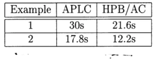
which is the gain margin of the LQR. Indeed, this is always the case since the control gains are always increased by this scaling. In a number of simulations this construc-tion always resulted in nearly identical overall performance to the iteraconstruc-tion funcconstruc-tion method. For example, a comparison was performed between the PLC and the High Performance Bounded (HPB) method presented here for the PUMA 560 Robot ex-ample given in [81]. In that exex-ample the authors use the state energy

J = xTQx dt 0O

as a performance measure. With the PLC simulation parameters

N = 100, Po = 1043, Ap - .94

the control law achieved a value of JPLc = 324. A controller was constructed for this

example using the method described here with the parameters

N - 100, rmax 9000, A- 1.05.

The state energy was calculated as JHPB = 334 indicating a difference of

approxi-mately 3%.

3.1.1

An Academic Example

In this section we will present a simple example that illustrates the High Performance Bounded (HPB) method described above. Consider the double integrator system

0 1 0

A = B = . (3.16)

0 0 1

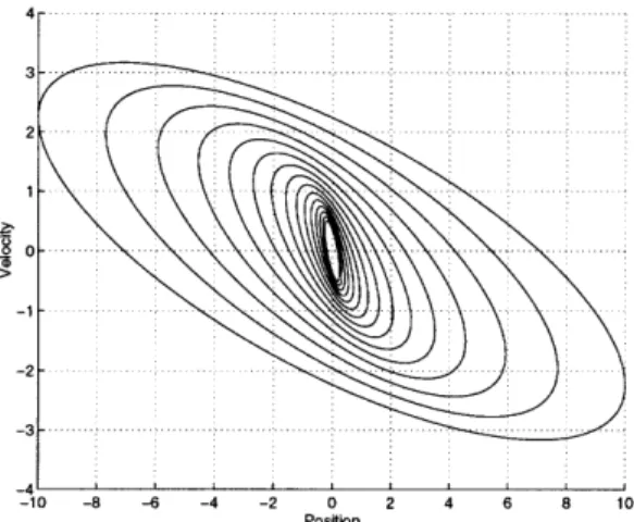
The control law construction parameters in (3.15) were chosen as

rmax =100, A = 1.3, N = 100,

and the state weighting matrix was chosen as

Q = diag(1, 0).

The ellipsoids are shown in Fig. 3-3 and the system states and control are shown for

an initial condition of xo = [2 0]T in Fig. 3-4.

Note that the control effort is highly nonlinear when the state approaches the origin. The proximity to the origin allows for a high gain to be used resulting in a sharp convergence, with no overshoot. Also, the control is inherently rough due to the

Figure 3-3: Nested Ellipsoids for Double Integrator Time (sec) 0 V _--0.2 \ 0 2 ~- -.4 VI -0.6 -0 .8 ... .. .... ...:... 0 0.5 1 1.5 2 Position

switchings that occur when the trajectory crosses from one ellipsoid to another. This can be reduced by adding more ellipsoids, but this results in a higher computation and storage burden. Indeed, the choice of the number of ellipsoids to use is somewhat subjective. As noted in [81] most of the advantage of the controller can be achieved through as few as five ellipsoids. It was also shown in [82] that an interpolation function can be used to smooth the control. The interpolation function has the additional advantage that it can be used to reduce the number of ellipsoids by taking a more spread out distribution, i.e., an increased A.

For a second order system such as this it is even possible to analytically compute the solution to the Riccati equation and the resulting gain as,

P (r) = '2r1/ I V V/-2P3 / 4 K (r) - [r-1_/2 _v/ - _{1/4] (3.17)} v/2r - I v2-3/4T

P(r)

[

3.1.2

Limit Properties of Invariant Ellipsoids

An important consideration for the control methodology, from the standpoint of sta-bility, is the limit properties of Q. In the proof of Theorem 3.1 we have seen that global stability is guaranteed because the ellipsoids can be made arbitrarily large, i.e.,

lim S(P(r), a (r)) = R' .

T -- OO

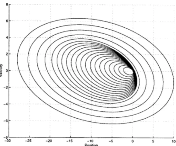
This is provided by Assumption 2.1 that guarantees the system is globally control-lable. For unstable systems it is not possible to obtain global stability and the outer most ellipsoid will approach a limiting shape, as in Fig. 3-5 for an unstable pendulum. In the converse direction it is important that as r -± 0 the ellipsoids, corresponding to the increasingly aggressive gains K(r), uniformly decrease to the origin. If this were not the situation one could imagine a case where the gains become increasingly large and the state is not driven to the equilibrium. The following lemma asserts a

3-. 3-. 3-.. . . . . .... .... .. . . ... .. . ... . . ...

-2

-2 -1.5 -1 -0.5 0 0.5 1 1.5 2

Angular Position

Figure 3-5: Open Loop Unstable System

condition under which the ellipsoids must uniformly collapse to the equilibrium.

Lemma 3.3 Let Assumption 2.1 and 2.2 hold. If the state weighting matrix, Q,

is positive definite then the largest diameter, in the standard Euclidian sense, of (P(r),a(r)) approaches zero as r approaches zero.

Proof: By Contradiction.

Assume that Q > 0 and the largest diameter, in the Euclidian sense, of S(P(r), a(r))

does not approach zero as r goes to zero. Then it follows that there exists an x* such that fx*| > 0 and

X*

n

Indeed, consider any infinite sequence oc > r, > r2 > ... rn > ... , where limn--oo rn=

0. Then, by the hypothesis, there exists a sequence x1,X2,..---,Xn,... such that

x, c S(P(r),a(ri)), and |xl > m = 0 (1 = 1,...,n,...). Now, the first

el-lipsoid S(P(r),a(r1)) covers a bounded domain because P(ri) > 0 and oc > rl.

Thus, the set of all xz is bounded above and below, that is there exists M and m

such that, M > { 11,XI,X2 - -, X. n , .} > m = 0. It follows from the