Modélisation mathématique pour la simulation des processus agrégatifs

Modélisation mathématique pour la simulation des

processus agrégatifs

Mathematical modeling for the simulation of aggregative processes

1

A.T.I. Rome, Italy, [email protected] 2

Dipartimento di Ingegneria Industriale, University of Florence, [email protected]

RÉSUMÉ. En introduisant le concept statistique d'entropie d'allocation et en combinant des éléments théoriques mé-diés par la thermodynamique statistique et la théorie de l'information, on arrive à une expression markovienne de l'en-tropie absolue d'un mélange gazeux. Dans cette expression, la qualité du gaz est représentée par l'enl'en-tropie d'une source de Markov décrivant le mélange en termes de concentrations de chaque type de particule impliquée. La struc-ture particulière de cette formule ouvre la voie à la construction d'un modèle théorique pour l'étude des phénomènes agrégatifs codifiés. Les concepts de “particule élémentaire idéale” et de '”agrégat ideal” sont d'abord définis; puis une réaction particulière est proposée comme processus d'agrégation hypothétique. Ensuite, des relations décrivant la thermodynamique du processus de formation de structures même très complexes sont obtenues en conséquence des règles de combinaison. Ceux-ci sont exprimés en termes de “facteur de codage”, une sorte de taux de nécessité sur une base aléatoire. En effet, en raison de l'expression markovienne de l'entropie absolue, le modèle élaboré permet l'utilisation de codes d'agrégation plus ou moins forts de manière à simuler des environnements totalement dominés par le hasard ou totalement déterministes, en passant avec continuité par tous les intermédiaires possibles situations. Enfin, la structure du modèle permet de distinguer entre les processus qui se développent en conséquence de ten-dences agrégatives implicites dans le système lui-même (processus autopoïétiques) et les processus qui se dévelop-pent en conséquence de l'action d'ordonnancement d'entités extérieures au système (processus hétéropoïétiques).

ABSTRACT. Through the use of the statistical concept of allocation entropy and by combining theoretical elements

derived from statistical thermodynamics and information theory, a Markovian expression of the absolute entropy of a gaseous mixture is achieved. In the formula, the quality of the gas is represented by the entropy of a Markov source describing the mixture in terms of concentrations of single types of particles involved. The special structure of this for-mula opens the way for the construction of a theoretical model for the study of codified aggregative phenomena. The concepts of “ideal elementary particle” and “ideal aggregate” are firstly defined and then a particular reaction is propo-sed as a hypothetical aggregative process. Then, relations that describe the thermodynamics of the formation process of even very complex structures are obtained as a consequence of the combination rules. These are expressed in terms of “coding factor”, a kind of necessity rate on a random basis. In fact, thanks to the use of the Markovian ex-pression of absolute entropy, the elaborated model allows the use of more or less stringent aggregation codes so as to simulate environments totally dominated by chance or totally deterministic, passing with continuity through all possible intermediate situations. Finally, the structure of the model permits to distinguish between processes that develop as a consequence of aggregative inclinations implicit in the system itself (autopoietic processes) and processes that deve-lop as a consequence of the ordering action of entities outside the system (heteropoietic processes).

MOTS-CLÉS.Entropie, modélisation mathématique, processus agrégatifs, sources de Markov,hasard et nécessité. KEYWORDS.Entropy, Mathematical modeling, Aggregative processes, Markov sources, Chance and necessity.

1. The Markovian expression of the absolute entropy

Let a system of particles belonging to distinguishable groups be given. We call absolute

population descriptor the vector [ ] [ ] of the order whose components represent the number of indistinguishable particles in each group so that

∑ [1]

If we indicate with the probability that the generic particle belongs to group , then we define probabilistic population descriptor or more simply population descriptor the vector

[ ] [ ] [2]

of order . Its components represent the probability that, following a random choice, the generic particle of the system belongs to a certain group. Let us now suppose that the particles are contained in a volume fractionated into identical elementary cells, called allocation cells, having volume such that

[3]

If , then the number of the ways particles can occupy allocation cells is given by1

∏ [4]

We then define the following quantity as allocation entropy of the particle system:

∑ [5]

where constant remains for now undefined. Recalling Stirling's formula2 and taking into account [1], [2] and [3], [5] can be developed as follows:

∑ ( ) ∑ ( ) [ ( ) ∑ ] that is, * + [6]

where the quantity

∑ [7]

can be defined as entropy of the population descriptor being the descriptor [ ] comparable to a no-memory Markov source3.

Statistical thermodynamics provides a simple formula for calculating the absolute entropy of a gas consisting of linear molecules4 (typically diatomic molecules, but not only):

1 _{See [Ref.1], Chapter 10, paragraph 2.}

2

The Stirling’s formula ( ) ( ) approximates the logarithm of a factorial: the precision is the more accurate the greater the value of n.

3

See [Ref.5]. 4

[ (

)

] [Joule/°Kmole] [8]

where:

- is the Boltzmann constant (=1,380649 10-23

Joule/°K) - is the absolute temperature in °K

- is the molecular mass in Kg

- is the Plank constant (= 6,62607 10-34 _{Joule sec)}

- is the molecular symmetry number (= 1 for asymmetric molecules and = 2 for symmetric molecules)

-

is the rotational characteristic temperature in °K where is the molecular

baricentric moment of inertia in Kgm2 ( = molecular length in m and = reduced mass in Kg).

Formula [8] does not take into account the internal vibrational phenomena of the molecule (i.e. a rigid molecular structure is assumed) but under standard temperature and pressure conditions it still provides values in excellent agreement with the results of the calorimetric measurements, as will be shown below. The formula highlights that two contributions to total entropy can be clearly distinguished: a thermal contribution that depends on the absolute gas temperature (and therefore on the more or less wide maxwellian distribution of molecular velocities) and a geometric-inertial contribution that depends on the spatial distribution of the particles (through the ratio) and on their inertial characteristics ( , and ). It is easy to demonstrate that the latter contribution can be expressed as a function of the previously defined allocation entropy, if and a volume is assumed for the allocation cell depending on the inertial characteristics of the molecule according to the following relation:

( ) ( √ ) [m 3 ] [9]

In fact, by matching [6] (with and therefore ) and the second two terms of [8] we obtain

* + [ ( ) ] hence ( )

and consequently [9]. It should be noted that the greater the translational and rotational inertia of the molecule, the smaller the volume of the allocation cell. This is because the increase in inertial pa-rameters implies an increase in energy levels accessible to the molecule and therefore an increase in the number of micro-states physically possible. The higher splitting of the reference volume is there-fore functional to the achievement of a higher value of entropy as a macroscopic state function. Therefore, the expression of the entropy of a homogeneous gas ( ) made up of linear molecules takes the form:

* + [10]

Evidently, in the general case where , if we indicate with the entropy of the i-th group of particles, according to [10] and recalling [1], we have:

∑ ∑ * + [11]

where is the volume of the allocation cell pertaining to the molecules of the i-th group according to [9]. It can be demonstrated that the calculation of the entropy of a mixture of distinguishable groups of indistinguishable particles implies the choice of a single volume for the allocation cell according to the following relation:

∏ ( ) [12]

In fact, by developing the summation in [11] (which represents the geometric-inertial contribution to total entropy) and recalling [7], we obtain:

∑ ∑ ∑ ∑ ∑ ∑ ∑ [ ∑ ]

From the comparison of this expression with the second term of [6] (where is placed) we immediately obtain that, for , it must be

∑

and consequently [12].

In conclusion, established and therefore ( , the Avogadro number; Joule/°Kmole, the gas constant) the expression of the absolute molar entropy of a mixture in the gaseous state of different substances characterized by linear molecules, takes the form:

* + [13]

where the volume of the allocation cell is given by [12] and in this formula each is given by [9]. In [13] both and depend on the number of species varieties and on the relative composition of the mixture [ ]. For the presence, in the entropy formula, of the population descriptor, we call this expression of absolute entropy Markovian.

As an example, calculations of standard molar entropy were performed - for a gas with a symmetrical diatomic molecule ( ),

- for a gas with an asymmetrical diatomic molecule ( ) - for a mixture of the two ( ).

Figure1. Comparison between the experimental values of standard molar entropy and the values calculated by means of the Markovian expression of entropy

Results obtained using [13] by calculating

- volume of the allocation cell in the first two cases

- volume of the allocation cell and descriptor entropy in the third case

are obviously identical to those obtained using [8] and in excellent agreement with the results of the calorimetric measurements5 (see Fig.1). It should also be noted that sizes of allocation cells are al-ways much smaller than the average volume6 at disposal of a single molecule under standard condi-tions (4,063 10-26 m3), thus verifying the validity of [4].

2. The ideal elementary particle

The fundamental brick of the proposed model is the ideal elementary particle (IdEP) which, go-ing beyond the physical concept of atom or molecule, concentrates the inertial characteristics in a homogeneous material segment. Each IdEP is therefore exhaustively defined by:

- the mass - the length

- the colour that makes the particle distinguishable although they have the same inertial charac-teristics.

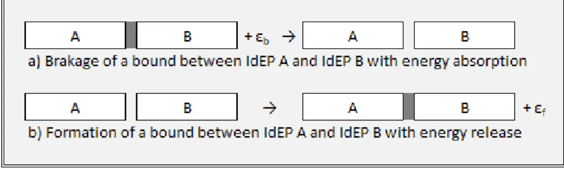
It is also assumed that an IdEP under standard temperature and pressure conditions can exist in two states: a free state in which the particle stays alone or a bound state where two or more par-ticles are joined together. In general a bound IdEP can be

- part of a reactant from which it can dissociate, absorbing from the environment the energy necessary to break the bond (Fig.2/a)

5

See [Ref.4]

6 _{it should be noted that the volume of the allocation cell is not necessarily such that it accommodates the entire particle.} Ra-ther, it represents the tolerance with which the position of its barycenter in space is set.

- part of a reaction product formed with other particles: in this case the energy of formation is dispersed in the environment (Fig.2/b).

Figure 2. Diagram of IdEPs and of their chemical combinations

Due to the one-dimensional nature of the particle, the volume of the allocation cell of a gas formed by IdEPs of a single species can be calculated by [9]. Being in fact

and defined as follows the allocation inertia which aggregates the inertial characteristics of the IdEP: √ we immediately obtain: ( _{) [14]}

3. The ideal aggregate

It is assumed that IdEPs just defined, thanks to a succession of couplings, can give rise only to one-dimensional products that we will call ideal linear aggregates (IdLA). In the particular case in which aggregating IdEPs have the same inertial characteristics (possibly differing only in colours), if we indicate with the number of particles that make up the generic IdLA, its total mass , its barycentric moment of inertia , its rotational temperature and the volume of its allocation cell can be immediately calculated as follows

( ) [15] ( ) ( ) [16] ( ) [17] ( ) ( ) _{( )} [18]

4. The aggregating reaction

Let an initial system be given in the gaseous state under certain conditions of temperature and pressure, consisting of a mole of reactants thus formed:

- α fraction of giver compounds: we suppose that the generic compound is formed by only two IdEPs and that it is therefore an IdLA of order ; we will refer to the first particle with and we will call it grey particle; we will refer to the second particle with and we will call it active primary particle; we also suppose that the grey particles are all the same while the active primary particles, even if they share among themselves and with the grey particles the same inertial characteristics, have different colours: so many different types of giver compounds are given

- fraction ( ) of passive primary particles. It is assumed that these particles, which we will refer to as , have the same inertial characteristics and that these characteristics are also identical to those of active and gray particles; nevertheless they can differ in colours (where, in general, ).

It is assumed that the reactants described above, as a consequence of the giver compounds dissociation, give rise to a substitution reaction. As a result, particles remain isolated while and particles aggregate with the only condition that, regardless of the IdLA’s length, the passive particles are always and only at the end of the sequence. In essence, the aggregating reaction just described can be formally represented as follows:

( ) ∑ [19]

where:

- is the length of the generic aggregate

- is the maximum value of to be taken into account7

- is the generic IdLA of length , consisting of active particles and a passive par-ticle in sequence closure; with we refer to the passive primary parpar-ticles that remain in the free state even after the completion of the aggregating reaction

- is the molar fraction of the IdLA of length as a consequence of a complete reaction:

these values evidently depend on the aggregation rules

- the sign ↔ between reactants and products indicates the possibility that, depending on the bonding energies involved, the reaction can find the balance with non-zero reactant concen-trations.

Since the aggregates (including those of order ) have one and only one inactive primary particle, the stoichiometric balance of [19] concerning particles immediately leads to the following

∑ ( ) [20]

Therefore, if the initial system consists of one mole of reactants, the final system also consists of one mole of products. Finally, note that it is also possible to calculate the average length of the IdLA’s set: as the total number of primary particles involved in the formation of the aggregates is

7 _{The value of depends on the number of active particles (and therefore on the quantity of giver compounds) present in the} system and on the aggregation logic: in the case of random aggregation for 0,1 the aggregates with represent just 0,01% of the population while to obtain the same percentage with 0,95 we must assume .

, the number of IdLAs produced by the complete reaction of one mole of reactants is, for [20], ( ) . Consequently, the (weighed) average of the lengths is always

( ) ( ) [21]

regardless of the aggregative rules8.

5. General relations of aggregation: entropy

We assume that the initial system consists only of reactants. If we indicate the extent of reaction with , we can define as follows the molar fraction of each species as the reaction progresses:

( ) ( ) [22/a]

( ) ( )( ) [22/b]

( ) consequently from [20]: ∑ ( ) ( ) [22/c]

( ) [22/d]

The entropy of the gaseous mixture as a function of the extent of reaction is given by the sum of the entropies of the single species instant by instant, that is:

( ) ( ) ( ) ( ) ( ) [23]

where, being the number of particles in equal to for any value of , ( ) ( )( ) ( )( ) * ( )( ) ( ) + [23/a] ( ) ( ) ( ) * _{( )} ( ) + [23/b] ( ) * ( ) + [23/c] ( ) ( ) ( ) * _{( )} ( ) + [23/d]

The IdLA subscript refers to the aggregate complex (with ranging from 1 to ). All the quantities that appear in the first three relations are immediately calculable according to already obtained formulas: in particular, according to [9] we have

[24/a] [24/b] [24/c] ( ) [24/d] and according to [7] ∑ ∑

8 _{If it is assumed, as permissible, that relative ratios among single aggregates do not change in the course of reaction. Then [21]} also applies to any value of (i.e. ratios do not depend on the extent of reaction).

It should be noted that the entropy of the descriptor [ ] (related to passive primary particles) and the entropy of the descriptor [ ] (related to giver compounds i.e. active primary particles) are limited by the conditions of equiprobability:

∑ ∑ Consequently, in general: [25/a] [25/b] [25/c]

where and indicate how far each descriptor is from a uniform distribution: we will refer to them as disequilibrium factors.9

The volume of the allocation cell and the entropy of the aggregates descriptor are less immediately calculated. A first step in computing the first one can be done considering that, from the inertial point of view, IdLAs of the same length have the same behaviour independently of the sequence of colours: in [12], the generic probability 10 _{can therefore be replaced by the probability}

that the generic IdLA has the length . Consequently:

∏ ( ) [26/a]

∑ [26/b]

However, the values of (and therefore the value of ) remain unspecified as long as no aggregation rule is defined. To achieve this goal, a tool generating a descriptor of the aggregate population11 is required.

For the same reason the calculation of entropy is a priori not possible. So, let’s entrust the generation of the aggregates population (and therefore its description) to a sequencer which, operating as a Markov source, proposes a certain sequence of primary particles in accordance with a predetermined rule: in this way we obtain strings of different lengths formed by variously colored sequences of active particles with a single passive particle at the end. If the sequencer operates without memory, then its entropy (no-memory entropy) can be obtained as follows:

∑ ( ) ( ) ∑ 9

Disequilibrium factors are less rich in information than the descriptors producing and as the same disequilibrium factor

can be generated by different descriptors, but this does not affect entropy determination as a macroscopic state function. 10 _{In general: ∑}

11 _{In this case the number of aggregates is, potentially, very high due to colours that must be taken into account. Note also that}

can be considered independent from only if we admit that are independent in the same way, which implies the

as-sumption that the descriptor of the aggregates (i.e. their relative distribution) does not change during the reaction (see also note 7).

( ) ∑ ( ) ( ) ∑ ( ) ( ) ( ) that is ( ) [27] where ( ) ( ) [28]

On the other hand, if the sequencer operates as a Markov source with memory, then its entropy

(with-memory entropy) is necessarily:

( ) [29]

Well, we can assume that the following simple relationship12 links the entropy of the aggregates descriptor and the entropy of the sequencer (with or without memory):

[30]

Consequently:

in the case of no-memory sequencer in the case of with-memory sequencer

In general, we can then write:

( ) * + [31]

where the coefficient , called the coding factor, has a value ranging from 0 to 1. The limit case in which implies that the sequencer operates as a Markov source without memory, while in the other limit case in which , the entropy of the aggregates descriptor is equal to zero, as any uncertainty in the formation of the aggregates disappears. In this second case the aggregates population can be formed only by the sequence of a limited number of aggregates (at the most, only one) produced by the sequencer ad infinitum. This extreme mode of assembly is called compulsory

assembly.

We have thus given manageable expressions to (through the probabilistic distribution ) and to (through the coding factor ). Note that both and derive directly from the sequencer (to be defined each time) as a necessary consequence of the way it works. Note also that

12

Relationship [30] can be demonstrated in closed form in the case of equiprobability of [ ]and [ ] and no-memory sequenc-er. Otherwise a general demonstration is not available at present even if a large number of numerical simulations confirm its va-lidity.

the relationship between these quantities is clearly only univocal: from a sequencer, only one value of probabilistic distribution (and hence of ) and only one value of the coding factor (and hence of ) can be derived while a given distribution [ ] as well as a given coding factor can be generated by different sequencers. In fact, the sequencer contains as much information as possible about the aggregates population while [ ] and constitute synthetic macro-information, even if sufficient to determine entropy as a statistical function. As a result of this, values of [ ] and and can be assumed, to a certain extent, independently of each other, as we shall see later.

At this point we can also derive the expression for the reaction entropy as: ( ) ( )

where is the reaction extent at which a dynamic equilibrium is established between reactants and products ( for complete reactions and for incomplete reactions). As far as expressions of , , e are concerned, from [23] we obtain:

( ) ( ) ( ) [ ( ) ( ) ] ( )( ) ( ) ( ) ( ) [ ( ) ] ( ) ( ) ( ) ( ) [ ( ) ] ( ) ( ) ( ) [ ( ) ( ) ] After a few steps we get:

* ( )

( )++ ( )[ ( ) ( ) ]

[ ( ) ( ) ] and by means of [25] and [31]:

* ( )

( )++ ( )[ ( ) ( ) ]

[ ( ) ( ) ] ( ) Finally, using [24/d] and [26/b] we obtain:

[ ( ) ( )] ( ) ( ) [ ∑ ] [ ]

This relation clearly shows the dependence of reaction entropy on [ ] and on . On the other hand, it also shows how reaction entropy is independent from the inertial characteristics of IdEPs. Moreover, all other conditions being equal:

- the coding factor (which appears three times in the formula) gives a negative contribution to : high values of (at the limit ) tend to reduce reaction entropy by creating more and more ordered final systems

- the average length of the aggregates gives a positive contribution to . The more the se-quencer produces long aggregates (and therefore also greater mass, regardless of the specific values of and , in itself irrelevant), the more the reaction entropy increases. In fact, the larger the IdLAs size, the smaller the volume of the allocation cell with a consequent increase in entropy, in compliance with [13]

- the number of colours and and disequilibrium factors and play their roles through the aggregated parameters and , i.e. through the entropies of the primary parti-cles descriptors. Both the entropies give a negative contribution to which means that, all other conditions being equal, in an initially more disordered system the aggregation brings more order than in an initially more ordered system.

6. General relations of aggregation: enthalpy, free energy and affinity

Let us indicate with:

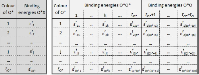
- (with ranging from 1 to ) the energy stored in each of the different types of bond in the giver compounds

- (with ranging from 1 to and ranging from 1 to ) the energy stored in each of the ( ) different types of and bonds within the IdLAs

- the overall number of type bonds present in the initial system

- the overall number of and type bonds present in the final system. To be clearer:

- in Fig.3 matrices [ ] and [ ] of the elementary energies associated with breaking and forming bonds respectively are schematically represented

- in Fig.4 matrices [ ] and [ ] of broken and formed bonds as a result of the aggregative pro-cess are represented.

We can then define as follows, the energy that must be supplied to a mole of giver compounds to break the internal bonds and the energy released by a mole of aggregates as a result of the new bonds formation: ∑ [33/a] ∑ ∑( ) [33/b]

Figure 3.Binding energies

Figure 4. Number of bonds

The former provides a positive contribution to the enthalpy of the system, while the latter provides a negative one. The enthalpy of the gas mixture being reacted will therefore be given by the sum of the following contributions:

( ) ( )( ) [34/a] ( ) ( ) [34/b] ( ) [34/c] ( ) ( ) [34/d] and hence: ( ) ( ) ( ) ( ) ( ) ( ) [35]

where is the molar energetic balance.

The reaction enthalpy is also immediately obtained from [35]:

where is, as said above, the extent of reaction at the equilibrium.

So defined entropy and enthalpy of the mixture as well reaction entropy and reaction enthalpy, the values of the Gibbs free energy ( ) and of the reaction free energy can be easily calculated:

( ) ( ) ( ) [37]

[38]

Finally, from [38] we obtain the affinity ( ): ( ) ( ) ( ) [39] where, by derivation of [23]’s, ( ) * ( )( ) ( ) + [39/a] * ( ) ( ) + [39/b] * ( ) + [39/c] ( ) * ( ) ( ) + [39/d]

Relationship [39] verifies the fact that the reaction proceeds until ; then, when the extent of reaction reaches the equilibrium value so that ( ) , the reaction stops.

It must be noticed that the relations drawn in this paragraph as well as in the previous one disregard the rules of aggregation: therefore, a kind of general validity can be attributed to them, even within the limits of the hypotheses made.

7. Autopoiesis and heteropoiesis

The theoretical development of the model proposed in paragraphs 5 and 6 shows that, once the initial system has been defined in terms of

a) concentration of giver compounds

b) descriptor [ ] ( ) of the particles population that makes the calculation of (i.e. of ) possible

c) descriptor [ ] ( ) of the population that makes the calculation of (i.e. of ) and the calculation of the matrix [ ] possible

d) matrix [ ] ( ) of elementary energies associated with bonds that, in combination with matrix [ ], makes the calculation of the molar energy possible e) matrix [ ] ( and ) of elementary energies associated with

and bonds

it is then necessary to define the rules of the aggregative process (that means to define a sequencer) in order to describe in detail the course of the reaction and achieve the final thermodynamic state of the system. In fact, only the knowledge of the sequencer’s mode of operation allows us to calculate

f) entropy of the IdLA descriptor, that is the coding factor , through [31] g) matrix [ ], computing the IdLAs internal bonds

and consequently:

h) molar energy through (33/b) and hence molar energy balance in combination with i) extent of reaction by imposing zero value to affinity expressed by [39].

With all these elements, relations [32], [36] and [38] will enable the calculation of reaction entropy, reaction enthalpy and reaction free reaction respectively.

It is now appropriate to distinguish two possible ways of making our model work, when it simulates the aggregative processes that actually occur in nature. A first mode of operation can describe those processes that are exclusively guided by chemical-physical characteristics of the reactants while a second mode can be representative of the more complex reality of those processes which are influenced by external agents, not strictly belonging to the system. With the first case we intend to fall within the field of chemical reactions (also organic, catalyzed or not) while in the second case we intend to include those phenomena of complexity construction that are more typical of biochemistry. Within our model we then define:

- autopoietic , that aggregative mode in which the formation of reaction products is deter-mined, for quality and quantity, exclusively by the properties of the system: the sequencer will then behave in a way univocally established by conditions a), b), c), d), e) above

- heteropoietic , that aggregative mode in which the reaction is controlled by factors extrane-ous to the system: in this case the sequencer will impose its own aggregative rule, aimed at forcing the basic autopoietic behaviour in a more or less accentuated way.

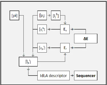
In more detail, the autopoietic aggregation can be interpreted in the following way (see Fig.5). Matrix [ ] comes out as a necessary consequence of the chemical characteristics of the system itself. In the same way, molar energy and molar energy balance must be considered univocally determined as implicit in the system. But matrix [ ] is also provided by the IdLA descriptor, which in turn is univocally determined by the sequencer. That means that the sequencer cannot argue with the relationship of necessity that links the system characteristics to its energetic evolution. It follows that a relation must also exist between system characteristics and the sequencer. Moving from the microscopic to the macroscopic level, there must exist some constraint linking molar energy balance and sequencer’s entropy coding factor .

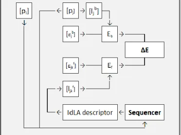
Figure 6. Logical chart of heteropoietic aggregation

In the case of heteropoietic aggregation, the flow chart in Fig.6 applies instead. In this case the matrix [ ] is determined exclusively by the sequencer which, with the only limit of respecting descriptors [ ] and [ ], imposes its own coupling code forcing the aggregates construction regardless of any autopoietic guidance. Therefore, the dissipated molar energy and consequently the value of are conditioned. Also in this case a relationship must exist between the energy balance and the sequencer entropy (i.e. the coding factor ). The fundamental difference between the two schemes lies in the different roles played by matrix [ ]: in the case of autopoietic aggregation, it contributes both to the definition of matrix [ ] and to the determination of the dispersed energy , while in the case of heteropoietic aggregation it does not condition matrix [ ] at all, limiting itself to affecting through [33/b].

It is worth highlighting this difference in the particular case in which binding energies of breaking bonds are all equal to each other and the same happens for the binding energies of forming bonds:

[40/a]

[40/b]

Let us suppose then, that we have a system characterised by conditions a), b), c), d) and e) listed above and that conditions d) and e) are respectively [40/a] and [40/b]. Evidently, the autopoietic aggregation of such a system can only be completely random since there is no element to favour coupling between primary particles. This means that the sequencer operates as a no-memory source and the coding factor is . Moreover from [33] we obtain

∑ [41/a] ∑ ∑( ) [41/b]

so that the molar energy balance will be

Now, let us suppose that the same system is subject to heteropoietic aggregation: the energy balance remains the same (the number of bonds that are broken and reformed does not change, nor do the binding energies) and therefore the reaction enthalpy does not change. But this time the coupling among primary particles is controlled from the outside according to a logic that no longer depends on the system itself. Therefore, in our model, the sequencer operates as a with-memory source ( ). Coherently with (32), the reaction entropy declines and the system will reach a configuration characterised by a higher free energy than in the previous case. It is then evident that respect of the second principle of thermodynamics requires that the activity of the external agents implies the dispersion of an additional quantity of heat. This is what actually happens in nature when, for example, when the ordering action of specific enzymes takes place: the sequencing in active sites, where chemical interactions occur between enzymes and substrate (ionic bonds, hydrogen bonds, hydrophobic interactions, van der Waals forces) happens at the cost of additional heat dissipation, necessary to adjust the entropic balance.

Conclusions

Even with the limits of the simplifications necessarily introduced to give a general expression to the inertial characteristics of the reaction products, the proposed IdEP-IdLA model seems sufficiently agile to be validly used in the simulation of a wide range of aggregative processes. In particular, thanks to the possibility of characterizing the processes in a simple way by means of the coding factor , the potential usefulness of the model in the study of the different contributions that chance and necessity bring to complexity (specifically to biological complexity) can actually be glimpsed. Future developments of the theory will necessarily need to formulate specific hypotheses on the logic of combining primary particles and therefore on the functioning of the sequencer as a Markov with-memory source. The continuation of the research can be considered promising.

References

[Ref.1] M.W. Zemansky, Heat and Thermodynamics, MacGraw Hill Book Company, New York, 1968.

[Ref.2] T.L. Hill, An Introduction to Statistical Thermodynamics, Dover Pubblication Inc, New York, 1986.

[Ref.3] D. Kondepudi, I. Prigogine, Modern Thermodynamics, Jhon Wiley & Sons, Chichester, 2002.

[Ref.4] F. Bagatti, et al., Immagini della chimica, Zanichelli Editore, 2014.

[Ref.5] L. Mariella, M. Tarantino, Random fields and car models for mathematical and statistical data analysis, Arac-ne, 2012.