Seawater pH reconstruction using boron isotopes in multiple planktonic foraminifera species with different depth habitats and their potential to constrain pH and pCO(2) gradients

HAL Id: hal-02933374

https://hal.archives-ouvertes.fr/hal-02933374

Submitted on 8 Sep 2020

HAL is a multi-disciplinary open access

archive for the deposit and dissemination of

sci-entific research documents, whether they are

pub-lished or not. The documents may come from

teaching and research institutions in France or

abroad, or from public or private research centers.

L’archive ouverte pluridisciplinaire HAL, est

destinée au dépôt et à la diffusion de documents

scientifiques de niveau recherche, publiés ou non,

émanant des établissements d’enseignement et de

recherche français ou étrangers, des laboratoires

publics ou privés.

Distributed under a Creative Commons Attribution| 4.0 International License

Seawater pH reconstruction using boron isotopes in

multiple planktonic foraminifera species with different

depth habitats and their potential to constrain pH and

pCO(2) gradients

Maxence Guillermic, Sambuddha Misra, Robert Eagle, Alexandra Villa,

Fengming Chang, Aradhna Tripati

To cite this version:

Maxence Guillermic, Sambuddha Misra, Robert Eagle, Alexandra Villa, Fengming Chang, et al..

Seawater pH reconstruction using boron isotopes in multiple planktonic foraminifera species with

different depth habitats and their potential to constrain pH and pCO(2) gradients. Biogeosciences,

European Geosciences Union, 2020, 17 (13), pp.3487-3510. �10.5194/bg-17-3487-2020�. �hal-02933374�

https://doi.org/10.5194/bg-17-3487-2020 © Author(s) 2020. This work is distributed under the Creative Commons Attribution 4.0 License.

Seawater pH reconstruction using boron isotopes in multiple

planktonic foraminifera species with different depth habitats and

their potential to constrain pH and pCO

2

gradients

Maxence Guillermic1,2, Sambuddha Misra3,4, Robert Eagle1,2, Alexandra Villa1,5, Fengming Chang6, and Aradhna Tripati1,2

1_{Department of Earth, Planetary, and Space Sciences, Department of Atmospheric and Oceanic Sciences, Institute of the}

Environment and Sustainability, UCLA, University of California – Los Angeles, Los Angeles, CA 90095, USA

2_{Laboratoire Géosciences Océan UMR6538, UBO, Institut Universitaire Européen de la Mer,}

Rue Dumont d’Urville, 29280 Plouzané, France

3_{Indian Institute of Science, Centre for Earth Sciences, Bengaluru, Karnataka 560012, India} 4_{The Godwin Laboratory for Palaeoclimate Research, Department of Earth Sciences,}

University of Cambridge, Cambridge, UK

5_{Department of Geoscience, University of Wisconsin, Madison, WI 53706, USA} 6_{Key Laboratory of Marine Geology and Environment, Institute of Oceanology,}

Chinese Academy of Sciences, Qingdao 266071, China

Correspondence: Maxence Guillermic (maxence.guillermic@gmail.com) and Aradhna Tripati (atripati@g.ucla.edu) Received: 3 July 2019 – Discussion started: 8 August 2019

Revised: 28 April 2020 – Accepted: 15 May 2020 – Published: 8 July 2020

Abstract. Boron isotope systematics of planktonic foraminifera from core-top sediments and culture ex-periments have been studied to investigate the sensitivity of δ11B of calcite tests to seawater pH. However, our knowledge of the relationship between δ11B and pH remains incomplete for many taxa. Thus, to expand the potential scope of application of this proxy, we report δ11B data for seven different species of planktonic foraminifera from sediment core tops. We utilize a method for the measurement of small samples of foraminifera and calculate the δ11 B-calcite sensitivity to pH for Globigerinoides ruber, Trilobus sacculifer (sacc or without sacc), Orbulina universa, Pulleniatina obliquiloculata, Neogloboquadrina dutertrei, Globorotalia menardii, and Globorotalia tumida, including for unstudied core tops and species. These taxa have diverse ecological preferences and are from sites that span a range of oceanographic regimes, including some that are in regions of air–sea equilibrium and others that are out of equilibrium with the atmosphere. The sensitivity of δ11Bcarbonate to

δ11Bborate (e.g., 1δ11Bcarbonate/1δ11Bborate) in core tops

is consistent with previous studies for T. sacculifer and G.

ruberand close to unity for N. dutertrei, O. universa, and combined deep-dwelling species. Deep-dwelling species closely follow the core-top calibration for O. universa, which is attributed to respiration-driven microenvironments likely caused by light limitation and/or symbiont–host interactions. Our data support the premise that utilizing boron isotope measurements of multiple species within a sediment core can be utilized to constrain vertical profiles of pH and pCO2 at sites spanning different oceanic regimes,

thereby constraining changes in vertical pH gradients and yielding insights into the past behavior of the oceanic carbon pumps.

1 Introduction

The oceans are absorbing a substantial fraction of anthro-pogenic carbon emissions, resulting in declining surface ocean pH (IPCC, 2014). Yet there is a considerable uncer-tainty over the magnitude of future pH change in different parts of the ocean and the response of marine

biogeochemi-cal cycles to physiochemibiogeochemi-cal parameters (T , pH) caused by climate change (Bijma et al., 2002; Ries et al., 2009). There-fore, there is an increased interest in reconstructing past sea-water pH (Hönisch and Hemming, 2004; Liu et al., 2009; Wei et al., 2009; Douville et al., 2010), in understanding spatial variability in aqueous pH and carbon dioxide (pCO2)

(Fos-ter, 2008; Martínez-Boti et al., 2015b; Raitzsch et al., 2018), and in studying the response of the biological carbon pump using geochemical proxies (Yu et al., 2007, 2010, 2016).

Although all proxies for carbon cycle reconstruction are complex in nature (Pagani et al., 2005; Tripati et al., 2009, 2011; Allen and Hönisch, 2012), the boron isotope compo-sition of foraminiferal tests (expressed as δ11Bcarbonate) is

emerging as one of the more robust available tools (Ni et al., 2007; Foster et al., 2008, 2012; Henehan et al., 2013; Martínez-Boti et al., 2015b; Chalk et al., 2017). The study of laboratory-cultured foraminifera has demonstrated a system-atic dependence of the boron isotope composition of tests on solution pH (Sanyal et al., 1996, 2001; Henehan et al., 2013, 2016). Core-top measurements on globally distributed sam-ples also show a boron isotope ratio sensitivity to pH with taxa-specific offsets from the theoretical fractionation line of borate ions (Rae et al., 2011; Henehan et al., 2016; Raitzsch et al., 2018).

Knowledge of seawater pH, in conjunction with con-straints on one other carbonate system parameter (total al-kalinity (TA), DIC (dissolved inorganic carbon), [HCO−₃], [CO2−₃ ]), can be utilized to constrain aqueous pCO2.

Appli-cation of empirical calibrations for boron isotope ratio, deter-mined for select species of foraminifera from core tops and laboratory cultures, has resulted in accurate reconstructions of pCO2utilizing downcore samples from sites that are

cur-rently in quasi-equilibrium with the atmosphere at present. Values of pCO2reconstructed from planktonic foraminifera

boron isotope ratios are analytically indistinguishable from ice core CO2 records (Foster et al., 2008; Henehan et al.,

2013; Chalk et al., 2017).

The last decade has produced several studies aiming at re-constructing past seawater pH using boron isotopes to con-strain atmospheric pCO2in order to understand the changes

in the global carbon cycle (Hönisch et al., 2005, 2009; Fos-ter et al., 2008, 2012, 2014; Seki et al., 2010; Bartoli et al., 2011; Henehan et al., 2013; Martínez-Boti et al., 2015a, b; Chalk et al., 2017). In addition to reconstructing atmospheric pCO2, the boron isotope proxy has been applied to

mixed-layer planktonic foraminifera at sites out of equilibrium with the atmosphere to constrain past air–sea fluxes (Foster et al., 2014; Martínez-Boti et al., 2015b). A small body of work has examined whether data for multiple species in core-top (Foster et al., 2008) and down-core samples could be used to constrain vertical profiles of pH through time (Palmer et al., 1998; Pearson and Palmer, 1999; Anagnostou et al., 2016).

Here we add to the emerging pool of boron isotope data in planktonic foraminifera from different oceanographic

regimes, including data for species that have not previously been examined. We utilize a low-blank (15 to 65 pg B), high-precision (2 SD on the international standard JCp-1 is 0.20 ‰, n = 6) δ11Bcarbonate analysis method for small

samples (down to ∼ 250 µg CaCO3), modified after Misra

et al. (2014a), to study multiple species of planktonic foraminifera. The studied sediment core tops span a range of oceanographic regimes, including open-ocean oligotrophic settings and marginal seas. We constrain calibrations for dif-ferent species, and we compare results to published work (Foster et al., 2008; Henehan et al., 2013, 2016; Martínez-Boti et al., 2015b; Raitzsch et al., 2018). We also test whether these data support the application of boron isotope measure-ments of multiple species within a sediment core as a proxy for constraining vertical profiles of pH and pCO2.

2 Background

2.1 Planktonic foraminifera as archives of seawater pH Planktonic foraminifera are used as archives of past envi-ronmental conditions within the mixed layer and thermo-cline, as their chemical composition is correlated with the physiochemical parameters of their calcification environment (Ravelo and Fairbanks, 1992; Elderfield and Ganssen, 2000; Dekens et al., 2002; Anand et al., 2003; Sanyal et al., 2001; Ni et al., 2007; Henehan et al., 2013, 2015, 2016; Howes et al., 2017; Raitzch et al., 2018). The utilization of geochem-ical data for multiple planktonic foraminifera species with different ecological preferences to constrain vertical gradi-ents has been explored in several studies. The framework for such an approach was first developed using modern samples of planktonic foraminifera for oxygen isotopes, where it was proposed as a tool to constrain vertical temperature gradients and study physical oceanographic conditions during periods of calcification (Ravelo and Fairbanks, 1992).

Because planktonic foraminifera species complete their life cycle in a particular depth habitat due to their ecological preference (Ravelo and Fairbanks, 1992; Farmer et al., 2007), it is theoretically possible to reconstruct water column pro-files of pH using boron isotope ratio data from multiple taxa (Palmer and Pearson, 1998; Anagnostou et al., 2016). The potential use of an analogous approach to reconstruct past profiles of seawater pH was first highlighted by Palmer and Pearson (1998) on Eocene samples to constrain water depth pH gradients. However, in these boron isotope-based studies, it was assumed that boron isotope offset from seawater and foraminiferal carbonate was constant, which is an assump-tion not supported by subsequent studies (e.g., Hönisch et al., 2003; Foster et al., 2008; Henehan et al., 2013, 2016; Rait-szch et al., 2018; Rae, 2018). Furthermore, boron isotope ra-tio differences between foraminifera species inhabiting wa-ters of the same pH make the acquisition of more core-top and culture data essential for applications of the proxy.

2.2 Boron systematics in seawater

Boron is a conservative element in seawater with a long resi-dence time (τB∼14 Myr) (Lemarchand et al., 2002). In

sea-water, boron exists as trigonal boric acid B(OH)3and

tetra-hedral borate ion B(OH)−₄ (borate). The relative abundance of boric acid and borate ions is a function of the ambient sea-water pH. At standard open-ocean conditions (T = 25◦C and S =35), the dissociation constant of boric acid is 8.60 (Dick-son, 1990), implying that boron mainly exists in the form of boric acid in seawater. The fact that the pKB and seawater

pH (e.g., ∼ 8.1, NBS) values are similar implies that small changes in seawater pH will induce strong variations in the abundance of the two boron species (Fig. 1).

Boron has two stable isotopes,10B and11B, with average relative abundances of 19.9 % and 80.1 %, respectively. Vari-ations in B isotope ratio are expressed in conventional delta (δ) notation: δ11B (‰) = 1000 × 11_B/10_B Sample 11_B/10_B NIST SRM 951 −1 ! , (1) where positive values represent enrichment in the heavy iso-tope11B and negative values enrichment in the light isotope

10_{B, relative to the standard reference material. Boron}

iso-tope values are reported versus the NIST SRM 951 boric acid standard (Cantazaro et al., 1970).

B(OH)3 is enriched in 11B compared to B(OH)−₄ with

a constant offset between the two chemical species, within the range of physiochemical variation observed in seawater, given by the fraction factor (α). The fractionation (ε) be-tween B(OH)3and B(OH)−₄ of 27.2 ± 0.6 ‰ has been

em-pirically determined by Klochko et al. (2006) in seawater. Note that Nir et al. (2015) calculate this fractionation, us-ing an independent method, to be 26 ± 1 ‰, which is within the analytical uncertainty of the Klochko et al. (2006) value. We use a fractionation of 27.2 ‰ determined by Klochko et al. (2006) in this study.

2.3 Boron isotopes in planktonic foraminifera calcite Many biogenic carbonate-based geochemical proxies are af-fected by “vital effects” or biological fractionations (Urey et al., 1951). The δ11Bcarbonatein foraminifera exhibits

species-specific offsets (see Rae et al., 2018, for review) compared to theoretical predictions for the boron isotopic composition of B(OH)−₄ (expressed as δ11Bborate, α = 1.0272; Klochko et

al., 2006). As the analytical and technical aspects of boron isotope measurements have improved (Foster et al., 2008; Rae et al., 2011; Misra et al., 2014b; Lloyd et al., 2018), evi-dence for taxonomic differences has not been eliminated but has become increasingly apparent (Foster et al., 2008, 2016; Marschall and Foster, 2018; Henehan et al 2013, 2016; Rae et al., 2018; Raitzsch et al., 2018).

At present, culture and core-top calibrations have been published for several planktonic species including

Trilo-batus sacculifer, Globigerinoides ruber, Globigerina bul-loides, Neogloboquadrina pachyderma, and Orbulina uni-versa(Foster et al., 2008; Henehan et al., 2013, 2015; Sanyal et al., 1996, 2001). Although the boron isotopic composition of several species of foraminifera is now commonly used for reconstructing surface seawater pH, for other species, there is a lack of data constraining the sensitivity of boron isotopes in foraminiferal carbonate and borate ions in seawater. 2.4 Origin of biological fractionations in foraminifera Perforate foraminifera are calcifying organisms that main-tain a large degree of biological control over their calcifica-tion space, and thus mechanisms of biomineralizacalcifica-tion may be of significant importance in controlling the δ11B of the biogenic calcite. The biomineralization of foraminifera is based on seawater vacuolization (Erez, 2003; de Nooijer et al., 2014) with parcels of seawater being isolated by an or-ganic matrix, thereby creating a vacuole filled with seawater. Recent work has also demonstrated that even if the chemi-cal composition of the reservoirs is modified by the organ-ism, seawater is directly involved in the calcification process with vacuoles formed at the periphery of the shell (de Nooi-jer et al., 2014). Culture experiments by Rollion-Bard and Erez (2010) have proposed that the pH at the site of biomin-eralization is elevated to an upper pH limit of ∼ 9 for the shallow-water, symbiont-bearing benthic foraminifera Am-phistegina lobifera, which would support a pH modulation of a calcifying fluid in foraminifera. The extent to which these results apply to planktonic foraminifera is not known, although pH modulation of calcifying fluid may influence the δ11B of planktonic foraminifera.

For taxa with symbionts, the microenvironment surround-ing the foraminifera is chemically different from seawater due to photosynthetic activity (Jørgensen et al., 1985; Rink et al., 1998; Köhler-Rink and Kühl, 2000). Photosynthesis by symbionts elevates the pH of microenvironments (Jørgensen et al., 1985; Rink et al., 1998; Wolf-Gladrow et al., 1999; Köhler-Rink and Kühl, 2000), while calcification and respi-ration decrease microenvironment pH (Eqs. 2 and 3). Ca2++2HCO−₃ ↔CaCO3+H2O + CO2 or

Ca2++CO2−₃ ↔CaCO3 [calcification] (2)

CH2O + O2↔CO2+H2O [respiration/photosynthesis] (3)

δ11B in foraminifera is primarily controlled by seawater pH but also depends on the pH alteration of microenviron-ments due to calcification, respiration, and symbiont photo-synthesis. δ11Bcarbonate should therefore reflect the relative

dominance of these processes and may account for species-specific δ11B offsets. Theoretical predictions from Zeebe et al. (2003) and foraminiferal data from Hönisch et al. (2003) explored the influence of microenvironment pH in the δ11B signature of foraminifera. Their work also suggested that for a given species there should be a constant offset observed

Figure 1. (a) Speciation of B(OH)₃and B(OH)−₄ as a function of seawater pH (total scale), (b) δ11B of dissolved inorganic boron species as a function of seawater pH, (c) sensitivity of δ11B of B(OH)−₄ for a pH ranging from 7.6 to 8.4. T = 25◦C, S = 35, δ11B = 39.61 ‰ (Foster et al., 2010), and dissociation constant α = 1.0272 (Klochko et al., 2006).

between the boron isotope composition of foraminifera and borate ions over a large range of pH, imparting confidence in utilizing species-specific boron isotope data as a proxy for seawater pH.

Comparison of boron isotope data for multiple planktonic foraminiferal species indicates that taxa with high levels of symbiont activity such as T. sacculifer and G. ruber show higher δ11B values than the δ11B of ambient borate (Fos-ter et al., 2008; Henehan et al., 2013; Raitzsch et al., 2018). The sensitivities 1δ11Bcarbonate/1δ11Bborate (hereafter

re-ferred to as the slope) of existing calibrations suggest a differ-ent species-specific sensitivity for these species compared to other taxa (Sanyal et al., 2001; Henehan et al., 2013, 2015; Raitzsch et al., 2018). For example, Orbulina universa ex-hibits a lower δ11B than in situ δ11B values of borate ions (Henehan et al., 2016), consistent with the species living deeper in the water column characterized by reduced pho-tosynthetic activity.

It is possible that photosynthetic activity by symbionts might not be able to compensate for changes in calcifica-tion and/or respiracalcifica-tion, leading to an acidificacalcifica-tion of the mi-croenvironment. It is interesting to note that for O. universa the slope determined for the field-collected samples is not statistically different from unity (0.95 ± 0.17) (Henehan et al., 2016), while culture experiments report slopes of ≤ 1 for multiple species including G. ruber (Henehan et al., 2013), T. sacculifer(Sanyal et al., 2001), and O. universa (Sanyal et al., 1999). More core-top and culture calibrations are needed to refine those slopes and understand if significant differ-ences are observed, which is part of the motivation for this study.

2.5 Planktic foraminifera depth and habitat preferences

The preferred depth habitat of different species of planktonic foraminifera depends on their ecology, which in turn is de-pendent on hydrographic conditions. For example, G. ruber iscommonly found in the mixed layer (Fairbanks and Wiebe, 1980; Dekens et al., 2002; Farmer et al., 2007) during the summer (Deuser et al., 1981), whereas T. sacculifer is present in the mixed layer until mid-thermocline depths (Farmer et al., 2007) during spring and summer (Deuser et al., 1981, 1989). Specimens of P. obliquiloculata and N. dutertrei are abundant during winter months (Deuser et al., 1989), with an acme in the mixed layer (∼ 60 m) for P. obliquiloculata and at mid-thermocline depths for N. dutertrei (Farmer et al., 2007). In contrast, O. universa tends to record annual average conditions within the mixed layer. Specimens of G. menardiicalcify within the seasonal thermocline (Fair-banks et al., 1982; Farmer et al., 2007; Regenberg et al., 2009), and in some regions in the upper thermocline (Farmer et al., 2007), and record annual temperatures. G. tumida is found at the lower thermocline or below the thermocline and records annual average conditions (Fairbanks and Wiebe, 1980; Farmer et al., 2007; Birch et al., 2013). Although the studies listed above showed evidence for species-specific liv-ing depth habitat affinities, recent direct observations showed that environmental conditions (e.g., temperature, light) were locally responsible for the variability in the living depth of certain foraminifera species in the eastern North Atlantic (Rebotim et al., 2017).

Table 1. Box core information.

Label Box core Site Latitude Longitude Depth Oceanic regime 14C age (N) (E) (m b.s.l.) (year) Atlantic Ocean

CD107-a CD107 A 52.92 −16.92 3569 non-upwelling <3000a Indian Ocean

FC-01a WIND-33B I −11.21 58.77 3520 non-upwelling

FC-02a WIND-10B K −29.12 47.55 2871 non-upwelling 7252 ± 27b Arabian Sea

FC-12b CD145 A150 23.30 66.70 151 seasonal upwelling FC-13a CD145 A3200 20.00 65.58 3190 seasonal upwelling Pacific Ocean

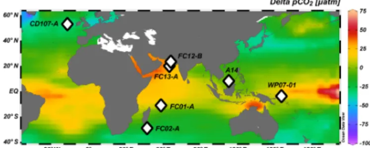
WP07-01 −3.93 156.00 1800 non-upwelling 7300–8600c A14 8.02 113.39 1911 non-upwelling 7300–8600c 806 A 0.32 159.36 2521 equatorial divergence 7300–8600c 807 A 3.61 156.62 2804 equatorial divergence 7300–8600c a_{Thomson et al., 2000.}b_{Wilson et al., 2012.}c_{Age for core top of site 806B from Lea et al. (2000).}

Figure 2. Map showing locations of the core tops used in this study (white diamonds). Red open circles represent the sites used for in situ carbonate parameters from the GLODAP database (Key et al., 2004).

3 Materials and methods 3.1 Localities studied

Core-top locations were selected to span a broad range of seawater pH, carbonate system parameters, and oceanic regimes. Samples from the Atlantic Ocean (CD107-A), In-dian Ocean (FC-01a and FC-02a), Arabian Sea (FC-13a and FC-12b), and Pacific Ocean (WP07-01, A14, and Ocean Drilling Program 806A and 807A) were analyzed; charac-teristics of the sites are summarized in Tables 1 and S7 and Figs. 2 and 3.

Atlantic site CD107-a (CD107 site A) was cored in 1997 by the Benthic Boundary Layer program (BENBO) (Black, 1997 – cruise report RRS Charles Darwin cruise 107). Ara-bian Sea sites FC-12b (CD145 A150) and FC-13a (CD145 A3200) were retrieved by the Charles Darwin in the

Pak-istan margin in 2004 (Bett, 2004 – cruise report no. 50 RRS Charles Darwincruise 145). A14 was recovered by a box corer in the southern area of the South China Sea in 2012. Core WP07-01 was obtained from the Ontong Java Plateau using a giant piston corer during the Warm Pool Subject Cruise in 1993. Holes 806A and 807A were retrieved on Leg 130 by the Ocean Drilling Program (ODP). The top 10 cm of sediment from CD107-A has been radiocarbon dated to be Holocene <3 kyr (Thomson et al., 2000). Samples from multiple box cores from Indian Ocean sites were radiocar-bon dated as Holocene <7.3 kyr (Wilson et al., 2012). Sam-ples from western equatorial Pacific site 806B, close to site WP07-01, are dated to between 7.3 and 8.6 kyr (Lea et al., 2000). Arabian Sea and Pacific core-top samples were not radiocarbon dated but are assumed to be Holocene.

3.2 Species

Around 50–100 foraminifera shells were picked from the 400 to 500 µm fraction size for Globorotalia menardii and Globorotalia tumida, >500 µm for Orbulina universa, and from the 250–400 µm fraction size for Trilobatus sacculifer (w/o sacc, without sacc-like final chamber), Trilobatus sac-culifer(sacc, sacc-like final chamber), Globigerinoides ruber (white, sensu stricto), Neogloboquadrina dutertrei, and Pul-leniatina obliquiloculata. The samples picked for analyses were visually well preserved.

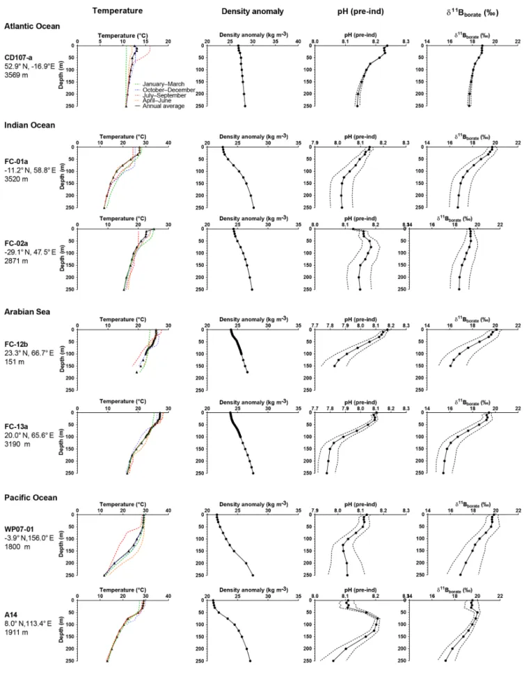
Figure 3. Preindustrial data versus depth for the sites used in this study. The figure shows seasonal temperatures (extracted from World Ocean Database 2013), density anomaly (kg m−3), and preindustrial pH and preindustrial δ11B of H₄BO−₄ (calculated from the GLODAP database and corrected for anthropogenic inputs). Dotted lines are the calculated uncertainties based on errors on TA and DIC from the GLODAP database.

3.3 Sample cleaning

Briefly, picked foraminifera were gently cracked open, clay was removed with successive ultrasonication steps in MQ water and methanol, and then they were checked for coarse-grained silicates. The next stages of sample processing and chemical separation were performed in a class 1000 clean lab equipped with boron-free HEPA filters. Samples were cleaned using full reductive and oxidative cleaning (Boyle, 1981; Boyle and Keigwin, 1985; Barker et al., 2003). Sam-ples from the South China Sea (sites A14, E035) presented high Mn and high Fe. Due to potential Fe-Mn oxide and hy-droxides the reductive cleaning was used. Previous compar-isons of cleaning methods have shown there is no impact of the reductive step on B/Ca (Misra et al., 2014b), but there is an impact of the reductive step on Mg/Ca (Barker et al., 2003 and others). Nevertheless, it is possible that Fe-Mn oxide and hydroxides can result in non-negligible Mg and B contami-nation. Because this study was designed to investigate boron proxies and in order to be consistent in methodology, the re-ductive cleaning was used at all sites. Cleaned samples se-lected for this study did not yield high Mn concentrations (see Supplement for discussion on contamination).

A final leaching step with 0.001 N HCl was done before dissolution in 1 N HCl. Hydrochloric acid was used to allow complete dissolution of the sample including Fe-Mn oxide and hydroxides if present. Each sample was divided into two aliquots: an aliquot for boron purification and one aliquot for trace element analysis.

3.4 Reagents

Double-distilled HNO3and HCl acids (from Merck®grade)

and a commercial bottle of ultrapure-grade HF were used at Brest. Double-distilled acids were used at Cambridge. All acids and further dilutions were prepared using double-distilled 18.2 M cm−1 MQ water. Working standards for isotope ratio and trace element measurements were freshly diluted on a daily basis with the same acids used for sample preparation to avoid any matrix effects.

3.5 Boron isotopes

Boron purification for isotopic measurement was done uti-lizing the microdistillation method developed by Gaillardet et al. (2001) for Ca-rich matrices by Wang et al. (2010) and adapted at Cambridge by Misra et al. (2014a). A total of 70 µL of carbonate sample dissolved in 1 N HCl was loaded on a cap of a clean fin legged 5 mL conical beaker upside down. The tightly closed beaker was put on a hot plate at 95◦C for 15 h. The beakers were taken off the hot plate and were allowed to cool for 15 min. The cap where the residue formed was replaced by a clean one. Then, 100 µL of 0.5 % HF was added to the distillate.

Boron isotopic measurements were carried out on a Thermo Scientific® Neptune+ MC-ICP-MS at the Univer-sity of Cambridge. The Neptune+ was equipped with a Jet interface and two 1013resistors. The instrumental setup in-cluded Savillex® 50 µL min−1 C-flow self-aspirating nebu-lizer, a single-pass Teflon® Scott-type spray chamber con-structed utilizing Savillex® column components, a 2.0 mm Pt injector from ESI®, a Thermo® Ni “normal”-type sam-ple cone, and ‘X’ type skimmer cones. Both isotopes of boron were determined utilizing 1013 resistors (Misra et al., 2014a; Lloyd et al., 2018).

The sample size for boron isotope analyses typically ranged from 10 ppb B (∼ 5 ng B) to 20 ppb B samples (∼ 10 ng B). Instrumental sensitivity for11B was 17 mV ppb−1 B (e.g., 170 mV for 10 ppb B) in wet plasma at a 50 µL min−2 sample aspiration rate. Intensity of 11B for a sample at 10 ppb B was typically 165 mV ± 5 mV, which closely matched the 170 mV ± 5 mV of the standard. Due to the low boron content of the samples, extreme care was taken to avoid boron contamination during sample preparation and re-duce memory effect during analysis. Procedural boron blanks ranged from 15 to 65 pg B and contributed to less than <1 % of the sample signal. The acid blank during analyses was measured at ≤ 1 mV on11B, meaning a contribution <1 % of the sample intensity; no memory effect was observed within and across sessions. No matrix effect resulting from the mix HCl/HF was observed on the δ11B.

Analyses of external standards were done to ensure data quality. For δ11B measurements one carbonate standard and one coral were utilized: the JCp-1 (Geological Survey of Japan, Tsukuba, Japan) international standard (Gutjahr et al., 2014) and the NEP coral (Porites sp., δ11B = 26.12±0.92 ‰, 2SD, n = 33, Holcomb et al., 2015, and Sutton et al., 2018, Table S2 in the Supplement) from University of Western Australia–Australian National University. A certified boric acid standard, the ERM© AE121 (δ11B = 19.9 ± 0.6 ‰, SD, certified), was used to monitor reproducibility and drift dur-ing each session (Vogl and Rosner, 2011; Foster et al., 2013; Misra et al., 2014b). Results for the isotopic composition of the NEP coral are shown in Table S2, average values are δ11BNEP=25.70 ± 0.93 ‰ (2SD, n = 22) over seven

differ-ent analytical sessions with each number represdiffer-enting an ab initio processed sample. Our results are within error of pub-lished values of 26.20 ± 0.88 ‰ (2SD, n = 27) and 25.80 ± 0.89 ‰ (2SD, n = 6) by Holcomb et al. (2015) and Sutton et al. (2018), respectively. Chemically cleaned JCp-1 samples were measured at 24.06 ± 0.20 (2SD, n = 6) and are within error of published values of 24.37±0.32 ‰, 24.11±0.43 ‰, and 24.42 ± 0.28 ‰ by Holcomb et al. (2015), Farmer et al. (2016), and Sutton et al. (2018), respectively.

3.6 Trace elements

The calcium concentration of each sample was measured on an inductively coupled plasma atomic emission

ter (ICP-AES) Ultima 2 HORIBA at the Pôle spectrome-trie Océan (PSO), UMR6538 (Plouzané, France). Samples were then diluted to fixed calcium concentrations (typically 10 ppm or 30 ppm Ca) using 0.1 M HNO3 and 0.3 M HF

matching multielement standard Ca concentration to avoid any matrix effects (Misra et al., 2014b). Levels of remaining HCl (<1 %) in these diluted samples were negligible and did not contribute to matrix effects. Trace elements (e.g., X/Ca ratios) were analyzed on a Thermo Scientific®Element XR high-resolution inductively coupled plasma mass spectrome-ter (HR-ICP-MS) at the PSO, Ifremer (Plouzané, France).

Trace element analyses were done at a Ca concentra-tion of 10 or 30 ppm. The typical blanks for a 30 ppm Ca session were 7Li <2 %, 11B <7 %, 25Mg <0.2 %, and

43_{Ca <0.02 %. Additionally, blanks for a 10 ppm Ca}

ses-sion were 7Li <2.5 %, 11B <10 %, 25Mg <0.4 %, and

43_{Ca <0.05 %. Due to strong memory effect for boron and}

instrumental drift on the Element XR, long sessions of con-ditioning were done prior to analyses. Boron blanks were driven below 5 % of signal intensity usually after 4 to 5 d of continuous analyses of carbonate samples. External re-producibility was determined on the consistency standard Cam-Wuellestorfi (courtesy of the University of Cambridge) (Misra et al., 2014b), Table S3. Our X/Ca ratio measure-ments on the external standard Cam-Wuellestorfi were within error of the published value all the time (Table S3), vali-dating the robustness of our trace element data. Analytical uncertainty of a single measurement was calculated from the reproducibility of the Cam-Wuellestorfi, measured dur-ing a particular mass spectrometry session. The analytical uncertainties (2SD, n = 31, Table S3) on the X/Ca ratios are ±0.4 µmol mol−1for Li/Ca, ±7 µmol mol−1for B/Ca, and ±0.01 µmol mol−1for Mg/Ca, respectively.

3.7 Oxygen isotopes

Carbonate δ13C and δ18O were measured on a GasBench II coupled to a Delta V mass spectrometer at the stable iso-tope facility of Pôle spectrometrie Océan (PSO), Plouzané. Around 20 shells were weighed, crushed, and had clay re-moved following the same method described in Sect. 3.3 (Barker et al., 2003). The recovered foraminifera were weighed in tubes and flushed with He gas. Samples were then digested in phosphoric acid and analyzed. Results were cali-brated to the Vienna Pee Dee Belemnite (VPDB) scale by in-ternational standard NBS19, and analytical precision on the in-house standard Ca21 was better than ±0.11 ‰ for δ18O (SD, n = 5) and ±0.03 ‰ for δ13C (SD, n = 5).

3.8 Calcification depth determination

We utilized two different chemo-stratigraphic methods to es-timate the calcification depth (CD) in this study (Tables S6 and S7). The first method (CD1), commonly used in pale-oceanography, utilizes δ18O measurements of the carbonate

(δ18Oc) to estimate calcification depths (referred to as δ18

O-based calcification depths) (Schmidt et al., 2002; Mortyn et al., 2003; Sime et al., 2005; Farmer et al., 2007; Birch et al., 2013). Rebotim et al. (2017) also showed good cor-respondence between living depth habitat and calcification depth derived using CD1. The second method (CD2) utilizes Mg/Ca-based temperature estimates (TMg/Ca) to constrain

calcification depths (Quintana Krupinski et al., 2017). How-ever, we note that reductive cleaning leads to a decrease in Mg/Ca that in turn would result in a bias towards deeper cal-cification depths, which is not the case when we utilize non-Mg/Ca-based methodologies. In both cases, the prerequisite was that vertical profiles of seawater temperature are avail-able for different seasons in ocean atlases and cruise reports and that hydrographic data and geochemical proxy signatures can be compared to assess the depth in the water column that represents the taxon’s maximum abundance.

Because both methods have their uncertainties (in one case use of taxon-specific calibrations and in the other analyti-cal limitations), both estimates of analyti-calcification depth were compared to published values for the basin (CD3) and where available for the same site (Table S6). To select which calci-fication depth to use for further calculations, we first looked at CD1, CD2, and CD3. If CD1 and CD2 were similar we

se-lected this calcification depth, and if CD1and CD2were

dif-ferent we chose literature values, CD3, when available. For

some less studied species, like G. tumida, G. menardii, or P. obliquiloculata, CD3 was not always available but when

available showed good correspondence with our CD2.

More-over due to availability of Mg/Ca-derived temperature taxon-specific calibrations, we preferentially use CD2 for those

species.

We applied (based on uncertainties of our measurements) an uncertainty of ±10 m for calcification depths >70 m and an uncertainty of ±20 m when calcification depths <70 m. Direct observations of living depths of foraminifera remain limited. However, the depth uncertainties reported here are in line with the uncertainties calculated based on direct ob-servations in the eastern North Atlantic which give a stan-dard error on average living depths ranging from 6 to 22 m for the same species (Rebotim et al., 2017). The decrease in Mg/Ca due to reductive cleaning was not taken into account because it has not been studied for most of the species used in this study and because the depth uncertainty applied based on δ18O analytical error is conservative relative to the uncer-tainty of a 10 % decrease in Mg/Ca equivalent that would be equivalent to ∼ 1.2◦_{C. The depth habitats utilized to derive}

in situ parameters are summarized in Table S7. 3.9 δ11Bborate

Two carbonate system parameters are needed to fully con-strain the carbonate system. Following the approach of Fos-ter et al. (2008), we used the GLODAP database (Key et al., 2004) corrected for anthropogenic inputs in order to

esti-mate preindustrial carbonate system parameters at each site. Temperature, salinity, and pressure for each site are from the World Ocean Database 2013 (Boyer et al., 2013). We utilized the R© code in Henehan et al. (2016) (courtesy of Michael Henehan) to calculate the δ11Bborate and δ11Bborate

uncer-tainty and derive our calibrations. Unceruncer-tainty for δ11Bborate

utilizing Henehan’s code was similar to uncertainty calcu-lated by applying 2SD of the δ11Bborate profiles within the

limits imposed by our calcification depth.

The MATLAB© template provided by Zeebe and Wolf-Gladow (2001) was used to calculate pCO2from TA;

tem-perature, salinity, and pressure were included in the calcu-lations. Total boron was calculated from Lee et al. (2010), and K1and K2were calculated from Mehrbach et al. (1973)

refitted by Dickson and Millero (1987).

Statistical tests were performed utilizing GraphPad© soft-ware, and linear regressions for calibration were derived uti-lizing R© code in Henehan et al. (2016) (courtesy of Michael Henehan) with k (number of wild bootstrap replicates) equal to 500.

4 Results

4.1 Depth habitat

The calcification depths utilized in this paper are summarized in Tables S6 and S7, including a comparison of tion depth determination methods. The calculated calcifica-tion depths are consistent with the ecology of each species and the physical properties of the water column of the sites. Specimens of G. ruber and T. sacculifer appear to be living in the shallow mixed layer (0–100 m), with T. sacculifer living or migrating deeper than G. ruber (down to 125 m). Speci-mens of O. universa and P. obliquiloculata are living in the upper thermocline; G. menardii is found in the upper ther-mocline until the therther-mocline depth specific to the location; N. dutertreiis living near thermocline depths and G. tumida is found in the lower thermocline.

Data from the multiple approaches for calculating calcifi-cation depth (CD1, CD2, and CD3) imply that some species inhabit deeper environments in the western equatorial Pacific (WEP) relative to the Arabian Sea, which in turn are deeper-dwelling than the same morphospecies occurring in the In-dian Ocean. In some cases, we find evidence for differences in habitat depth of up to ∼ 100 m between the WEP and the Arabian Sea. This trend is observed for G. ruber and T. sac-culifer, but not for O. universa.

Some differences are observed between the two methods for calcification depth determination that are based on δ18O and Mg/Ca (CD1 and CD2). These differences might be due to the choice of calibration. Alternatively, our uncertainties for δ18O imply larger uncertainties on calcification depth de-terminations that use this approach, compared to Mg/Ca-based estimates.

4.2 Empirical calibrations of foraminiferal δ11Bcarbonateto δ11Bborate

Results for the different species analyzed in this study are presented in Figs. 4 and 5 and summarized in Table 2; ad-ditionally, published calibrations for comparison are summa-rized in Table 3.

4.2.1 G. ruber

Samples were picked from the 250–300 µm fraction, except for the WEP sites where G. ruber shells were picked from the 250–400 µm fraction. Weight per shell averaged 11±4 µg (n = 4, SD), although the weight was not measured on the same subsample analyzed for δ11B and trace elements or at the WEP sites. In comparison to literature, the size fraction used for this study was smaller: Foster et al. (2008) used the 300–355 µm fraction, Henehan et al. (2013) utilized mul-tiple size fractions (250–300, 250–355, 300–355, 355–400, and 400–455 µm), and Raitzsch et al. (2018) used the 315– 355 µm fraction.

Our results for G. ruber (Fig. 4) are in close agreement with published data from other core tops, sediment traps, tows, and culture experiments for δ11Bborate>19 ‰ (Foster

et al., 2008; Henehan et al., 2013; Raitzsch et al., 2018). However, the two data points from δ11Bborate<19 ‰ are

lower compared to previous studies. Elevated δ11Bcarbonate

values relative to δ11Bborate have been explained by the high

photosynthetic activity of symbionts (Hönisch et al., 2003; Zeebe et al., 2003). Three calibrations have been derived (Ta-ble 3). Linear regression on our data alone yields a slope of 1.12 (±1.67). The uncertainty is significant given limited data in our study, and given this large uncertainty, our sen-sitivity of δ11Bcarbonate to δ11Bborate is also consistent with

the low sensitivity trend of culture experiments from Sanyal et al. (2001) or Henehan et al. (2013). The second calibra-tion made compiling all data from literature shows a sensi-tivity similar (e.g., 0.46 (±0.34)) to the one recently pub-lished by Raitzsch et al. (2018) (e.g., 0.45 (±0.16), Table 3). The third linear regression made only on data from the 250– 400 µm fraction from our study and from the 250–300 µm fraction from Henehan et al. (2013) yields a sensitivity of 0.58 (±0.91) similar to culture experiments from Henehan et al. (2013) (e.g., 0.6 (±0.16), Table 3). This third calibration is offset by ∼ −0.4 ‰ (p>0.05) compared to culture cali-bration from Henehan et al. (2013).

4.2.2 T. sacculifer

δ11Bcarbonateresults for T. sacculifer (sacc and without sacc)

(Fig. 4) are compared to published data (Foster et al., 2008; Martínez-Boti et al., 2015b; Raitzsch et al., 2018). Results for T. sacculiferare in good agreement with the literature and ex-hibit higher δ11Bcarbonatecompared to expected δ11Bborateat

T able 2. Analytical results of δ 13 C, δ 18 O, and δ 11 B and elemental ratios Li / Ca, B / Ca, and Mg / Ca. Core Species Fraction size (µm) δ₁₃ C a δ₁₈ O a δ₁₁ Bc 1 δ₁₁ Bc 2 δ₁₁ B b av erage Li / Ca c B / Ca c Mg / Ca c Mn / Ca c Fe / Ca c (‰) (‰) (‰) (‰) (‰) (µmol mol − 1 ) (µmol mol − 1 ) (mmol mol − 1 ) (µmol mol − 1 ) (mmol mol − 1 ) Atlantic Ocean CD107a O. univer sa > 500 1.99 ± 0.03 1.25 ± 0.11 16.85 ± 0.31 (2SD, nAE121 = 11) 16.95 ± 0.31 (2SD, nAE121 = 11) 16.90 ± 0.22 13.9 ± 0.4 68 ± 7 3.60 ± 0.01 13 ± 7 0.16 ± 0.01 Indian Ocean FC-01a G. ruber (white ss) 250–300 1.37 ± 0.03 − 1.32 ± 0.11 19.33 ± 0.31 (2SD, nAE121 = 11) 19.41 ± 0.31 (2SD, nAE121 = 11) 19.37 ± 0.22 15.4 ± 0.4 109 ± 7 3.98 ± 0.01 10 ± 7 0.07 ± 0.01 FC-01a T . sacculifer (sacc) 300–400 1.88 ± 0.03 − 2.20 ± 0.11 18.71 ± 0.24 (2SD, nAE121 = 10) 18.73 ± 0.24 (2SD, nAE121 = 10) 18.72 ± 0.17 12.1 ± 0.4 87 ± 7 3.45 ± 0.01 9 ± 7 0.03 ± 0.01 FC-01a T . sacculifer (without sacc) 300–400 2.02 ± 0.03 − 1.05 ± 0.11 19.13 ± 0.24 (2SD, nAE121 = 10) 19.32 ± 0.24 (2SD, nAE121 = 10) 19.23 ± 0.17 12.1 ± 0.4 82 ± 7 3.42 ± 0.01 14 ± 7 0.03 ± 0.01 FC-01a O. univer sa > 500 15.50 ± 0.26 ( 2SD, nAE121 = 14) 15.50 ± 0.26 FC-01a P . obliquiloculata 300–400 1 .00 ± 0 .03 − 0.55 ± 0.11 16.40 ± 0.26 (2SD, nAE121 = 14) 16.10 ± 0.26 (2SD, nAE121 = 14) 16.25 ± 0.18 15.4 ± 0.4 78 ± 7 2.06 ± 0.01 14 ± 7 0.05 ± 0.01 FC-01a G. menar dii 300–400 1.64 ± 0.03 0.43 ± 0.11 17.52 ± 0.26 (2SD, nAE121 = 14) 17.69 ± 0.26 (2SD, nAE121 = 14) 17.60 ± 0.18 12.7 ± 0.4 63 ± 7 2.26 ± 0.01 8 ± 7 0.07 ± 0.01 FC-01a N. dutertr ei 300–400 1.28 ± 0.03 − 0.43 ± 0.11 16.40 ± 0.31 (2SD, nAE121 = 11) 16.59 ± 0.31 (2SD, nAE121 = 11) 16.50 ± 0.22 18.6 ± 0.4 73 ± 7 1.81 ± 0.01 11 ± 7 0.03 ± 0.01 FC-01a G. tumida 300–400 1.29 ± 0.03 − 0.53 ± 0.11 16.21 ± 0.31 (2SD, nAE121 = 11) 16.18 ± 0.31 (2SD, nAE121 = 11) 16.20 ± 0.22 10.0 ± 0.4 61 ± 7 1.79 ± 0.01 11 ± 7 0.02 ± 0.01 FC-02a G. ruber (white ss) 250–300 0.30 ± 0.03 − 1.40 ± 0.11 20.02 ± 0.24 (2SD, nAE121 = 10) 19.90 ± 0.24 (2SD, nAE121 = 10) 19.96 ± 0.17 18.2 ± 0.4 125 ± 7 3.47 ± 0.01 10 ± 7 0.07 ± 0.01 FC-02a T . sacculifer (sacc) 300–400 1.43 ± 0.03 − 1.60 ± 0.11 20.07 ± 0.24 (2SD, nAE121 = 10) 19.93 ± 0.24 (2SD, nAE121 = 10) 20.00 ± 0.17 14.2 ± 0.4 106 ± 7 3.30 ± 0.01 10 ± 7 0.03 ± 0.01 FC-02a O. univer sa > 500 1.79 ± 0.03 0.02 ± 0.11 18.05 ± 0.26 (2SD, nAE121 = 14) 17.97 ± 0.26 (2SD, nAE121 = 14) 18.01 ± 0.18 14.8 ± 0.4 67 ± 7 4.40 ± 0.01 11 ± 7 0.05 ± 0.01 FC-02a P . obliquiloculata 300–400 0.34 ± 0.03 0.56 ± 0.11 16.35 ± 0.26 (2SD, nAE121 = 14) 16.69 ± 0.26 (2SD, nAE121 = 14) 16.52 ± 0.18 16.6 ± 0.4 83 ± 7 2.33 ± 0.01 7 ± 7 0.03 ± 0.01 FC-02a G. menar dii 300–400 1.73 ± 0.03 − 0.51 ± 0.11 17.77 ± 0.26 (2SD, nAE121 = 14) 17.77 ± 0.26 15.8 ± 0.4 125 ± 7 2.21 ± 0.01 17 ± 7 0.03 ± 0.01 FC-02a N. dutertr ei 300–400 1.03 ± 0.03 − 0.55 ± 0.11 16.78 ± 0.31 (2SD, nAE121 = 11) 17.03 ± 0.31 (2SD, nAE121 = 11) 16.91 ± 0.22 18.6 ± 0.4 82 ± 7 2.13 ± 0.01 13 ± 7 0.07 ± 0.01 FC-02a G. tumida 300–400 1.64 ± 0.03 − 0.28 ± 0.11 16.93 ± 0.26 (2SD, nAE121 = 14) 16.95 ± 0.26 (2SD, nAE121 = 14) 16.94 ± 0.18 15.6 ± 0.4 87 ± 7 1.90 ± 0.01 17 ± 7 0.04 ± 0.01 Arabian Sea FC-12b G. ruber (white ss) 250–300 0.58 ± 0.03 − 2.82 ± 0.11 21.30 ± 0.31 (2SD, nAE121 = 11) 21.23 ± 0.31 (2SD, nAE121 = 11) 21.26 ± 0.22 19.5 ± 0.4 164 ± 7 5.76 ± 0.01 14 ± 7 0.16 ± 0.01 FC-12b T . sacculifer (sacc) 300–400 1.76 ± 0.03 − 2.15 ± 0.11 19.65 ± 0.31 (2SD, nAE121 = 11) 19.57 ± 0.31 (2SD, nAE121 = 11) 19.61 ± 0.22 14.6 ± 0.4 101 ± 7 4.28 ± 0.01 17 ± 7 0.14 ± 0.01 FC-12b T . sacculifer (without sacc) 300–400 1.97 ± 0.03 − 2.19 ± 0.11 20.32 ± 0.31 (2SD, nAE121 = 11) 20.37 ± 0.31 (2SD, nAE121 = 11) 20.34 ± 0.22 16.7 ± 0.4 116 ± 7 4.90 ± 0.01 20 ± 7 0.26 ± 0.01 FC-12b O. univer sa > 500 1.89 ± 0.03 − 1.59 ± 0.11 18.13 ± 0.20 (2SD, nAE121 = 6) 18.13 ± 0.20 13.6 ± 0.4 103 ± 7 6.91 ± 0.01 10 ± 7 0.06 ± 0.01 FC-12b P . obliquiloculata 300–400 0.5 ± 0.03 − 1.58 ± 0.11 16.45 ± 0.26 (2SD, nAE121 = 14) 16.15 ± 0.26 (2SD, nAE121 = 14) 16.30 ± 0.18 16.7 ± 0.4 95 ± 7 3.61 ± 0.01 69 ± 7 0.38 ± 0.01 FC-12b G. menar dii 300–400 1.05 ± 0.03 − 0.97 ± 0.11 16.2 ± 0.26 (2SD, nAE121 = 14) 16.20 ± 0.26 14.8 ± 0.4 75 ± 7 3.44 ± 0.01 52 ± 7 0.17 ± 0.01 FC-12b N. dutertr ei 300–400 1.35 ± 0.03 − 1.57 ± 0.11 17.77 ± 0.24 (2SD, nAE121 = 10) 17.73 ± 0.24 (2SD, nAE121 = 10) 17.75 ± 0.17 17.1 ± 0.4 75 ± 7 3.25 ± 0.01 46 ± 7 0.25 ± 0.01 FC-13a G. ruber (white ss) 250–300 0.08 ± 0.03 − 3.71 ± 0.11 20.27 ± 0.24 (2SD, nAE121 = 10) 20.15 ± 0.24 (2SD, nAE121 = 10) 20.21 ± 0.17 16.4 ± 0.4 147 ± 7 4.52 ± 0.01 13 ± 7 0.08 ± 0.01 FC-13a T . sacculifer (without sacc) 300–400 1.59 ± 0.03 − 2.46 ± 0.11 17.85 ± 0.29 (2SD, nAE121 = 12) 17.85 ± 0.29 15.7 ± 0.4 121 ± 7 5.49 ± 0.01 21 ± 7 0.49 ± 0.01 FC-13a P . obliquiloculata 300–400 0.00 ± 0.03 − 0.97 ± 0.11 16.51 ± 0.26 (2SD, nAE121 = 14) 16.50 ± 0.26 (2SD, nAE121 = 14) 16.51 ± 0.18 18.7 ± 0.4 79 ± 7 4.43 ± 0.01 30 ± 7 0.43 ± 0.01 FC-13a G. menar dii 300–400 0.75 ± 0.03 − 1.07 ± 0.11 16.74 ± 0.20 (2SD, nAE121 = 6) 16.74 ± 0.20 9.2 ± 0.4 60 ± 7 1.99 ± 0.01 19 ± 7 0.07 ± 0.01 FC-13a N. dutertr ei 300–400 0.71 ± 0.03 − 1.41 ± 0.11 14.43 ± 0.24 (2SD, nAE121 = 10) 14.40 ± 0.24 (2SD, nAE121 = 10) 14.41 ± 0.17 15.7 ± 0.4 69 ± 7 1.98 ± 0.01 15 ± 7 0.06 ± 0.01 P acific Ocean WP07-a G. ruber (white ss) 250–400 19.12 ± 0.29 (2SD, nAE121 = 12) 19.12 ± 0.29 14.5 ± 0.4 144 ± 7 4.32 ± 0.01 15 ± 7 0.16 ± 0.01 WP07-a T . sacculifer (sacc) 250–400 20.13 ± 0.21 (2SD, nAE121 = 11) 20.13 ± 0.21 12.7 ± 0.4 92 ± 7 4.44 ± 0.01 22 ± 7 0.05 ± 0.01 WP07-a T . sacculifer (without sacc) 250–400 18.10 ± 0.31 (2SD, nAE121 = 11) 18.04 ± 0.31 (2SD, nAE121 = 11) 18.07 ± 0.22 12.3 ± 0.4 192 ± 7 4.51 ± 0.01 21 ± 7 0.08 ± 0.01 WP07-a O.univer sa 500–630 18.13 ± 0.26 (2SD, nAE121 = 14) 17.99 ± 0.26 (2SD, nAE121 = 14) 18.06 ± 0.18 11.9 ± 0.4 71 ± 7 7.52 ± 0.01 11 ± 7 0.02 ± 0.01 WP07-a P . obliquiloculata 250–400 16.08 ± 0.26 (2SD, nAE121 = 14) 16.19 ± 0.26 (2SD, nAE121 = 14) 16.14 ± 0.18 13.4 ± 0.4 72 ± 7 3.02 ± 0.01 7 ± 7 0.03 ± 0.01 WP07-a G. menar dii 250–400 14.74 ± 0.26 (2SD, nAE121 = 14) 14.53 ± 0.26 (2SD, nAE121 = 14) 14.64 ± 0.18 13.5 ± 0.4 85 ± 7 2.68 ± 0.01 26 ± 7 0.08 ± 0.01 WP07-a N. dutertr ei 250–400 16.91 ± 0.31 (2SD, nAE121 = 11) 16.99 ± 0.31 (2SD, nAE121 = 11) 16.95 ± 0.22 21.7 ± 0.4 86 ± 7 3.66 ± 0.01 42 ± 7 0.63 ± 0.01 WP07-a G. tumida 250–400 16.45 ± 0.26 (2SD, nAE121 = 14) 16.32 ± 0.26 (2SD, nAE121 = 14) 16.39 ± 0.18 10.6 ± 0.4 58 ± 7 2.55 ± 0.01 16 ± 7 0.10 ± 0.01 806A T . sacculifer (without sacc) 250–400 17.53 ± 0.36 (2SD, nAE121 = 11) 17.53 ± 0.36 14.40 ± 0.4 77 ± 7 3.89 ± 0.01 7 ± 7 0.15 ± 0.01 807A T . sacculifer (without sacc) 250–400 18.38 ± 0.21 (2SD, nAE121 = 11) 18.17 ± 0.21 (2SD, nAE121 = 11) 18.28 ± 0.15 12.54 ± 0.4 87 ± 7 4.24 ± 0.01 17 ± 7 0.09 ± 0.01 A14 G. ruber (white ss) 250–400 18.91 ± 0.24 (2SD, nAE121 = 10) 19.17 ± 0.24 (2SD, nAE121 = 10) 19.04 ± 0.17 A14 T . sacculifer (sacc) 250–400 19.53 ± 0.24 (2SD, nAE121 = 10) 19.32 ± 0.24 (2SD, nAE121 = 10) 19.42 ± 0.17 12.0 ± 0.4 102 ± 7 3.91 ± 0.01 22 ± 7 0.02 ± 0.01 A14 T . sacculifer (without sacc) 250–400 18.93 ± 0.24 (2SD, nAE121 = 10) 18.84 ± 0.24 (2SD, nAE121 = 10) 18.88 ± 0.17 12.3 ± 0.4 93 ± 7 3.76 ± 0.01 25 ± 7 0.06 ± 0.01 A14 O. univer sa 500–560 17.33 ± 0.26 (2SD, nAE121 = 14) 17.08 ± 0.26 (2SD, nAE121 = 14) 17.20 ± 0.18 11.3 ± 0.4 66 ± 7 6.59 ± 0.01 10 ± 7 0.02 ± 0.01 A14 N. dutertr ei 250–400 14.39 ± 0.31 (2SD, nAE121 = 11) 14.39 ± 0.31 16.9 ± 0.4 75 ± 7 1.99 ± 0.01 35 ± 7 0.04 ± 0.01 a Uncertainties gi v en in 1SD (see te xt). b When tw o measurements were carried out uncertainty w as calculated with 1a = q (1 / P i (₁ /1 a i )2 ) ; with only one measurement the error w as determined on reproducibility of the AE121 standard. c Uncertainty gi v en in 2SD, calculated on the reproducibility of Cam-W uellestorfi (see te xt and T able S3, reference in Misra et al., 2014a).

T able 3. Species-specific δ 11 Bcarbonate -to-δ 11 Bborate calibrations from literature and from our data. Species Size fraction Material Instrument Re gression δ 11 Bborate = f (δ 11 Bcalcite ) n Calibration Reference (µm) (original) method number G. ruber ∼ 380 Culture/core tops/plankton to ws MC-ICP-MS δ 11 Bborate = [δ 11 Bcalcite − 9 .52 ( ± 2 .02 ) ]/ 0 .6 ( ± 0 .11 ) Henehan et al. (2013) G. ruber 315–355 Core tops MC-ICP-MS δ 11 Bborate = [δ 11 Bcalcite − 11 .78 ( ± 3 .20 ) ]/ 0 .45 ( ± 0 .16 ) Raitzsch et al. (2018) T . sacculifer n.d. Culture/artificial sea w ater enriched in B N-TIMS δ 11 Bborate = [δ 11 Bcalcite − 3 .94 ( ± 4 .02 ) ]/ 0 .82 ( ± 0 .22 ) San yal et al. (2001) refitted Martínez-Boti et al. (2015) T . sacculifer 315–355 Core tops MC-ICP-MS δ 11 Bborate = [δ 11 Bcalcite − 8 .86 ( ± 5 .27 ) ]/ 0 .59 ( ± 0 .21 ) Raitzsch et al. (2018) O. univer sa no ef fect Core tops/plankton to ws/sediment traps MC-ICP-MS δ 11 Bborate = [δ 11 Bcalcite + 0 .42 ( ± 2 .85 ) ]/ 0 .95 ( ± 0 .17 ) Henehan et al. (2016) O. univer sa > 425 Core tops MC-ICP-MS δ 11 Bborate = [δ 11 Bcalcite + 5 .69 ( ± 7 .51 ) ]/ 1 .26 ( ± 0 .39 ) Raitzsch et al. (2018) G. b ulloides 300–355 Core top/sediment trap MC-ICP-MS δ 11 Bborate = [δ 11 Bcalcite + 3 .440 ( ± 4 .584 ) ]/ 1 .074 ( ± 0 .252 ) Martínez-Boti et al. (2015) G. b ulloides 315–355 Core tops MC-ICP-MS δ 11 Bborate = [δ 11 Bcalcite + 3 .81 ( ± 13 .17 ) ]/ 1 .13 ( ± 0 .72 ) Raitzsch et al. (2018) N. pac hyderma 150-200 Core tops MC-ICP-MS δ 11 Bborate = δ 11 Bcalcite + 3 .38 Y u et al. (2013) G. ruber 250–400 Core tops MC-ICP-MS Bootstrap δ 11 Bborate = [δ 11 Bcalcite − 9 .11 ( ± 0 .73 ) ]/ 0 .58 ( ± 0 .91 ) 9 0 This study , Henehan et al. (2013) G. ruber 250–400 Core tops MC-ICP-MS Bootstrap δ 11 Bborate = [δ 11 Bcalcite + 1 .23 ( ± 0 .59 ) ]/ 1 .12 ( ± 1 .67 ) 5 1 This study G. ruber 250–455 Core tops MC-ICP-MS Bootstrap δ 11 Bborate = [δ 11 Bcalcite − 11 .73 ( ± 0 .83 ) ]/ 0 .46 ( ± 0 .34 ) 40 2 This study; F oster et al. (2008), Henehan et al. (2016), Raitzsch et al. (2018) T . sacculifer (sacc and without sacc) 250–400 Core tops MC-ICP-MS Bootstrap δ 11 Bborate = [δ 11 Bcalcite + 6 .06 ( ± 0 .25 ) ]/ 1 .38 ( ± 1 .33 ) 11 3 This study T . sacculifer (sacc and without sacc) 250–400 Core tops MC-ICP-MS Bootstrap δ 11 Bborate = [δ 11 Bcalcite − 4 .09 ( ± 0 .86 ) ]/ 0 .83 ( ± 0 .48 ) 27 4 This study; F oster et al. (2008), Raitzsch et al. (2018) N. dutertr ei 300–400 Core tops MC-ICP-MS Bootstrap δ 11 Bborate = [δ 11 Bcalcite − 0 .34 ( ± 1 .83 ) ]/ 0 .93 ( ± 0 .55 ) 5 5 This study N. dutertr ei 300–400 Core tops MC-ICP-MS Bootstrap δ 11 Bborate = [δ 11 Bcalcite − 3 .88 ( ± 0 .65 ) ]/ 0 .72 ( ± 0 .74 ) 9 6 This study; F oster et al. (2008) O. univer sa 400–600 Core tops MC-ICP-MS Bootstrap δ 11 Bborate = [δ 11 Bcalcite + 8 .01 ( ± 23 ) ]/ 1 .38 ( ± 2 .67 ) 5 7 This study O. univer sa 400–600 Core tops MC-ICP-MS Bootstrap δ 11 Bborate = [δ 11 Bcalcite + 2 .08 ( ± 0 .59 ) ]/ 1 .06 ( ± 0 .13 ) 36 8 This study; Henehan et al. (2016), Raitzsch et al. (2018) G. menar dii 400–600 Core tops MC-ICP-MS Bootstrap δ 11 Bborate = [δ 11 Bcalcite − 5 .36 ( ± 1 .36 ) ]/ 0 .65 ( ± 0 .76 ) 5 9 This study G. tumida 400–600 Core tops MC-ICP-MS Bootstrap δ 11 Bborate = [δ 11 Bcalcite − 6 .33 ( ± 2 .52 ) ]/ 0 .57 ( ± 1 .2 ) 3 10 This study P . obliquiloculata 300–400 Core tops MC-ICP-MS Bootstrap δ 11 Bborate = [δ 11 Bcalcite − 5 .59 ( ± 4 .16 ) ]/ 0 .59 ( ± 0 .65 ) 6 11 This study; Henehan et al. (2016) Deep-dweller 300–600 Core tops MC-ICP-MS Bootstrap δ 11 Bborate = [δ 11 Bcalcite − 1 .99 ( ± 0 .13 ) ]/ 0 .82 ( ± 0 .27 ) 22 12 This study Deep-dweller 300–600 Core tops MC-ICP-MS Bootstrap δ 11 Bborate = [δ 11 Bcalcite − 0 .18 ( ± 0 .6 ) ]/ 0 .95 ( ± 0 .13 ) 54 13 This study; F oster et al. (2008), Henehan et al. (2016), Raitzsch et al. (2018) n.d.: not determined.

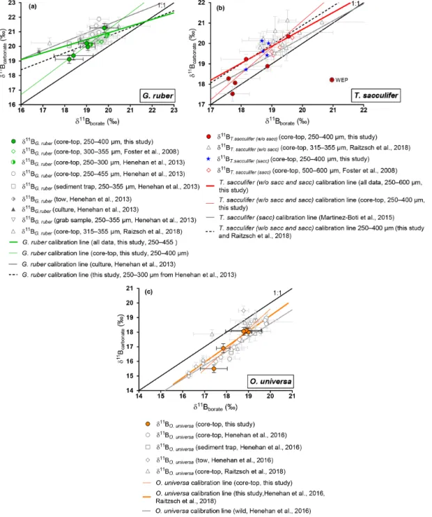
Figure 4. Boron isotopic measurements of mixed-layer foraminifera plotted against δ11Bborate. δ11Bboratewas characterized by

determina-tion of the calcificadetermina-tion depth of foraminifera utilizing data presented in Fig. 3. (a) G. ruber, (b) T. sacculifer, (c) O. universa. Monospecific calibrations (Table 3) and error bars on δ11Bboratewere derived utilizing the wild bootstrap code from Henehan et al. (2016), while errors

on the δ11Bcarbonatefor this study are reported as 2σ of measured AE121 standards during the session of the sample. Calibrations were also

derived on the 250–400 size fraction for G. ruber and T. sacculifer (black dashed lines). Data reported on those graphs have been measured with an MC-ICP-MS.

alone yields a slope of 1.3 ± 0.2 but is not statistically differ-ent to the results from Martínez-Boti et al. (2015b) (Table 3), (p>0.05). However, when compiled with published data us-ing the bootstrap method a slope of 0.83 ± 0.48 is calculated, with a large uncertainty given the variability in the data. It is also noticeable that T. sacculifer (without sacc) samples from

the WEP have a δ11Bcarbonate close to expected δ11Bborate

and are significantly lower compared to the combined T. sac-culiferof other sites (p = 0.01, unpaired t test). When re-gressing data from the 250–400 µm fraction, our results are not significantly different from the regression through data that combine all size fractions (Fig. 4).

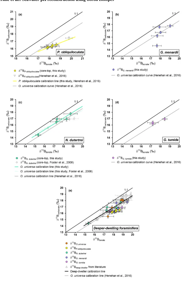
Figure 5. Boron isotopic measurements of deep-dwelling foraminifera (δ11Bcarbonate)plotted against δ11Bborate. δ11Bboratewas constrained

using foraminiferal calcification depths. (a) P. obliquiloculata, (b) G. menardii, (c) N. dutertrei, (d) G. tumida. (e) Compilation of deep dweller species. Monospecific calibrations are summarized in Table 3.

4.2.3 O. universa and deeper-dwelling species: N. dutertrei, P. obliquiloculata, G. menardii , and G. tumida

Our results for O. universa (Fig. 4), N. dutertrei, P. obliquiloculata, G. menardii, and G. tumida (Fig. 5) exhibit lower δ11Bcarbonate compared to the expected δ11Bborate at

their collection location. These data for O. universa are not statistically different from the Henehan et al. (2016) calibra-tion (p>0.05). Our results for N. dutertrei expand upon the initial measurements presented in Foster et al. (2008). The different environments experienced by N. dutertrei in our study permit us to extend the range and derive a calibration for this species; the slope is close to unity (0.93 ± 0.55) and is not significantly different (p>0.05) from the O. universa calibration previously reported by Henehan et al. (2016) (e.g., 0.95 ± 0.17). The data for P. obliquiloculata exhibit the largest offset from the theoretical line. The range of δ11Bborate from the samples we have of G. menardii and

G. tumida is not sufficient to derive calibrations, but the δ11Bcarbonatemeasured for those species is in good agreement

with the N. dutertrei calibration and Henehan et al. (2016) calibration for O. universa.

For O. universa and all deep-dwelling species, the slopes are not statistically different from Henehan et al. (2016) (p>0.05) and are close to unity. If data for deep-dwelling foraminiferal species are pooled together with each other and with data from Henehan et al. (2016) and Raitzch et al. (2018), we calculate a slope of 0.95 (±0.13) (R2= 0.7987, p<0.0001); if only our data are used, we calculate a slope that is not significantly different (0.82±0.27; p<0.05). 4.2.4 Comparison of core-top and culture data

The data for G. ruber and T. sacculifer from the core tops we measured are broadly consistent with previous published results. The calibrations between these core-top-derived es-timates and culture experiments are not statistically differ-ent due to small datasets and uncertainties on the linear re-gressions (Henehan et al., 2013; Marinez-Boti et al., 2015; Raitzsch et al., 2018; Table 3). The sensitivities of the species analyzed are not statistically different and are close to unity. 4.3 B/Ca ratios

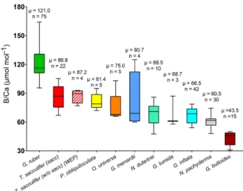
B/Ca ratios are presented in Table 2 and Fig. 6. B/Ca data are species-specific and consistent with previous work (e.g., compiled in Henehan et al., 2016) with ra-tios higher for G. ruber > T. sacculifer (sacc) > T. sac-culifer(without sacc) >P. obliquiloculata > O. universa > >G. menardii> N. dutertrei > G. tumida >G. inflata > N. pachy-derma> G. bulloides (Fig. 6). This study supports species-specific B/Ca ratios as previously published (Yu et al., 2007; Tripati et al., 2009, 2011; Allen and Hönisch, 2012; Henehan et al., 2016). Differences between surface- and

Figure 6. Box plots of B/Ca ratios for multiple foraminifera species., including T. sacculifer (this study; Foster et al., 2008; Ni et al; 2007; Seki et al., 2010), G. ruber (this study; Babila et al., 2014; Foster et al., 2008; Ni et al., 2007), G. inflata, G. bulloides (Yu et al., 2007), N. pachyderma (Hendry et al., 2009; Yu et al., 2013), N. dutertrei (this study; Foster et al., 2008), O. universa, P.obliquiloculata, G. menardii, and G. tumida (this study).

deep-dwelling foraminifera are observed, with lower val-ues and a smaller range for the deeper-dwelling taxa (58–126 µmol mol−1 vs. 83–190 µmol mol−1 for shallow dwellers); however, the trend for the surface dwellers can also be driven by interspecies B/Ca variability. The B/Ca data for deep-dwelling taxa exhibit a significant correlation with [B(OH)−₄]/[HCO−₃](p<0.05) but no correlation with δ11Bcarbonate, and temperature (Fig. S3). Surface-dwelling

species have B/Ca ratios that exhibit significant correlations with [B(OH)−₄]/[HCO−₃], δ11Bcarbonateand temperature. The

sensitivity of B/Ca to [B(OH)−₄]/[HCO−₃] is lower for deep-dwelling species compared to surface-dwelling species. When all the B/Ca data are compiled, significant trends are observed with [B(OH)−₄]/[HCO−₃], δ11Bcarbonate, and

tem-perature (Fig. S3). When comparing data from all sites to-gether, a weak decrease in B/Ca with increasing calcification depth is observed (R2=0.11, p<0.05, Fig. S4). A correla-tion also exists between B/Ca and the water depths of the cores (not significant, Fig. S4).

5 Discussion

5.1 Sources of uncertainty relating to depth habitat and seasonality at studied sites

5.1.1 Depth habitats and δ11Bborate

Because foraminifera will record ambient environmental conditions during calcification, the accurate characterization of in situ data is needed not only for calibrations but also

to understand the reconstructed record of pH or pCO2. The

species we examined are ordered here from shallower to deeper depth habitats: G. ruber > T. sacculifer (sacc) > T. sac-culifer(without sacc) > O. universa > P. obliquiloculata > G. menardii> N. dutertrei > G. tumida (this study; Birch et al., 2013; Farmer et al., 2007), although the specific water depth will vary depending on the physical properties of the water column of the site (Kemle-von Mücke and Oberhänsli, 1999). We note that calculation of absolute calcification depths can be challenging in some cases as many species often transi-tion to deeper waters at the end of their life cycle prior to gametogenesis (Steinhardt et al., 2015).

We find that assumptions about the specific depth habitat a species of foraminifera is calcifying over, in a given region, can lead to differences of a few per mill in calculated iso-topic compositions of borate (Fig. 3). Hence this can cause a bias in calibrations if calcification depths are assumed instead of being calculated (i.e., with δ18O and/or Mg/Ca). Factors including variations in thermocline depth can impact depth habitats for some taxa. At the sites we examined, most of the sampled species live in deeper depth habitats in the WEP rel-ative to the Indian Ocean, which in turn is characterized by deeper depth habitats than in the Arabian Sea. In the tropi-cal Pacific, T. sacculifer is usually found deeper than G. ru-ber except at sites characterized by a shallow thermocline, in which case both species tend to overlap their habitat (e.g., ODP Site 806 in the WEP which has a deeper thermocline than at ODP Site 847 in the eastern equatorial Pacific, EEP) (Rickaby et al., 2005). The difference in depth habitats for T. sacculiferand N. dutertrei between the WEP and EEP can be as much as almost 100 m (Rickaby et al., 2005).

5.1.2 Seasonality and in situ δ11Bborate

As discussed by Raitzsch et al. (2018), depending on the study area, foraminiferal fluxes can change throughout the year. Hydrographic parameters related to carbonate chem-istry may change across seasons at a given water depth. We therefore recalculated the theoretical δ11Bborate using

sea-sonal data for temperature and salinity and annual values for TA and DIC for each depth at each site. The GLODAP (2013) (Key et al., 2004) database does not provide seasonal TA or DIC values.

The low sensitivity of δ11Bborateto temperature and

salin-ity means that calculated δ11Bborate values for each

wa-ter depth at our sites were not strongly impacted (Fig. S1 in the Supplement). Thus, these findings support Raitzsch et al. (2018), who concluded that calculated δ11Bborate

values corrected for seasonality were within the error of non-corrected values for each water depth. As Raitzsch et al. (2018) highlight, seasonality might be more important at high-latitude sites where seasonality is more marked; how-ever, the seasonality of primary production will also be more tightly constrained due to the seasonal progression of

win-ter light limitation and intense vertical mixing and summer nutrient limitation.

Data for our sites suggest that most δ11Bborate variability

we observe does not come from seasonality but from the as-sumed water depths for calcification. With the exception of a few specific areas such as the Red Sea (Henehan et al., 2016; Raitzsch et al., 2018), at most sites examined sea-sonal δ11Bborateat a fixed depth does not vary by more than

∼0.2 ‰. We conclude that seasonality has a relatively mi-nor impact on the carbonate system parameters at the sites we examined.

5.2 δ11B, microenvironment pH, and depth habitats It is common for planktonic foraminifera to have symbi-otic relationships with algae (Gast and Caron, 2001; Shaked and de Vargas, 2006). The family Globigerinidae, includ-ing G. ruber, T. sacculifer, and O. universa, commonly has dinoflagellate algal symbionts (Anderson and Be, 1976; Spero, 1987). The families Pulleniatinidae and Globoro-taliidae (e.g., P. obliquiloculata, G. menardii, and G. tu-mida) have chrysophyte algal symbionts (Gastrich, 1988) and N. dutertrei hosts pelagophyte symbionts (Bird et al., 2018). The relationship between the symbionts and the host is complex. Nevertheless, this symbiotic relationship pro-vides energy (Hallock, 1981b) and promotes calcification in foraminifera (Duguay, 1983; Erez et al., 1983) by providing inorganic carbon to the host (Jørgensen et al., 1985).

There are several studies indicating that the δ11B signa-tures in foraminiferal calcite reflect microenvironment pH (Jørgensen et al., 1985; Rink et al., 1998; Köhler-Rink and Kühl, 2000; Hönisch et al., 2003; Zeebe et el., 2003). Foraminifera with high photosynthetic activity and symbiont density, such as G. ruber and T. sacculifer, are expected to have a microenvironment pH higher than ambient sea-water and a δ11Bcarbonate higher than expected δ11Bborate,

which is the case in our study and in previous studies (Foster et al., 2008; Henehan et al., 2013; Raitzsch et al., 2018). We also observed in our study that N. dutertrei, G. menardii, P. obliquiloculata, and G. tumida record a lower pH than ambient seawater, with δ11Bcarbonate lower than

expected δ11Bborate, and we suggest the results are

con-sistent with lower photosynthetic activity compared to the mixed-layer dwelling species. These observations, based on δ11Bcarbonate measurements, are in line with direct

obser-vations from Takagi et al. (2019) that show dinoflagellate-bearing foraminifera (G. ruber, T. sacculifer, and O. uni-versa) tend to have a higher symbiont density and photosyn-thesis activity while P. obliquiloculata, G. menardii, and N. dutertreihave lower symbiont density and P. obliquiloculata and N. dutertrei have the lowest photosynthetic activity. In the same study, P. obliquiloculata exhibited minimum sym-biont densities and levels of photosynthetic activity, which may explain why P. obliquiloculata exhibited the lowest mi-croenvironment pH as recorded by δ11B.

Based on the observations of Takagi et al. (2019), we can assume that the low δ11B of O. universa and T. sac-culifer (without sacc) from the WEP is explained by low photosynthetic activity. It has been shown for T. sacculifer and O. universa that symbiont photosynthesis increases with higher insolation (Jørgensen et al., 1985; Rink et al., 1998) and the photosynthetic activity is therefore a function of the light level the symbionts received. This is, in a natural system, dependent on the depth of the species in the wa-ter column. For the purpose of this study, we do not con-sider turbidity which also influences the light penetration in the water column. In this case, photosynthetically active foraminifera living close to the surface should record mi-croenvironment pH (thus δ11B) that is more sensitive to wa-ter depth changes. A deeper habitat reduces solar insolation, and as a consequence may lower symbiont photosynthetic ac-tivity, possibly reducing pH in the foraminifera’s microenvi-ronment. This is supported by the significant trend observed between 111B and the calcification depth for G. ruber and T. sacculiferat our sites (Fig. S2), where microenvironment pH decreases with calcification depth. We observe a signif-icant decrease in δ11B in the WEP for T. sacculifer (with-out sacc) compared to the other sites (p<0.05). Additionally, the 111B (111B=δ11Bcarbonate−δ11Bborate) of G. ruber and

T. sacculifer(without sacc and sacc) is significantly lower in the WEP compared to the other sites (p<0.05).

T. sacculiferhas the potential to support more photosyn-thesis due to its higher symbiont density, and higher photo-synthetic activity compared to other species, which may sup-port higher symbiont–host interactions (Takagi et al., 2019). These results would be consistent with a greater sensitiv-ity of T. sacculifer’s photosynthetic activsensitiv-ity with changes in insolation–water depth. To test if the low δ11B signature of T. sacculifer(without sacc) in the WEP is related to a decrease in light at greater water depth, we have independently cal-culated the calcification depth of the foraminifera based on various light insolation culture experiments (Jørgensen et al., 1985) and the microenvironment 1pH derived from our data (Fig. 7a and b). This exercise showed that the low δ11B of T. sacculifer(without sacc) from the WEP can be explained by the reduced light environment due to a deeper depth habi-tat in the WEP (Fig. 7b). It can also be noted that T. sac-culiferexhibits the largest variation in symbiont density ver-sus test size (Takagi et al., 2019), suggesting that lower size fraction reported for the WEP (250–400 µm) compared to the 300–400 µm at the other sites can be related to a decrease in photosynthetic activity and a lower δ11B. Unfortunately, no weight-per-shell data were determined on foraminifera sam-ples to constrain whether test size was significantly different across sites. Future studies could use shell weights to test these relationships.

When the same approach of independently reconstructing calcification depth based on culture experiments is applied to O. universa, the boron data suggest a microenvironment pH of 0.10 to 0.20 lower than ambient seawater pH, which

would be in line with the species living deeper than 50 m (light compensation point (Ec); Rink et al., 1998), which is consistent with our calcification depth reconstructions. The low δ11Bcarbonate of O. universa compared to T. sacculifer

for the similar calcification depth at some sites (e.g., FC-02a, WP07-a) might reflect differences in photosynthetic potential between the two species, which is supported by observation of a lower photosynthetic potential in O. universa than in T. sacculifer(Tagaki et al., 2019).

Microenvironment 1pH based on our δ11Bcarbonate data

was calculated for the rest of the species. We observed that microenvironment 1pH is higher in T. sacculifer > G. ru-ber> T. sacculifer (without sacc – WEP) > O. universa, N. dutertrei, G. menardii, G. tumida > P. obliquiloculata. These results are in line with the photosymbiosis findings from Tak-agi et al. (2019). Also, the higher δ11B data from the west African upwelling published by Raitzsch et al. (2018) for G. ruberand O. universa may reflect a higher microenvironment pH due to a relatively shallow habitat, higher insolation, and high rates of photosynthesis by symbionts. This could high-light a potential issue with calibration when applied to sites with different oceanic regimes as the δ11B species-specific calibrations could also be location-specific for the mixed dweller species.

Microenvironment pH for N. dutertrei, G. menardii, and G. tumidais similar to O. universa and suggests a threshold for a respiration-driven δ11B signature. This threshold can be induced by a change of photosynthetic activity at lower light intensity in deeper water and/or differences in symbiont den-sity and/or by the type of symbionts at greater depth (non-dinoflagellate symbionts). We also note that P. obliquilocu-lata,which has the lowest symbiont density and photosyn-thetic activity (Takagi et al., 2019), has the lowest microen-vironment pH compared to other deeper-dweller species, supporting our hypothesis that respiration can control mi-croenvironment pH. The deep-dwelling species sensitivity of δ11Bcarbonate to δ11Bborate with values close to unity might

also be explained by relatively stable respiration-driven mi-croenvironments, as the deeper-dweller species do not ex-perience large changes of insolation (e.g., photosynthesis), thereby making them a more direct recorder of environmen-tal pH.

5.3 δ11B sensitivity to δ11Bborateand relationship with

B/Ca signatures

In inorganic calcite, δ11Bcarbonateand B/Ca data have shown

to be sensitive to precipitation rate with a higher precipitation rate increasing δ11Bcarbonate(Farmer et al., 2019) and B/Ca

(Farmer et al., 2019; Gabitov et al., 2014; Kaczmarek et al., 2016; Mavromatis et al., 2015; Uchikawa et al., 2015). A recent study from Farmer et al. (2019) has proposed that in foraminifera at higher precipitation rates, more borate ions may be incorporated into the carbonate mineral, while more boric acid may be incorporated at lower precipitation rates.