HAL Id: hal-02624303
https://hal.inrae.fr/hal-02624303
Submitted on 27 Oct 2020
HAL is a multi-disciplinary open access
archive for the deposit and dissemination of
sci-entific research documents, whether they are
pub-lished or not. The documents may come from
teaching and research institutions in France or
abroad, or from public or private research centers.
L’archive ouverte pluridisciplinaire HAL, est
destinée au dépôt et à la diffusion de documents
scientifiques de niveau recherche, publiés ou non,
émanant des établissements d’enseignement et de
recherche français ou étrangers, des laboratoires
publics ou privés.
2015–2016 El Niño event
Jean-Pierre Wigneron, Lei Fan, Philippe Ciais, Ana Bastos, Martin Brandt,
Jerome Chave, Sassan Saatchi, Alessandro Baccini, Rasmus Fensholt
To cite this version:
Jean-Pierre Wigneron, Lei Fan, Philippe Ciais, Ana Bastos, Martin Brandt, et al.. Tropical forests did
not recover from the strong 2015–2016 El Niño event. Science Advances , American Association for
the Advancement of Science (AAAS), 2020, 6 (6), pp.1-10. �10.1126/sciadv.aay4603�. �hal-02624303�
E C O L O G Y
Tropical forests did not recover from the strong
2015–2016 El Niño event
Jean-Pierre Wigneron1*†, Lei Fan1,2*†, Philippe Ciais3, Ana Bastos4, Martin Brandt5,
Jérome Chave6, Sassan Saatchi7,8, Alessandro Baccini9,10, Rasmus Fensholt5
Severe drought and extreme heat associated with the 2015–2016 El Niño event have led to large carbon emissions from the tropical vegetation to the atmosphere. With the return to normal climatic conditions in 2017, tropical forest aboveground carbon (AGC) stocks are expected to partly recover due to increased productivity, but the intensity and spatial distribution of this recovery are unknown. We used low-frequency microwave satellite data (L-VOD) to feature precise monitoring of AGC changes and show that the AGC recovery of tropical ecosystems was slow and that by the end of 2017, AGC had not reached predrought levels of 2014. From 2014 to 2017, tropical AGC stocks decreased by 1.3 1.21.5 Pg C due to persistent AGC losses in Africa ( − 0.9 −0.8−1.1 Pg C) and America ( − 0.5 −0.4−0.6 Pg C).
Pantropically, drylands recovered their carbon stocks to pre–El Niño levels, but African and American humid forests did not, suggesting carryover effects from enhanced forest mortality.
INTRODUCTION
A major El Niño episode developed in 2015 and lasted until mid-2016 with dry and hot conditions affecting tropical terrestrial ecosystems (1). The episode was among the strongest since the 1950s, character-ized by record-breaking temperatures and by a doubling of areas ex-posed to drought anomalies compared with the 1997–1998 extreme El Niño (2). Tropical primary productivity, and consequently the global terrestrial carbon sink, markedly decreased (3, 4), resulting in an in-crease in the atmospheric CO2 growth rate (3, 5). The atmospheric CO2
growth rate returned close to reference levels in 2017, suggesting re-covery of the global land carbon sink as a whole (5). A key question is whether tropical vegetation contributed to this global land sink re-covery. In Amazonian forests, previous El Niño events were associated with a decrease in net primary productivity and an increase in mortal-ity (6–9). Recent studies have shown that the inabilmortal-ity of the Amazon forests to recover after extreme droughts might lead to long-term forest loss (8, 10). Less is known about the response of Asian and African forests to drought and heat stress. Further, there are very few plot data in dry tropical forests and woodlands, ecosystems that are more sensi-tive to interannual variations in climate than humid forests (11). Thus, the contribution of tropical drylands to climatic anomalies is also a large source of uncertainty in the tropical carbon balance.
The return of wetter conditions and less extreme temperatures over the tropics after mid-2016 is expected to have stimulated a
recovery of primary productivity leading to increased carbon storage by the vegetation (12). On the other hand, dead trees decompose for many years after a mortality event, resulting in a delayed carbon source to the atmosphere (13). Simulations from land-surface models used in the global carbon budget (GCB) (5) suggest a strong re-invigoration of the tropical land sink after the 2015–2016 El Niño. However, models and atmospheric inversions display large diver-gences in tropical CO2 fluxes during the 2017 recovery event (4, 5).
For instance, models predict a total net land sink recovery (2017 sink minus the 2015–2016 average sink) ranging from 0.3 to 2.6 Pg C (mean = 1.5 Pg C), and the land sink recovery estimated from five atmospheric inversions (table S1) ranges from −0.08 to +1.92 Pg C (mean = 0.9 Pg C). Moreover, the modeled net land sink differs with that estimated as a residual of the other terms in the GCB. Land- surface models simulate processes that reduce productivity during drought conditions, but mortality and associated carbon losses are poorly described (14). Atmospheric inversions that infer the distri-bution of CO2 fluxes using transport models and concentration data
from surface in situ networks or satellites also confirm a partial recovery since late 2016, but the results of different inversions show a large spread in the tropics (4, 5) due to the scarcity of stations and uncertainties in atmospheric transport simulations.
RESULTS
Here, we map the changes in aboveground biomass carbon (AGC) stock from 2014 to 2017, using L-VOD (L-band vegetation optical depth) remote sensing of microwave emissivity in the L-band at 25-km resolution across the tropics (15–17). L-VOD is sensitive to the biomass of stems, branches, and leaves. AGC is computed from L-VOD based on an empirical calibration using reference AGC gridded datasets. The soil moisture and ocean salinity (SMOS) L-VOD product adds, thus, a temporal dimension to static biomass maps, assuming that a “space for time” substitution holds true. Therefore, the absolute accuracy of the AGC estimates inferred from L-VOD relies on that of the benchmark biomass maps used for the calibration (fig. S1). This relationship did not saturate up to AGC levels of 200 tC ha−1 (fig. S1), in contrast to optical greenness indexes and previous VOD products mainly detecting canopy properties, which saturated for AGC larger than
1ISPA, UMR 1391, Inrae Nouvelle-Aquitaine, Université de Bordeaux, Grande Ferrade,
Villenave d’Ornon, France. 2Collaborative Innovation Center on Forecast and
Evalua-tion of Meteorological Disaster, School of Geographical Sciences, Nanjing University of Information Science and Technology, Nanjing 210044, China. 3Laboratoire des
Sciences du Climat et de l'Environnement, LSCE/IPSL, CEA-CNRS-UVSQ, Université Paris- Saclay, 91191 Gif-sur-Yvette, France. 4Department of Geography, Ludwig-Maximilians
Universität, Luisenstr. 37, 80333 Munich, Germany. 5Department of Geosciences and
Natural Resource Management, University of Copenhagen, Copenhagen, Denmark.
6Laboratoire Evolution and Diversité Biologique, Bâtiment 4R3 Université Paul Sabatier,
Toulouse, France. 7Jet Propulsion Laboratory, California Institute of Technology,
Pasadena, CA 91109, USA. 8Institute of the Environment and Sustainability,
Univer-sity of California, Los Angeles, Los Angeles, CA 90095, USA. 9Woods Hole Research
Center, 149 Woods Hole Road, Falmouth, MA 02540-1644, USA. 10Department of
Earth and Environment, Boston University, Boston, MA 02215, USA.
*Corresponding author. Email: jean-pierre.wigneron@inra.fr (J.-P.W.); fanlei20088@163. com (L.F.)
†These authors contributed equally to this work.
Copyright © 2020 The Authors, some rights reserved; exclusive licensee American Association for the Advancement of Science. No claim to original U.S. Government Works. Distributed under a Creative Commons Attribution NonCommercial License 4.0 (CC BY-NC). on October 27, 2020 http://advances.sciencemag.org/ Downloaded from
approximately 50 tC ha−1 (16, 17). We generated an uncertainty range associated with the AGC values by propagating the uncertainty as-sociated with the empirical relationships between L-VOD and AGC (16, 17). The range associated with the AGC changes was estimated from 10 different calibrations of L-VOD with different benchmark bio-mass datasets (see the Supplementary Materials; fig. S1 and table S2). A time series of AGC provides a direct estimate of changes in AGC stocks (17), as shown in Fig. 1. The results show a large decrease of − 1.6 −1.8−1.4 Pg C during 2015–2016 (2015–2016 average compared with pre-drought conditions of year 2014; Fig. 1A) across the tropics. This AGC decrease partitioned into losses of − 0.9 −0.7−1.1 Pg C in tropical Africa and
− 0.7 −0.8−0.5 Pg C in tropical America (Fig. 1, C and E, and Table 1). In
tropical Asia, by contrast, a large AGC loss was observed in 2015, followed by a large gain in 2016, leading to almost neutral changes from 2014 to 2015–2016 (Fig. 1G and Table 1).
The decline in tropical AGC started at the end of 2014, before the onset of El Niño conditions, as defined by the multivariate El Niño/ Southern Oscillation (ENSO) index (MEI) (18). This early decline in the AGC stocks was attributed to changes in tropical Africa (Fig. 1, A and C) and related to a regional drought trend over Africa in 2014, as revealed by the declining trend in the cumulative precipitation − evapotranspiration (P − ET, mm) index during 2014 over the continent (fig. S2C). In tropical America, the decline in the cumulative P − ET index started later, beginning of 2015 (fig. S2E), while in tropical Asia, the decline in the cumulative P − ET index was ongoing in 2014, as for tropical Africa (fig. S2G). These results are consistent with those of land-surface models (3), which simulate an early decline of the ter-restrial land sink in the tropics, with negative anomalies of the multi-model average net biome productivity at the beginning of 2015 during the pre–El Niño conditions.
Fig. 1. Anomalies of AGC stocks estimated from the L-VOD index in tropical regions. (A), (C), (E), and (G) are time variations in annual AGC over the pantropical, tropical Africa, tropical America, and tropical Asia regions, respectively. In each region, AGC changes are separated (B, D, F, and H) into three biome groups [including (i) forests, (ii) shrublands and savannas, and (iii) grasslands and croplands] using a classification based on MODIS IGBP 2001–2010. The background shading shows the intensity of La Niña (blue) and El Niño (red) events defined by the multivariate ENSO index (MEI). The AGC anomalies at the continental scale were computed by summing the deseasonal-ized AGC anomalies estimated separately over each pixel. The latter was computed at the pixel scale, by estimating the time series of AGC to which we removed the average seasonal cycle of AGC. This average cycle was computed over 2010–2017. AGC stocks were computed from the L-VOD index (see the Supplementary Materials).
on October 27, 2020
http://advances.sciencemag.org/
From 2015–2016 to 2017, a partial AGC recovery of + 0.3 +0.2+0.4 Pg C
was observed over the tropics (Fig. 1A and Table 1). AGC stocks in-creased in tropical America and Asia (similar increase of + 0.17 +0.1+0.3 Pg C;
Fig. 1, E to G, and Table 1) but remained stable in tropical Africa (Fig. 1C and Table 1).
We then stratified the AGC change map into drylands versus humid regions using the ratio between annual precipitation and potential evapotranspiration (16, 17, 19), and into three main vege-tation classes: (i) tropical forests, (ii) shrublands and savannas, and (iii) grasslands and croplands (see land cover and humidity classes in the Supplementary Materials; fig. S3). The 2017 recovery in tropical AGC (Fig. 1B) occurred predominantly in shrublands and savannas and in grasslands and croplands, while forest AGC stocks remained at the level of 2016 (Fig. 1B). In tropical Africa, the strong recovery of shrublands and savannas in 2017 was offset by continued loss of AGC over forests balancing recovery gains at a continental scale (Fig. 1, C and D). The continuous decrease in C stocks in African forests was in humid areas, while drylands almost recovered to the pre–2015–2016 El Niño state (fig. S2) despite considerable carbon losses during the major 2013 to 2016 drought, one of the driest periods in the last three decades (16). Forests in tropical Asia and America also showed little or no recovery in 2017 (Fig. 1, F and H). In tropical Asia, a small post–El Niño AGC increase was observed in shrublands and savannas, as well as in grasslands and croplands, resulting in AGC being + 0.1 −0.0+0.2 Pg C larger in 2017 than before the
event in 2014. In tropical America, however, shrublands and savannas did not show any strong post–El Niño recovery.
The cumulative water balance, as estimated by the P − ET deficit, displayed different trends for drylands and humid areas over the tropics (fig. S2 B, D, F, and H). In tropical Africa and tropical America, the cumulative water balance declined more rapidly in humid areas than in drylands, and it did not show recovery during 2017. In tropical Asia, the cumulative water balance declined rapidly in humid areas, but it shows a clear recovery during 2016–2017, while for drylands, the P − ET index showed a continuous and slow decline over 2014–2017. The AGC trends inferred from L-VOD are generally consistent with these results. For the humid tropical Africa, the continuing AGC decline is consistent with a lack of recovery in the cumulative water balance, and the conjunction of the El Niño anomaly and the
pre-existing drought led to a massive cumulative soil moisture depletion at the end of 2016. In tropical America, the low recovery in the AGC stocks over humid areas is consistent, as for tropical Africa, with the lack of recovery in the cumulative P − ET index. In tropical Asia, the AGC stocks in drylands remained relatively stable during 2014 to 2017 despite a slow but continuing declining trend of the P − ET deficit. The AGC stocks for the humid areas were affected, end of 2015, by the declining trend of the cumulative water balance during 2014–2015 and then recovered from mid-2016.
In summary, the recovery from the 2015–2016 El Niño event mainly took place in drylands in Africa and, to a lesser extent, in America, and it concerned shrublands, savannas, grasslands, and croplands. By contrast, humid forests showed weak signs of recovery in America and Asia and a continuing decline in Africa (Fig. 1, A and B, and fig. S2). Thus, pantropical AGC stocks did not fully recover in 2017. This contrasts with results estimated from the multimodel mean of land- surface models and from atmospheric inversions, which showed a nearly complete recovery of the tropical carbon balance, including soil and biomass changes (5).
Relative to 2010–2017 (corresponding to the line y = 0 in Fig. 1, A to H), the anomaly in 2017 of AGC carbon stocks derived from L-VOD was net negative over the tropics (a net loss of − 0.5 −0.6−0.4 Pg C) partitioned into negative anomalies for tropical Africa and America ( − 0.35 −0.4−0.3 and − 0.43 −0.5−0.3 Pg C, respectively) and a small positive anomaly in tropical Asia ( + 0.25 +0.2+0.3 Pg C). Relative to the predrought
conditions of 2014, the lack of recovery becomes even more apparent: AGC stocks decreased by − 1.3 −1.5−1.1 Pg C over the tropics from 2014 to 2017, mainly due to AGC losses in tropical Africa ( − 0.9 −1.1−0.8 Pg C), contributing approximately 70% to the net loss, and tropical America ( − 0.50 −0.6−0.4 Pg C). The dynamics of the decrease in AGC was compa- rable in deforested or nondeforested areas of tropical America and Asia [deforestation was defined over the period of 2014–2017, based on the forest area loss map produced by (20)], while it was higher in nondeforested areas for Africa, suggesting climate to be one of the main causes of the AGC stock decrease across continents (figs. S4 and S5).
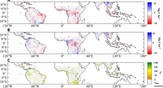
The partial recovery in tropical AGC did not necessarily take place in the same regions that were affected by drought in 2015–2016. To explore this point, we compared the spatial patterns of AGC changes from 2014 to 2015–2016 (AGCEN) and from 2015–2016
Table 1. AGC (Pg) changes over the whole tropics and over tropical regions of Africa, America, and Asia. Changes are given (positive sign for a CO2 land
surface sink) between two periods in time given in the first column (for instance, 2014/2015–2016 corresponds to the change in AGC between year 2014 and the period 2015–2016). As in (17), the range in brackets represents the minimum and maximum of AGC changes estimated by 10 calibrations (see the Supplementary Materials).
Tropics Africa America Asia
2014/2015–2016 [−1.79, −1.37]−1.63 [−1.06, −0.75]−0.91 [−0.80, −0.53]−0.66 [−0.17, −0.00]−0.06 2015–2016/2017 [+0.21, +0.34]+0.30 [−0.06, +0.00]−0.04 [+0.13, +0.23]+0.17 [+0.11, +0.21]+0.17 2016/2017 [+0.66, +1.01]+0.89 [+0.02, 0.12]+0.06 [+0.40, +0.56]+0.50 [+0.24 + 0.40]+0.33 2014/2017 [−1.46, −1.15]−1.33 [−1.09, −0.79]−0.94 [−0.58, −0.37]−0.49 [−0.02, +0.21]+0.11 2010–2017/2017 [−0.64, −0.44]−0.53 [−0.42, −0.28]−0.35 [−0.51, −0.32]−0.43 [+0.16, +0.32]+0.25 on October 27, 2020 http://advances.sciencemag.org/ Downloaded from
to 2017 (AGCR) (Fig. 2, A and B, respectively; subscripts “R” and
“EN” mean “recovery” and “El Niño,” respectively). We found that most tropical regions were affected by AGC losses due to the 2015–2016 El Niño drought. Epicenters of AGC losses (dark red values of AGCEN in Fig. 2A) are located in the eastern Amazon, in central
and southern tropical Africa, and in tropical Asia. Southeastern tropical America and northeastern tropical Asia were less affected by the 2015–2016 El Niño drought. In 2017, a strong recovery (i.e., positive values of AGCR corresponding to blue areas in Fig. 2B)
was found in northern tropical America, in central-western and southern Africa, and in India, but AGC continued to decrease over southern Amazon and Central America and in the central and central-eastern regions of Africa (Fig. 2, A and B).
We defined an AGC recovery ratio by the ratio AGCR/AGCEN
(Fig. 2C). This recovery ratio only accounts for aboveground changes and excludes the soil carbon pool. High-recovery ratios were found in the northernmost parts of tropical America, the western part of the Congo Basin, southern Africa, and central India. These regions generally experienced early recovery dates in 2016 (the date at which the derivative of AGC changed from a negative to a positive sign; see the Supplementary Materials; Fig. 3). We found that from 2015–2016 to 2017, the partial recovery ( + 0.3 +0.2+0.4 Pg C) of tropical AGC stocks (Table 1) accounted only for 18% of the global net land sink recovery (+1.7 Pg C) diagnosed from the global CO2 budget [the value of 1.7 Pg C
includes both natural and land-use change land fluxes computed by considering fossil fuel emissions, to which we subtracted the ocean carbon sink and the growth rate in atmospheric CO2 concentration
(5)]. This suggests either that tropical litter and soil carbon storage increased [as would be expected from increased production of coarse woody debris that have not yet decomposed 1 year after enhanced mortality (21)], which are not measured by L-VOD data, or that an increased northern hemisphere sink (22) contributed to the global land sink recovery. The net tropical sink recovery estimated from four atmospheric inversions (table S1) varies between −0.08 and
+1.04 Pg C [CarboScope-s76, CarboScope-s85, Japan Agency for Marine-Earth Science and Technology (JAMSTEC), and Carbon-Tracker Europe; a higher value of +1.92 Pg C was obtained for Copernicus Atmosphere Monitoring Service (CAMS)]. Hence, atmospheric inversions generally support our results indicating that the recovery of the tropical carbon sink only partly explains the recovery in the global land carbon uptake in 2017 (+1.7 Pg C). Compared to atmospheric inversions, L-VOD–based estimates of AGC values predict a lower contribution of the tropics ( + 0.3 +0.2+0.4 Pg C)
to this global terrestrial carbon uptake. This can be partly explained, as mentioned above, by the fact that the AGC estimates do not account for changes in stocks of coarse woody debris produced in 2015–2016 and changes in soil carbon.
DISCUSSION
The key result of this study is that AGC stocks in the tropics had not recovered from the strong 2015–2016 El Niño event by the end of 2017. This lack of recovery in AGC stocks was revealed relatively to (i) the predrought conditions of 2014 and (ii) the multiyear (2010–2017) AGC average. It was mainly due to decreases in AGC stocks of forests in tropical Africa and tropical America. Notably, humid forests showed weak signs of recovery in America and Asia and showed continuous decline in Africa. Our results point to a large contribution of the African continent to tropical carbon losses during the 2015–2016 El Niño, losses in Africa representing 56% of the −1.6 PgC carbon losses during that event. These results are con-sistent with recent findings obtained from two independent satellite datasets of column CO2 (23). Northern tropical Africa appeared
to be responsible for an unexpectedly large net source of carbon during that period.
Effects from human management on the carbon cycle, in particular the role of tropical deforestation, may affect the results of the study. Our calculations remove the average seasonal cycle of AGC and,
Fig. 2. Spatial patterns of AGC changes corresponding to “El Niño” and “Recovery.” AGC changes (A) from 2014 to 2015–2016 (AGCEN) and (B) from 2015–2016 to
2017 (AGCR) (subscripts “R” and “EN” mean “recovery” and “El Niño,” respectively). In (C), the recovery strength was estimated as the ratio AGCR/AGCEN and expressed
in percentage. AGC stocks were computed from the L-VOD index as described in the Supplementary Materials. Masked pixels (gray) correspond to pixels where no recovery was identified, namely, pixels where either AGCEN > −1 Mg C ha−1 (no losses or very low losses during El Niño 2015–2016) or AGCR < 0 (no recovery in 2017). White areas
correspond to areas where no L-VOD data were available after applying quality flag filtering criteria (see the Supplementary Materials).
on October 27, 2020
http://advances.sciencemag.org/
thus, account for seasonal trends in deforestation activities but not its interannual variability. In Africa, high AGC losses were found in areas where no large-scale deforestation could be detected by monitoring programs, suggesting that either climate conditions or unaccounted deforestation/degradation is the main cause of the AGC stock decreases.
It would be interesting to compare our results to the dynamics of AGC recovery that occurred during former El Niño or drought events. However, this is not straightforward, as no large-scale observational product, comparable to the L-VOD dataset, is currently available to investigate the previous events. Further, each El Niño or drought event and subsequent recovery of vegetation carbon stocks may have a specific signature, both in spatial extent and intensity (9, 24, 25). The continuing decline in AGC stocks in African forests in 2017 may be compared with previous results from the Amazon in relation to the 2005 severe drought that revealed persistent postdrought effects with tree height decreases in the area exposed to severe drought, lagging the precipitation recovery (9, 26). A decline in long-lived components of canopy structure, such as loss of branches or tree falls, can lead to recovery times exceeding 3 to 4 years (9). Further, Yang et al. (26) outlined the persistence of lower carbon biomass stocks even several years after the drought, pointing to linger-ing impacts of droughts on the Amazon forests. In addition, long-term plot records in the Amazon forest suggest a delayed mortality and legacy of carbon emissions after a severe drought (6, 21, 27), which may also apply to other tropical forests. Analysis in (28) linked the California forest die-off during the 2012–2015 drought to delayed mortality effects, namely, mortality, which can be explained by cumula-tive soil moisture depletion. Thus, the forest die-off in California was not attributed to a single extreme dry and warm event in 2015, but rather to a multiyear deep-rooting-zone drought. A similar phe-nomenon could have occurred over the tropics, where the lack of recovery in the carbon stocks in 2017 could also be explained by cumulative soil moisture depletion, related to low precipitation and enhanced evapotranspiration effects, particularly in the northern regions of tropical Africa. The latter regions were affected by successive years of shortage in water storage since 2002 (23). Thus, the hypothesis of delayed mortality effects is consistent with continued negative anomalies in the climatic conditions observed over large tropical areas in 2017 (fig. S6). In 2017, persistent negative anomalies (z scores) for precipitation, surface soil moisture (SM), maximum climatological water deficit [MCWD; an estimate of drought intensity and a correlate of forest tree mortality (6, 24)], and the cumulative P − ET deficit, combined with positive anomalies for land surface temperature and vapor pressure deficit (VPD) were observed in tropical America and central and eastern tropical Africa (fig. S6, C to H). The spatial patterns of the anomalies in AGC are in good agreement with those derived independently from other remote sensing vegetation indices, such as the enhanced vegetation index (EVI) and solar-induced chlorophyll
fluorescence (SIF) (fig. S6, B and I). Northwestern and northeastern regions of tropical Africa showing low recovery (fig. S2B) and negative anomalies (fig. S6A) in the AGC stocks in 2017 coincide with those revealed from satellite-based record of column CO2 from
2009 onward (23). These regions also showed precipitation and cumulative soil moisture deficits, as estimated by the cumulative P − ET values (fig. S1G). Generally, the largest loci found in (23) of (i) carbon emissions in the northern regions of tropical Africa, in the central-eastern regions in tropical America, and in the Borneo island, and of (ii) carbon sinks in the western and southern regions of tropical America, the Congo Basin, and the northern regions of tropical Asia are also quite consistent with our results (fig. S1A). Notably, anomalies in climate variables consistent with low drought stress are predominantly found over tropical Asia and explain the AGC stock recovery in this region.
Our AGC estimates based on L-band microwave observations feature low saturation effects up to AGC levels of ~200 tC ha−1 (fig. S1) (16, 17). However, it cannot be excluded that saturation effects may affect some AGC estimates at very high biomass levels (>200 tC ha−1) that can be found mainly in the moist tropical forests of the Amazon and Congo Basins. Also, the spatial resolution of the space-borne L-VOD observations limits the ability of L-VOD to accurately attribute C stock changes to climate and/or anthropogenic drivers. However, L-VOD integrates the impact of this range of drivers, providing direct estimates of C stocks and, thus, key inputs for the GCB. These integrated estimates of changes in AGC could be valuable to carry out large-scale validation of other products associated specifically with different aspects of the tropical carbon budget [for instance, mapping and evaluating the impacts of C stocks from fires and deforestation (29, 30) and associated regrowth processes (31)].
Our results demonstrate how the L-VOD dataset, retrieved from passive L-band observations, supports the assessment of the tropical forest carbon balance (32), and the study confirms the high-value L-VOD to monitor the impact of large climate anomalies on the terrestrial C-stock in near real time. In particular, our findings show that soil moisture depletion associated with El Niño events in large tropical regions followed ongoing drought events, leading to enhanced cumula-tive P − ET decline, and important carbon stock losses as revealed here especially in tropical Africa. These findings have important im-plications for the long-term vulnerability of carbons stocks in the tropics, as large-scale droughts and El Niño events are expected to intensify, in terms of both frequency and intensity (33), and their suc-cession may have marked cumulative effects on deep-rooting-zone drying and, consequently, on AGC stock losses. Thus, the L-VOD data provide unique large-scale observations of changes in vegetation carbon stocks at a critical time where improved understanding of the impacts of climate change on ecosystems is essential. So, ensuring continuity in the long-term records of these observations is important, but next-generation spatial missions have not yet been decided.
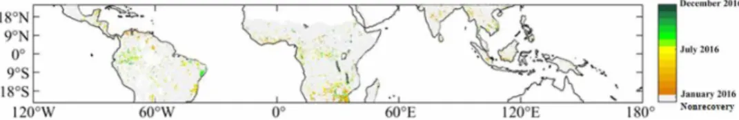
Fig. 3. Map of the AGC “recovery” date. The date was defined here as the date of the minimum value in the AGC stocks over year 2016. To ensure that this date corresponded well to a minimum (the inflexion point in the AGC anomaly curve), we excluded recovery dates at the very beginning or at the very end of 2016. Gray and white areas are defined in the caption of Fig. 2. An estimate of the uncertainty value associated with the recovery date is presented in the Supplementary Materials.
on October 27, 2020
http://advances.sciencemag.org/
MATERIALS AND METHODS Land cover and humidity classes
Land cover types were derived from the IGBP (International Geosphere-Biosphere Programme) scheme of land cover classifica-tion for 2015 (34). The IGBP scheme considers 17 cover types (fig. S3). The data were aggregated to 25-km resolution by dominant class within each SMOS L-VOD grid cell. “Dominant” refers to the class that has the largest number of 500-m native resolution pixels within each SMOS grid cell. We used the 500-m Moderate Resolu-tion Imaging Spectroradiometer (MODIS)–based global land cover climatology map based on 10 years (2001–2010) of the MODIS MCD12Q1 product, which contains land cover information.
We merged the original IGBP classes to reduce the number of classes to three biomes (forests, shrublands and savannas, and grasslands and croplands), sorted by potentially decreasing woody cover and carbon density. Forests include IGBP classes 1 to 5 (ever-green needleleaf forest, ever(ever-green broadleaf forest, deciduous needle-leaf forest, deciduous broadneedle-leaf forest, and mixed forest); shrublands and savannas include IGBP classes 6 to 9 (closed and open shrublands, woody savannas, and savannas); and grasslands and croplands include classes 10, 12, and 14 (grasslands, croplands, and cropland/ natural vegetation mosaics).
The deforested and nondeforested areas in the tropics were defined on the basis of the forest area loss map produced by (20). Pixels with more than 5% forest losses (covering 16% of the tropics) are considered to correspond to deforested areas. Forest percentage loss rates during the study period of 2014–2017 were calculated at the resolution of SMOS as the proportion of the summed areas of forest loss (detected by the “yearloss” map) within each SMOS grid cell (~25 km).
We masked the nonvegetated SMOS pixels, where SMOS re-trievals of L-VOD and SM do not apply, dominated by “wetland,” “urban and built-up,” “snow and ice,” “water,” and “barren or sparsely vegetated,” based on the aggregated 25-km IGBP land cover map. The map of drylands versus humid regions was defined using the aridity index (AI) corresponding to the ratio between annual pre-cipitation and total annual potential evapotranspiration (16, 17, 18), with drylands having an AI lower than 0.65 as proposed by the United Nations Environment Programme (UNEP). This map was later referred to as the UNEP map. To evaluate the sensitivity of the results shown in fig. S2 to the ratio of 0.65, we applied a different map separating drylands and humid regions. This second map was computed from a global AI (GAI), which is calculated as the ratio of precipitation to potential evapotranspiration (P/PET) and is provided by the GAI and Potential Evapotranspiration (ET0) Climate Data-base v2, where drylands are defined by GAI ≤0.65 (35). This map is referred to as the GAI map. We changed the threshold of the GAI map up and down by 5% threshold intervals, and five different thresholds values (0.59, 0.62, 0.65, 0.68, and 0.72) were tested to define new maps of drylands. On the basis of these new maps, we computed AGC anomalies and compared them to results given in fig. S2 based on the UNEP map.
The new results based on the GAI maps for the different threshold values are shown in fig. S7. It can be seen that (i) results obtained with the GAI and UNEP maps are very similar, and (ii) there is a rather low sensitivity of the results to the threshold values used to define drylands in the GAI maps. A larger sensitivity of the results to the threshold value was found in tropical Asia at the end of 2017, with a low impact on the main conclusions of this study.
Vegetation and climate variables
To evaluate the impact of the drought stress on the carbon uptake by plants, we used several vegetation indexes and climate variables (fig. S6):
1) MEI (18)
2) Precipitation at a spatial resolution of 0.25° from datasets of the Tropical Rainfall Measuring Mission (TRMM 3B43 v7) from 1998 to 2017 (36)
3) MCWD [an estimate of drought intensity at a spatial resolu-tion of 0.25° calculated from TRMM precipitaresolu-tion (37)]
4) SM obtained, as for L-VOD, from the SMOS-IC product, V105 (16, 17, 38), from 2010 to 2017. The multiangular and dual- polarization SMOS observations ensure a good decoupling between the effects of soil moisture and vegetation, parameterized here by the L-VOD index (15, 17). SMOS-IC SM has been recently evaluated with other recently reprocessed global SM products against in situ International Soil Moisture Network (ISMN) datasets and performs very well (39, 40); in (40), it was found to be the most performant remote sensing SM product in dense vegetation conditions
5) Land surface temperature at a spatial resolution of 0.25° obtained from skin temperature data produced by the European Centre for Medium-Range Weather Forecasts (ECMWF) atmospheric reanalysis ERA-Interim during 1979 and 2017 (38)
6) VPD at a spatial resolution of 1° from 2002 to 2017, calculated using near-surface air temperature and surface relative humidity from both the daytime and nighttime overpasses (1:30 p.m. and 1:30 a.m., respectively) of the Atmospheric Infrared Sounder (version 6) (41)
7) Cumulative water balance was computed by cumulating precip-itation minus evapotranspiration (P − ET, mm) starting 1 January 2010, as for the L-VOD time series analyzed in this study. Precipitation was estimated as defined above from the TRMM 3B43 v7 data. Evapo-transpiration was obtained from the GLEAM v3 satellite- based dataset (42). As in (17), the spatial patterns of the anomalies in AGC were compared with those derived independently from other re-mote sensing vegetation indices, such as the EVI and SIF. The EVI was obtained from the monthly MODIS Vegetation Index product (MOD13C2 Climate Modeling Grid) at a spatial resolution of 0.05° from 2010 to 2017. SIF was obtained from version 27 global monthly (level 3) product at a spatial resolution of 0.5° from 2007 to 2017 retrieved from the Global Ozone Monitoring Experiment 2 (GOME-2) instrument.
Precipitation, land surface temperature, EVI, and SIF were aggre-gated to an annual composite at 25 -km spatial resolution by averag-ing or bilinear interpolation from their original resolution to match the L-VOD grid. In fig. S6, yearly anomalies were calculated using the z score: (value − mean)/SD.
Benchmark maps of AGC density
Brandt et al. (16) have used the maps produced by Baccini et al. (43) for calibrating the L-VOD/AGC relationship for Africa. Here, as in (17), we used four static AGC benchmark maps (fig. S1) to calibrate L-VOD and retrieve AGC to decrease the dependence of our results on the accuracy of a single biomass map. These maps include three pantropical maps published by (43, 44, 45), hereafter referred to as the “Saatchi,” “Avitabile,” and “Baccini” maps, respectively. The Saatchi map used in the present study is an updated version, which represents AGC circa 2015 (46). A fourth map covering only Africa and hereinafter referred to as the “Bouvet-Mermoz” map was used (17). The original units of aboveground biomass density (Mg ha−1)
on October 27, 2020
http://advances.sciencemag.org/
were converted to AGC density (Mg C ha−1) by multiplying the original values by a factor of 0.5 (16). All AGC maps were aggregated to 25-km spatial resolution to match the spatial resolution of the SMOS data by averaging AGC pixels within the SMOS grid cells. Retrieved AGC products and uncertainty associated with the AGC estimates
As in (16, 17), changes in AGC were estimated from the L-VOD pro-duct using SMOS datasets in the newly developed SMOS-IC version (38). In the SMOS-IC algorithm, L-VOD and SM are retrieved simul-taneously without external vegetation or hydrologic products as in-puts in the L-band microwave emission of the biosphere inversion model. L-VOD retrievals, thus, depend only on temperature fields from the ECMWF for calculating the effective surface temperature and are independent of any vegetation index. This improvement makes this new product very robust for applications in ecology and climate change studies (3, 16, 17).
The root mean square error (RMSE) between the measured and simulated brightness temperature (referred to as RMSE-TB) associated with the SMOS-IC product was used to filter out observations affected by radio frequency interference (RFI), which perturbs the natural microwave emission from Earth surface measured by passive micro-wave systems. We excluded daily observations, influenced by RFI effects, for which RMSE-TB was larger than 6 K (38). Robust estimates of annual L-VOD and SM were then obtained as the medians of all high-quality ascending and descending retrievals with more than 30 valid observations per year. This filtering left a large fraction of the original SMOS pixels available for the analysis in tropical biomes over America (74%), Africa (94%), and Asia (72%).
Over woody vegetation, L-VOD is mainly sensitive to the vegeta-tion water content (VWC) of stems and branches (kg/m2) (15), which can be computed from the values of biomass and of the moisture content of vegetation (Mg, %). Assuming that the yearly average of Mg is relatively constant between years at the spatial scale of the SMOS grid (25 km × 25 km), yearly average values of VWC and biomass are strongly correlated over time. This explains that several studies have reported a strong relationship between L-VOD and biomass for woody vegetation, which is almost linear and independent of the year of calculation (16, 17). The yearly average of L-VOD, through its strong link to VWC, can thus be considered as a robust proxy of biomass.
The method used here to compute AGC from L-VOD is the same as the one used in (17), where it is described in detail. The L-VOD dataset allows computation of annual AGC values at a resolution of 25 km, but these values cannot be validated directly, as no other dataset has this capability to date. So, indirect validation of the L-VOD–derived AGC values has been made in (16, 17) against numerous datasets evaluating changes in forest area, spatial patterns of greening/browning trends computed from optical remote sensing observations, climate variables, and atmospheric modeling of carbon sinks and sources in the tropics. An extensive analysis of the un-certainties associated with the L-VOD–derived AGC estimates has been made as well in the Supplementary Materials of (17), and rela-tive uncertainties associated with changes in the carbon stocks over the tropics have been estimated to be in the order of 20 to 25% (for instance, this corresponds to an uncertainty of 0.15 Pg C for estimated changes in the carbon stocks of 0.66 Pg C over the tropics). We will not duplicate these analyses in this study, and we refer the readers to (17) on the questions related to uncertainties and validation of the
AGC values computed from the new SMOS-IC L-VOD satellite data. However, for a better understanding of the use of the new L-VOD dataset, the main steps of the computation of the AGC values as detailed in (17) are given in the following.
The yearly L-VOD data were ranked from low to high VOD values and were pooled into bins of 250 grid cells as in (47). The mean of the corresponding AGC distribution in the reference map was calculated for each L-VOD bin to obtain an AGC curve as a function of L-VOD. The curve was fitted using the four-parameter function (47)
AGC = a × arctan(b × (VOD − c ) ) − arctan(− b × c) ─────────────────────── arctan(b × (Inf − c ) ) − arctan(− b × c) + d (1)
where a, b, c, and d are four best-fit parameters (table S2) and VOD is the yearly L-VOD data. As in (16, 17), we used here the year 2011 (the year used for calibration proved to have very little impact on the calibrated curves). An illustration of the calibrated relationships between L-VOD and AGC based on the Saatchi, Baccini, Avitabile, and Bouvet-Mermoz maps is given in fig. S1. We converted the yearly L-VOD map into maps of yearly AGC density (Mg C ha−1) for 2010–2017 using Eq. 1. Regional AGC stocks were obtained by multiplying the AGC density by the area of the corresponding L-VOD pixels.
AGC benchmark maps contain uncertainties and bias, and no single map can be considered fully reliable, as outlined above. We used all the different maps to fit Eq. 1 for tropical America, tropical Africa, and the entire tropical region separately. Benchmark maps in tropical Asia were not used in this calibration process due to the limited number of SMOS observations in the region. Ten calibrations of Eq. 1 were thereby obtained (table S2). We used all 10 calibrations to create 10 maps of AGC stocks. We used the median of these 10 maps to calculate yearly tropical AGC maps during 2010–2017. The minima and maxima were also reported, as they provide esti-mates of the uncertainty of retrieved AGC estiesti-mates used in this study that relates to systematic errors in the reference biomass maps. Anomalies of AGC stocks computed from the L-VOD index The AGC anomalies (Fig. 1) at the continental scale were computed by summing the deseasonalized AGC anomalies estimated separately over each pixel and were smoothed using a sliding-window average (T = 120 days). To compute the deseasonalized AGC anomalies at the pixel scale, we estimated the time series of AGC to which we removed the average seasonal cycle of AGC computed over 2010–2017 for each pixel. AGC stocks were computed from the L-VOD index as follows: daily ascending/descending L-VOD data with an RMSE-TB larger than 6 K and the 10th/90th outliers were filtered out (L-VOD values for days with overlapped ascending/descending L-VOD data were averaged). A sliding-window average (T = 90 days) was used to smooth the times series at the pixel scale.
Recovery date
The AGC recovery date (Fig. 3) was computed for each pixel as the date of the minimum value of AGC stocks during 2017, correspond-ing to the inflexion point in the AGC anomaly curve. To ensure that this date corresponded well to an inflexion point in the AGC anomaly curve, we excluded recovery dates at the very beginning or at the very end of 2017. Over short (daily or weekly) time scales, changes in the L-VOD parameter are mainly sensitive to changes in the water
on October 27, 2020
http://advances.sciencemag.org/
content of the whole vegetation layer (15), so that the link with changes in C stocks are indirect. However, it is very likely that the recovery in the vegetation water status, after a long drought period, can be associated with a recovery in vegetation productivity and C stocks.
To obtain an estimate of the uncertainty value associated with the recovery date, we evaluated for each pixel the range of days corre-sponding to AGC anomaly values lower than Min + TH, where Min
is the value of the minimum AGC value for the pixel and TH is a fixed
threshold value. We selected a value of TH = 0.1 Mg C ha−1
corre-sponding to ~4% of the average value of the minimum AGC anomaly (−2.65 Mg C ha−1) for the pixels.
In summary, we computed for each pixel the range of days sur-rounding the recovery date and corresponding to an AGC anomaly < Min + 0.1 Tg C. A narrow range of days will correspond to a low uncertainty associated with the date of recovery (AGC anomaly curve with a minimum defined by a “sharp drop”). A large range of days will correspond to a high uncertainty associated with the date of recovery (AGC anomaly curve with a minimum defined by a “smooth valley”). The map of the per-pixel uncertainty value associated with the recovery (as defined by the range of days surrounding the recovery date and computed as described above) is given in fig. S8. The average value of this range of days is ±25 days (SD = ±21 days) and provides a reasonable estimate of the average uncertainty associated with the recovery date.
Atmospheric data and inversions
Five observation-based datasets of net land-atmosphere surface fluxes were used to compute the land sink (Pg C) and land sink recovery (Pg C) from model inversion over the tropics: the CAMS atmospheric inversion version 16r1 (48), the Jena CarboScope inversion versions s76_v4.1 and s85 (49), JAMSTEC (50), and CarbonTracker Europe (CTE) (51). More details about the differences in model inversions of CAMS, Jena CarboScope, and JAMSTEC are given in (5).
The CAMS data (Copernicus service) are available from ECMWF. The CTE data are available at www.carbontracker.eu/fluxtimeseries. php. The JAMSTEC data were obtained upon request from P. Patra (JAMSTEC). For the five atmospheric inversions, the land sink recovery was computed as the average of the land sink over 2017 minus that over 2015–2016 (table S1).
SUPPLEMENTARY MATERIALS
Supplementary material for this article is available at http://advances.sciencemag.org/cgi/ content/full/6/6/eaay4603/DC1
Fig. S1. Scatterplots between yearly mean L-VOD in 2011 and benchmark AGC density maps. Fig. S2. Anomaly of the P − ET deficit (mm) superimposed on the anomalies of AGC stocks estimated from the L-VOD index in the tropics.
Fig. S3. Biome classes for 2001 to 2010 based on the MODIS IGBP products over the tropics. Fig. S4. Anomalies of AGC stocks estimated from the L-VOD index in tropical regions. Fig. S5. Map of deforested and nondeforested areas over the tropics.
Fig. S6. The 2017 anomalies in remote sensing indices and climate variables.
Fig. S7. Anomalies in the P − ET deficit (mm) and in AGC stocks considering different maps of drylands and humid areas.
Fig. S8. Map of the uncertainty value associated with the recovery date.
Table S1. Land sink (Pg C) and land sink recovery (Pg C) computed from model inversion over the tropics.
Table S2. Fitted parameters (a, b, c, and d) in Eq. 1 in the Supplementary Materials for the relationship between L-VOD in 2011 and AGC.
REFERENCES AND NOTES
1. J. Liu, K. W. Bowman, D. S. Schimel, N. C. Parazoo, Z. Jiang, M. Lee, A. A. Bloom, D. Wunch, C. Frankenberg, Y. Sun, C. W. O’Dell, K. R. Gurney, D. Menemenlis, M. Gierach, D. Crisp, A. Eldering, Contrasting carbon cycle responses of the tropical continents to the 2015–2016 El Niño. Science 358, eaam5690 (2017).
2. J. C. Jiménez-Muñoz, C. Mattar, J. Barichivich, A. Santamaría-Artigas, K. Takahashi, Y. Malhi, J. A. Sobrino, G. Van Der Schrier, Record-breaking warming and extreme drought in the Amazon rainforest during the course of El Niño 2015–2016. Sci. Rep. 6, 33130 (2016).
3. A. Bastos, P. Friedlingstein, S. Sitch, C. Chen, A. Mialon, J.-P. Wigneron, V. K. Arora, P. R. Briggs, J. G. Canadell, P. Ciais, F. Chevallier, L. Cheng, C. Delire, V. Haverd, A. K. Jain, F. Joos, E. Kato, S. Lienert, D. Lombardozzi, J. R. Melton, R. Myneni, J. E. M. S. Nabel, J. Pongratz, B. Poulter, C. Rödenbeck, R. Séférian, H. Tian, C. van Eck, N. Viovy, N. Vuichard, A. P. Walker, A. Wiltshire, J. Yang, S. Zaehle, N. Zeng, D. Zhu, Impact of the 2015/2016 El Niño on the terrestrial carbon cycle constrained by bottom-up and top-down approaches. Philos. Trans. R. Soc. Lond. Ser. B Biol. Sci. 373, 20170304 (2018).
4. C. Yue, P. Ciais, A. Bastos, F. Chevallier, Y. Yin, C. Rödenbeck, T. Park, Vegetation greenness and land carbon-flux anomalies associated with climate variations: A focus on the year 2015. Atmos. Chem. Phys. 17, 13903–13919 (2017).
5. C. Le Quéré, R. M. Andrew, P. Friedlingstein, S. Sitch, J. Pongratz, A. C. Manning, J. I. Korsbakken, G. P. Peters, J. G. Canadell, R. B. Jackson, T. A. Boden, P. P. Tans, O. D. Andrews, V. K. Arora, D. C. E. Bakker, L. Barbero, M. Becker, R. A. Betts, L. Bopp, F. Chevallier, L. P. Chini, P. Ciais, C. E. Cosca, J. Cross, K. Currie, T. Gasser, I. Harris, J. Hauck, V. Haverd, R. A. Houghton, C. W. Hunt, G. Hurtt, T. Ilyina, A. K. Jain, E. Kato, M. Kautz, R. F. Keeling, K. Klein Goldewijk, A. Körtzinger, P. Landschützer, N. Lefèvre, A. Lenton, S. Lienert, I. Lima, D. Lombardozzi, N. Metzl, F. Millero, P. M. S. Monteiro, D. R. Munro, J. E. M. S. Nabel, S. I. Nakaoka, Y. Nojiri, X. A. Padin, A. Peregon, B. Pfeil, D. Pierrot, B. Poulter, G. Rehder, J. Reimer, C. Rödenbeck, J. Schwinger, R. Séférian, I. Skjelvan, B. D. Stocker, H. Tian, B. Tilbrook, F. N. Tubiello, I. T. van der Laan-Luijkx, G. R. van der Werf, S. van Heuven, N. Viovy, N. Vuichard, A. P. Walker, A. J. Watson, A. J. Wiltshire, S. Zaehle, D. Zhu, Global Carbon Budget 2017. Earth Syst. Sci. Data 10, 405–448 (2018).
6. O. L. Phillips, L. E. O. C. Aragão, S. L. Lewis, J. B. Fisher, J. Lloyd, G. López-González, Y. Malhi, A. Monteagudo, J. Peacock, C. A. Quesada, G. van der Heijden, S. Almeida, I. Amaral, L. Arroyo, G. Aymard, T. R. Baker, O. Bánki, L. Blanc, D. Bonal, P. Brando, J. Chave, Á. C. A. de Oliveira, N. D. Cardozo, C. I. Czimczik, T. R. Feldpausch, M. A. Freitas, E. Gloor, N. Higuchi, E. Jiménez, G. Lloyd, P. Meir, C. Mendoza, A. Morel, D. A. Neill, D. Nepstad, S. Patiño, M. C. Peñuela, A. Prieto, F. Ramírez, M. Schwarz, J. Silva, M. Silveira, A. S. Thomas, H. T. Steege, J. Stropp, R. Vásquez, P. Zelazowski, E. A. Dávila, S. Andelman, A. Andrade, K.-J. Chao, T. Erwin, A. Di Fiore, E. C. Honorio, H. Keeling, T. J. Killeen, W. F. Laurance, A. P. Cruz, N. C. A. Pitman, P. N. Vargas, H. Ramírez-Angulo, A. Rudas, R. Salamão, N. Silva, J. Terborgh, A. Torres-Lezama, Drought Sensitivity of the Amazon Rainforest. Science 323, 1344–1347 (2009).
7. R. J. W. Brienen, O. L. Phillips, T. R. Feldpausch, E. Gloor, T. R. Baker, J. Lloyd, G. Lopez-Gonzalez, A. Monteagudo-Mendoza, Y. Malhi, S. L. Lewis, R. Vásquez Martinez, M. Alexiades, E. Álvarez Dávila, P. Alvarez-Loayza, A. Andrade, L. E. O. C. Aragão, A. Araujo-Murakami, E. J. M. M. Arets, L. Arroyo, C. G. A. Aymard, O. S. Bánki, C. Baraloto, J. Barroso, D. Bonal, R. G. A. Boot, J. L. C. Camargo, C. V. Castilho, V. Chama, K. J. Chao, J. Chave, J. A. Comiskey, F. C. Valverde, L. da Costa, E. A. de Oliveira, A. Di Fiore, T. L. Erwin, S. Fauset, M. Forsthofer, D. R. Galbraith, E. S. Grahame, N. Groot, B. Hérault, N. Higuchi, E. N. Honorio Coronado, H. Keeling, T. J. Killeen, W. F. Laurance, S. Laurance, J. Licona, W. E. Magnussen, B. S. Marimon, B. H. Marimon-Junior, C. Mendoza, D. A. Neill, E. M. Nogueira, P. Núñez, N. C. Pallqui Camacho, A. Parada, G. Pardo-Molina, J. Peacock, M. Peña-Claros, G. C. Pickavance, N. C. A. Pitman, L. Poorter, A. Prieto, C. A. Quesada, F. Ramírez, H. Ramírez-Angulo, Z. Restrepo, A. Roopsind, A. Rudas, R. P. Salomão, M. Schwarz, N. Silva, J. E. Silva-Espejo, M. Silveira, J. Stropp, J. Talbot, H. ter Steege, J. Teran-Aguilar, J. Terborgh, R. Thomas-Caesar, M. Toledo, M. Torello-Raventos, R. K. Umetsu, G. M. F. van der Heijden, P. van der Hout, I. C. Guimarães Vieira, S. A. Vieira, E. Vilanova, V. A. Vos, R. J. Zagt, Long-term decline of the Amazon carbon sink. Nature 519, 344 (2015).
8. J. Verbesselt, N. Umlauf, M. Hirota, M. Holmgren, E. H. Van Nes, M. Herold, A. Zeileis, M. Scheffer, Remotely sensed resilience of tropical forests. Nat. Clim. Chang. 6, 1028–1031 (2016).
9. S. Saatchi, S. Asefi-Najafabady, Y. Malhi, L. E. O. C. Aragão, L. O. Anderson, R. B. Myneni, R. Nemani, Persistent effects of a severe drought on Amazonian forest canopy.
Proc. Natl. Acad. Sci. U.S.A. 110, 565–570 (2013).
10. D. C. Zemp, C.-F. Schleussner, H. M. J. Barbosa, M. Hirota, V. Montade, G. Sampaio, A. Staal, L. Wang-Erlandsson, A. Rammig, Self-amplified Amazon forest loss due to vegetation-atmosphere feedbacks. Nat. Commun. 8, 14681 (2017).
11. A. Ahlström, M. R. Raupach, G. Schurgers, B. Smith, A. Arneth, M. Jung, M. Reichstein, J. G. Canadell, P. Friedlingstein, A. K. Jain, E. Kato, B. Poulter, S. Sitch, B. D. Stocker, N. Viovy, Y. P. Wang, A. Wiltshire, S. Zaehle, N. Zeng, The dominant role of semi-arid ecosystems in the trend and variability of the land CO2 sink. Science 348, 895–899 (2015).
12. G. P. Peters, C. Le Quéré, R. M. Andrew, J. G. Canadell, P. Friedlingstein, T. Ilyina, R. B. Jackson, F. Joos, J. I. Korsbakken, G. A. McKinley, S. Sitch, P. Tans, Towards real-time verification of CO2 emissions. Nat. Clim. Chang. 7, 848–850 (2017).
on October 27, 2020
http://advances.sciencemag.org/
13. W. A. Kurz, C. C. Dymond, G. Stinson, G. J. Rampley, E. T. Neilson, A. L. Carroll, T. Ebata, L. Safranyik, Mountain pine beetle and forest carbon feedback to climate change. Nature 452, 987–990 (2008).
14. C. D. Allen, D. D. Breshears, N. G. McDowell, On underestimation of global vulnerability to tree mortality and forest die-off from hotter drought in the Anthropocene. Ecosphere 6, 1–55 (2015).
15. J.-P. Wigneron, T. J. Jackson, P. O’Neill, G. De Lannoy, P. de Rosnay, J. P. Walker, P. Ferrazzoli, V. Mironov, S. Bircher, J. P. Grant, M. Kurum, M. Schwank, J. Munoz-Sabater, N. Das, A. Royer, A. Al-Yaari, A. Al Bitar, R. Fernandez-Moran, H. Lawrence, A. Mialon, M. Parrens, P. Richaume, S. Delwart, Y. Kerr, Modelling the passive microwave signature from land surfaces: A review of recent results and application to the L-band SMOS & SMAP soil moisture retrieval algorithms. Remote Sens. Environ. 192, 238–262 (2017). 16. M. Brandt, J.-P. Wigneron, J. Chave, T. Tagesson, J. Penuelas, P. Ciais, K. Rasmussen,
F. Tian, C. Mbow, A. Al-Yaari, N. Rodriguez-Fernandez, G. Schurgers, W. Zhang, J. Chang, Y. Kerr, A. Verger, C. Tucker, A. Mialon, L. V. Rasmussen, L. V. Fan, R. Fensholt, Satellite passive microwaves reveal recent climate-induced carbon losses in African drylands.
Nat. Ecol. Evol. 2, 827–835 (2018).
17. L. Fan, J.-P. Wigneron, P. Ciais, J. Chave, M. Brandt, R. Fensholt, S. S. Saatchi, A. Bastos, A. Al-Yaari, K. Hufkens, Y. Qin, X. Xiao, C. Chen, R. B. Myneni, R. Fernandez-Moran, A. Mialon, N. J. Rodriguez-Fernandez, Y. Kerr, F. Tian, J. Penuelas, Satellite observed pantropical carbon dynamics. Nat. Plants 5, 944–951 (2019).
18. K. Wolter, M. S. Timlin, El Niño/Southern Oscillation behaviour since 1871 as diagnosed in an extended multivariate ENSO index (MEI.ext). Int. J. Climatol. 31, 1074–1087 (2011). 19. J.-F. Bastin, N. Berrahmouni, A. Grainger, D. Maniatis, D. Mollicone, R. Moore, C. Patriarca,
N. Picard, B. Sparrow, E. M. Abraham, K. Aloui, A. Atesoglu, F. Attore, Ç. Bassüllü, A. Bey, M. Garzuglia, L. G. García-Montero, N. Groot, G. Guerin, L. Laestadius, A. J. Lowe, B. Mamane, G. Marchi, P. Patterson, M. Rezende, S. Ricci, I. Salcedo, A. S.-P. Diaz, F. Stolle, V. Surappaeva, R. Castro, The extent of forest in dryland biomes. Science 356, 635–638 (2017).
20. M. C. Hansen, P. V. Potapov, R. Moore, M. Hancher, S. A. Turubanova, A. Tyukavina, D. Thau, S. V. Stehman, S. J. Goetz, T. R. Loveland, A. Kommareddy, A. Egorov, L. Chini, C. O. Justice, J. R. G. Townshend, High-Resolution Global Maps of 21st-Century Forest Cover Change. Science 342, 850–853 (2013).
21. N. Ramankutty, H. K. Gibbs, F. Achard, R. Defries, J. A. Foley, R. A. Houghton, Challenges to estimating carbon emissions from tropical deforestation. Glob. Chang. Biol. 13, 51–66 (2007).
22. Y. Pan, R. A. Birdsey, J. Fang, R. Houghton, P. E. Kauppi, W. A. Kurz, O. L. Phillips, A. Shvidenko, S. L. Lewis, J. G. Canadell, P. Ciais, R. B. Jackson, S. W. Pacala, A. D. McGuire, S. Piao, A. Rautiainen, S. Sitch, D. Hayes, A Large and Persistent Carbon Sink in the World’s Forests. Science 333, 988–993 (2011).
23. P. I. Palmer, L. Feng, D. Baker, F. Chevallier, H. Bösch, P. Somkuti, Net carbon emissions from African biosphere dominate pan-tropical atmospheric CO2 signal. Nat. Commun. 10, 3344 (2019).
24. S. L. Lewis, P. M. Brando, O. L. Phillips, G. M. van der Heijden, D. Nepstad, The 2010 amazon drought. Science 331, 554 (2011).
25. B. Poulter, D. Frank, P. Ciais, R. B. Myneni, N. Andela, J. Bi, G. Broquet, J. G. Canadell, F. Chevallier, Y. Y. Liu, S. W. Running, S. Sitch, G. R. van der Werf, Contribution of semi-arid ecosystems to interannual variability of the global carbon cycle. Nature 509, 600 (2014). 26. Y. Yang, S. S. Saatchi, L. Xu, Y. Yu, S. Choi, N. Phillips, R. Kennedy, M. Keller, Y. Knyazikhin, R. B. Myneni, Post-drought decline of the Amazon carbon sink. Nat. Commun. 9, 3172 (2018).
27. R. Condit, S. P. Hubbell, R. B. Foster, Mortality rates of 205 neotropical tree and shrub species and the impact of a severe drought. Ecol. Monogr. 65, 419–439 (1995). 28. M. L. Goulden, R. C. Bales, California forest die-off linked to multi-year deep soil drying
in 2012–2015 drought. Nat. Geosci. 12, 632–637 (2019).
29. S. Zhou, Y. Zhang, A. Park Williams, P. Gentine, Projected increases in intensity, frequency, and terrestrial carbon costs of compound drought and aridity events. Sci. Adv. 5, eaau5740 (2019).
30. A. Baccini, W. Walker, L. Carvalho, M. Farina, D. Sulla-Menashe, R. A. Houghton, Tropical forests are a net carbon source based on aboveground measurements of gain and loss.
Science 358, 230–234 (2017).
31. R. L. Chazdon, E. N. Broadbent, D. M. A. Rozendaal, F. Bongers, A. M. A. Zambrano, T. M. Aide, P. Balvanera, J. M. Becknell, V. Boukili, P. H. S. Brancalion, D. Craven, J. S. Almeida-Cortez, G. A. L. Cabral, B. de Jong, J. S. Denslow, D. H. Dent, S. J. DeWalt, J. M. Dupuy, S. M. Durán, M. M. Espírito-Santo, M. C. Fandino, R. G. César, J. S. Hall, J. L. Hernández-Stefanoni, C. C. Jakovac, A. B. Junqueira, D. Kennard, S. G. Letcher, M. Lohbeck, M. Martínez-Ramos, P. Massoca, J. A. Meave, R. Mesquita, F. Mora, R. Muñoz, R. Muscarella, Y. R. F. Nunes, S. Ochoa-Gaona, E. Orihuela-Belmonte, M. Peña-Claros, E. A. Pérez-García, D. Piotto, J. S. Powers, J. Rodríguez-Velazquez, I. E. Romero-Pérez, J. Ruíz, J. G. Saldarriaga, A. Sanchez-Azofeifa, N. B. Schwartz, M. K. Steininger, N. G. Swenson, M. Uriarte, M. van Breugel, H. van der Wal, M. D. M. Veloso, H. Vester, I. C. G. Vieira, T. V. Bentos, G. B. Williamson, L. Poorter, Carbon sequestration potential
of second-growth forest regeneration in the Latin American tropics. Sci. Adv. 2, e1501639 (2016).
32. E. T. A. Mitchard, The tropical forest carbon cycle and climate change. Nature 559, 527–534 (2018).
33. V. H. Dale, L. A. Joyce, S. McNulty, R. P. Neilson, M. P. Ayres, M. D. Flannigan, P. J. Hanson, L. C. Irland, A. E. Lugo, C. J. Peterson, D. Simberloff, F. J. Swanson, B. J. Stocks, B. M. Wotton, Climate change and forest disturbances: Climate change can affect forests by altering the frequency, intensity, duration, and timing of fire, drought, introduced species, insect and pathogen outbreaks, hurricanes, windstorms, ice storms, or landslides. Bioscience 51, 723–734 (2001).
34. P. D. Broxton, X. Zeng, D. Sulla-Menashe, P. A. Troch, A Global Land Cover Climatology Using MODIS Data. J. Appl. Meteorol. Climatol. 53, 1593–1605 (2014).
35. A. Trabucco, R. Zomer, Global Aridity Index and Potential Evapotranspiration (ET0) Climate Database v2. figshare. Fileset (2019); https://doi.org/10.6084/m9. figshare.7504448.v3.
36. G. J. Huffman, D. T. Bolvin, E. J. Nelkin, D. B. Wolff, R. F. Adler, G. Gu, Y. Hong, K. P. Bowman, E. F. Stocker, The TRMM Multisatellite Precipitation Analysis (TMPA): Quasi-Global, Multiyear, Combined-Sensor Precipitation Estimates at Fine Scales.
J. Hydrometeorol. 8, 38–55 (2007).
37. L. E. O. C. Aragão, Y. Malhi, R. M. Roman-Cuesta, S. Saatchi, L. O. Anderson, Y. E. Shimabukuro, Spatial patterns and fire response of recent Amazonian droughts.
Geophys. Res. Lett. 34, L07701 (2007).
38. R. Fernandez-Moran, A. Al-Yaari, A. Mialon, A. Mahmoodi, A. Al Bitar, G. De Lannoy, N. Rodriguez-Fernandez, E. Lopez-Baeza, Y. Kerr, J.-P. Wigneron, SMOS-IC: An alternative SMOS soil moisture and vegetation optical depth product. Remote Sens. 9, 457 (2017).
39. A. Al-Yaari, J.-P. Wigneron, W. Dorigo, A. Colliander, T. Pellarin, S. Hahn, A. Mialon, P. Richaume, R. Fernandez-Moran, L. Fan, Y. H. Kerr, G. De Lannoy, Assessment and inter-comparison of recently developed/reprocessed microwave satellite soil moisture products using ISMN ground-based measurements. Remote Sens. Environ. 224, 289–303 (2019).
40. H. Ma, J. Zeng, N. Chen, X. Zhang, M. H. Cosh, W. Wang, Satellite surface soil moisture from SMAP, SMOS, AMSR2 and ESA CCI: A comprehensive assessment using global ground-based observations. Remote Sens. Environ. 231, 111215 (2019). 41. Y. Y. Liu, A. I. J. M. van Dijk, D. G. Miralles, M. F. McCabe, J. P. Evans, R. A. M. de Jeu,
P. Gentine, A. Huete, R. M. Parinussa, L. Wang, K. Guan, J. Berry, N. Restrepo-Coupe, Enhanced canopy growth precedes senescence in 2005 and 2010 Amazonian droughts.
Remote Sens. Environ. 211, 26–37 (2018).
42. B. Martens, D. G. Miralles, H. Lievens, R. van der Schalie, R. A. M. de Jeu, D. Fernández-Prieto, H. E. Beck, W. A. Dorigo, N. E. C. Verhoest, GLEAM v3: satellite-based land evaporation and root-zone soil moisture. Geosci. Model Dev. 10, 1903–1925 (2017).
43. A. Baccini, S. J. Goetz, W. S. Walker, N. T. Laporte, M. Sun, D. Sulla-Menashe, J. Hackler, P. S. A. Beck, R. Dubayah, M. A. Friedl, S. Samanta, R. A. Houghton, Estimated carbon dioxide emissions from tropical deforestation improved by carbon-density maps.
Nat. Clim. Chang. 2, 182–185 (2012).
44. S. S. Saatchi, N. L. Harris, S. Brown, M. Lefsky, E. T. A. Mitchard, W. Salas, B. R. Zutta, W. Buermann, S. L. Lewis, S. Hagen, S. Petrova, L. White, M. Silman, A. Morel, Benchmark map of forest carbon stocks in tropical regions across three continents.
Proc. Natl. Acad. Sci. U.S.A. 108, 9899–9904 (2011).
45. V. Avitabile, M. Herold, G. B. M. Heuvelink, S. L. Lewis, O. L. Phillips, G. P. Asner, J. Armston, P. S. Ashton, L. Banin, N. Bayol, N. J. Berry, P. Boeckx, B. H. J. de Jong, B. De Vries, C. A. J. Girardin, E. Kearsley, J. A. Lindsell, G. Lopez-Gonzalez, R. Lucas, Y. Malhi, A. Morel, E. T. A. Mitchard, L. Nagy, L. Qie, M. J. Quinones, C. M. Ryan, S. J. W. Ferry, T. Sunderland, G. V. Laurin, R. C. Gatti, R. Valentini, H. Verbeeck, A. Wijaya, S. Willcock, An integrated pan-tropical biomass map using multiple reference datasets. Glob. Chang. Biol. 22, 1406–1420 (2016).
46. J. M. B. Carreiras, S. Quegan, T. Le Toan, D. Ho Tong Minh, S. S. Saatchi, N. Carvalhais, M. Reichstein, K. Scipal, Coverage of high biomass forests by the ESA BIOMASS mission under defense restrictions. Remote Sens. Environ. 196, 154–162 (2017).
47. Y. Y. Liu, A. I. J. M. van Dijk, R. A. M. de Jeu, J. G. Canadell, M. F. McCabe, J. P. Evans, G. Wang, Recent reversal in loss of global terrestrial biomass. Nat. Clim. Chang. 5, 470 (2015).
48. F. Chevallier, P. Ciais, T. J. Conway, T. Aalto, B. E. Anderson, P. Bousquet, E. G. Brunke, L. Ciattaglia, Y. Esaki, M. Fröhlich, A. Gomez, A. J. Gomez-Pelaez, L. Haszpra, P. B. Krummel, R. L. Langenfelds, M. Leuenberger, T. Machida, F. Maignan, H. Matsueda, J. A. Morguí, H. Mukai, T. Nakazawa, P. Peylin, M. Ramonet, L. Rivier, Y. Sawa, M. Schmidt, L. P. Steele, S. A. Vay, A. T. Vermeulen, S. Wofsy, D. Worthy, CO2 surface fluxes at grid point scale
estimated from a global 21 year reanalysis of atmospheric measurements. J. Geophys. Res.
Atmos. 115, D21307 (2010).
49. C. Rödenbeck, S. Zaehle, R. Keeling, M. Heimann, How does the terrestrial carbon exchange respond to inter-annual climatic variations? A quantification based on atmospheric CO2 data. Biogeosciences 15, 2481–2498 (2018).
on October 27, 2020
http://advances.sciencemag.org/
50. P. K. Patra, M. Takigawa, S. Watanabe, N. Chandra, K. Ishijima, Y. Yamashita, Improved Chemical Tracer Simulation by MIROC4.0-based Atmospheric Chemistry-Transport Model (MIROC4-ACTM). SOLA 14, 91–96 (2018).
51. I. T. Van der Laan-Luijkx, I. R. Van der Velde, E. Van der Veen, A. Tsuruta, K. Stanislawska, A. Babenhauserheide, H. F. Zhang, Y. Liu, W. He, H. Chen, K. A. Masarie, M. C. Krol, W. Peters, The CarbonTracker Data Assimilation Shell (CTDAS) v1.0: implementation and global carbon balance 2001-2015. Geosci. Model Dev. 10, 2800–2800 (2017). Acknowledgments: We acknowledge the support from all the SMOS-IC team in Bordeaux and, in particular, A. Al-Yaari, X. Li, J. Swenson, F. Frappart, and C. Moisy in the data analysis. Funding: This work was jointly supported by the TOSCA (Terre Océan Surfaces
Continentales et Atmosphère) CNES (Centre National d'Etudes Spatiales) program, the European Space Agency (ESA), and the European Research Council Synergy grant ERC-2013-SyG-610028 IMBALANCE-P. P.C. acknowledges additional support from the ANR ICONV CLAND grant. M.B. was funded by an AXA postdoctoral fellowship. L.F.
acknowledges additional support from the National Natural Science Foundation of China (grant no. 41801247) and the Natural Science Foundation of Jiangsu Province (grant no. BK20180806). J.C. has benefited from “Investissement d’Avenir” grants managed by Agence Nationale de la Recherche (CEBA: LABX-25-01; TULIP, ref. ANR-10-LABX-0041; ANAEE-France: ANR-11-INBS-0001). A. Baccini acknowledges NASA Studies with ICESat and CryoSat-2 (NNX13AP64G) and Carbon Monitoring System (NNX16AP24G) grants. R.F. acknowledges funding from the Danish Council for Independent Research (DFF) (grant
ID: DFF–6111-00258). Author contributions: J.-P.W., L.F., and P.C. conceived and designed the study. L.F. carried out all calculations with support from J.-P.W., P.C., and A.Bas. J.-P.W. and L.F. prepared the SMOS-IC data. S.S. prepared the Saatchi biomass map. A.Bac. prepared the Baccini biomass map. M.B., R.F., and J.C. contributed to the analysis and interpretation of the results. The manuscript was initially drafted by J.-P.W., P.C., and L.F. with support from all coauthors. Competing interests: The authors declare that they have no competing interests. Data and materials availability: SMOS-IC L-VOD data are available from the corresponding author upon request. The Saatchi, Baccini, Bouvet, and Mermoz biomass maps are available from S. Saatchi, A. Baccini, A. Bouvet, and S. Mermoz, respectively, upon request. The JAMSTEC data were obtained upon request from P. Patra (JAMSTEC, Japan). The Jena CarboScope data were obtained upon request from C. Rödenbeck (Max Planck Institute for Biogeochemistry, Jena, Germany). Additional data used in the paper are freely available from the respective websites hosting the datasets.
Submitted 21 June 2019 Accepted 22 November 2019 Published 5 February 2020 10.1126/sciadv.aay4603
Citation: J.-P. Wigneron, L. Fan, P. Ciais, A. Bastos, M. Brandt, J. Chave, S. Saatchi, A. Baccini, R. Fensholt, Tropical forests did not recover from the strong 2015–2016 El Niño event. Sci. Adv. 6, eaay4603 (2020).
on October 27, 2020
http://advances.sciencemag.org/
and Rasmus Fensholt
DOI: 10.1126/sciadv.aay4603 (6), eaay4603.
6
Sci Adv
ARTICLE TOOLS http://advances.sciencemag.org/content/6/6/eaay4603
MATERIALS
SUPPLEMENTARY http://advances.sciencemag.org/content/suppl/2020/02/03/6.6.eaay4603.DC1
REFERENCES
http://advances.sciencemag.org/content/6/6/eaay4603#BIBL
This article cites 50 articles, 12 of which you can access for free
PERMISSIONS http://www.sciencemag.org/help/reprints-and-permissions
Terms of Service
Use of this article is subject to the
is a registered trademark of AAAS.
Science Advances
York Avenue NW, Washington, DC 20005. The title
(ISSN 2375-2548) is published by the American Association for the Advancement of Science, 1200 New
Science Advances
License 4.0 (CC BY-NC).
Science. No claim to original U.S. Government Works. Distributed under a Creative Commons Attribution NonCommercial Copyright © 2020 The Authors, some rights reserved; exclusive licensee American Association for the Advancement of
on October 27, 2020
http://advances.sciencemag.org/